
Application of a maritime CFD code to a benchmark problem for non-Newtonian fluids: the flow around a sphere
Abstract
The ship’s resistance and manoeuvrability in shallow waters can be adversely influenced by the presence of fluid mud layers on the seabed of ports and waterways. Fluid mud exhibits a complex non-Newtonian rheology that is often described using the Herschel–Bulkley model. The latter has been recently implemented in a maritime finite-volume CFD code to study the manoeuvrability of ships in the presence of muddy seabeds. In this paper, we explore the accuracy and robustness of the CFD code in simulating the flow of Herschel–Bulkley fluids, including power-law, Bingham and Newtonian fluids as particular cases. As a stepping stone towards the final maritime applications, the study is carried out on a classic benchmark problem in non-Newtonian fluid mechanics: the laminar flow around a sphere. The aim is to test the performance of the non-Newtonian solver before applying it to the more complex scenarios. Present results could also be used as reference data for future testing. Flow simulations are carried out at low Reynolds numbers in order to compare our results with an extensive collection of data from the literature. Results agree both qualitatively and quantitatively with literature. Difficulties in the convergence of the iterative solver emerged when simulating Bingham and Herschel–Bulkley flows. A simple change in the interpolation of the apparent viscosity has mitigated such difficulties. The results of this work, combined with our previous code verification exercises, suggest that the non-Newtonian solver works as intended and it can be thus employed on more complex applications.
1.Introduction
The ship’s resistance and manoeuvrability in shallow waters can be adversely influenced by the presence of fluid mud layers on the seabed of ports and waterways. With today’s computers it is possible to investigate this problem using Computational Fluid Dynamics (CFD) codes [21,25]. However, modelling the complex non-Newtonian rheology of mud is a challenging task. For engineering purposes, on the other hand, mud can be reasonably well modelled as a Herschel–Bulkley fluid [12,46] (see e.g. the textbook of Irgens [24] for an extensive overview of non-Newtonian models). Hence, with the aim to investigate the effects of muddy seabeds on marine vessels, the Herschel–Bulkley model has been recently implemented in the CFD solver ReFRESCO [45], which is developed by the Maritime Research Institute of the Netherlands (MARIN) in collaboration with several non-profit organisations around the world.
Our previous code verifications [30,31] ensured that the Herschel–Bulkley model was correctly implemented. However, even if the code is correct, fully-converged solutions for realistic non-Newtonian problems may still be difficult to obtain. In fact, ReFRESCO is optimised and verified exclusively for maritime applications, which are typically concerned with Newtonian fluids such as air and water. The code also presents features that are common in general commercial CFD codes, such as the finite-volume method (FVM) and SIMPLE-type solution algorithms. While these features are standard for maritime applications, they are less common to simulate non-Newtonian flows. The latter are characterised by a shear-dependent viscosity that makes the equations stiffer and thus more difficult to solve.
In this paper, the accuracy and robustness of the non-Newtonian solver of ReFRESCO are tested on the laminar flows of Herschel–Bulkley fluids around a sphere. Simulations are carried out also for power-law and Bingham fluids, which are just particular cases of Herschel–Bulkley fluids.
The flow of power-law, Bingham and Herschel–Bulkley fluids around a sphere is a classic problem in non-Newtonian fluid mechanics. While it is probably the simplest three-dimensional flow, it also exhibits features that are typical of the flow around ships, such as boundary layer development and flow separation. These reasons make the flow around a sphere a useful benchmark problem as a stepping stone towards numerical simulations of ships navigating through fluid mud.
The non-Newtonian flow around a sphere has been extensively studied in the past decades, both experimentally (e.g [1,2,4,5,9,27,42,44]) and numerically (e.g [6–8,13,14,22,23,33–35,43]), because of its interest for both industrial and natural processes such as sediment and fluid transport, sedimentation and fluidisation (the reader is also referred to the book of Chhabra [11] for an exhaustive survey on the topic). These processes are typically found in applications concerning offshore, dredging and ocean engineering.
The present work differs from the previous numerical studies in a number of ways. It is remarked that, although the flow field will be discussed, the main focus is on the comparison with literature data. Therefore, more attention is dedicated to the estimation of the uncertainties, which are of utmost importance for validation. The numerical uncertainties were estimated with a robust method and they are provided for the pressure, frictional and total drag for all the considered test cases. The uncertainties due to the regularisation of the Bingham and Herschel–Bulkley models have been quantified as well. The estimated uncertainties, together with the computed pressure and frictional coefficients reported herein, will also allow detailed and rigorous validations of alternative numerical methods in the future. Finally, this article also covers some issues related to the iterative convergence, which can often be problematic for non-Newtonian flow simulations.
The rest of the paper is divided as follows. The governing equations and test cases are outlined in Sections 2 and 3, respectively. The numerical methods and setup are explained in Section 4, whereas results are discussed in Section 5. Finally, the conclusions are summarised in Section 6.
2.Problem formulation and governing equations
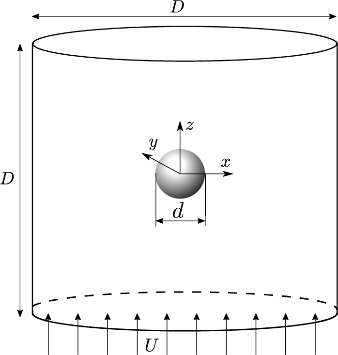
The problem of a sphere d moving in an infinite medium is modelled as a sphere fixed at the centre of a cylindrical tube with a uniform inflow U (Fig. 1). The tube has both diameter and length equal to D. The origin of the Cartesian reference frame is placed at the sphere centre with the z-axis aligned with flow direction.
Fig. 1.
Schematic representation of the problem.
The laminar, steady, isothermal and single-phase flow of an incompressible fluid is governed by the following continuity and momentum equations (in Cartesian coordinates):
The issue related to the infinite viscosity in equation Eq. (3) when
For Herschel–Bulkley fluids, the Papanastasiou regularisation would still produce an infinite viscosity for
Fig. 2.
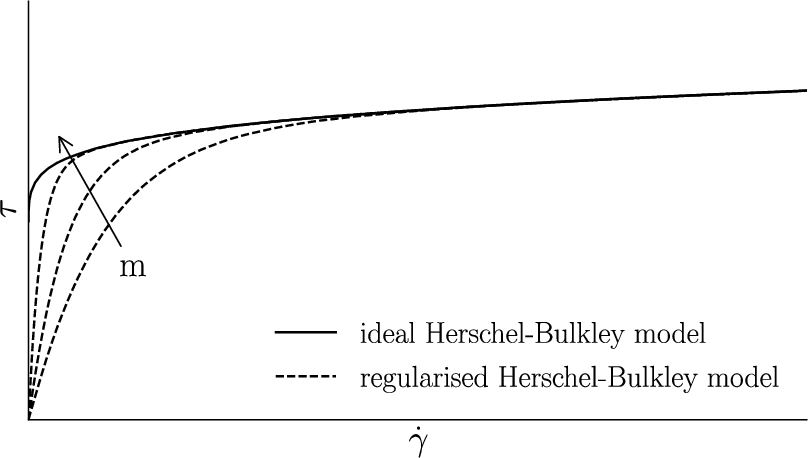
Effect of the regularisation parameter on the Herschel–Bulkley model.
3.Non-dimensional numbers and test cases
The Herschel–Bulkley flow around a sphere is characterised by two non-dimensional numbers: the generalised Reynolds number
The non-dimensional friction, pressure and drag coefficients are calculated respectively as
Furthermore, throughout the paper, the regularisation parameter m will be expressed in its non-dimensional form,
Numerical simulations are performed for all the combinations of
In addition, simulations are performed for creep flow (
For Bingham creep flow, the drag coefficient as defined in Eq. (8) becomes extremely large. The reason is that inertia is virtually zero for creep flows, hence
4.Numerical methods and setup
4.1.Flow solver
The CFD code used for the present work is ReFRESCO, in which the governing equations are discretised with a second-order finite-volume method for unstructured mesh with cell-centered co-located variables. Mass conservation is ensured with a pressure-correction equation based on a SIMPLE-like algorithm [26] and a pressure-weighted interpolation technique to avoid spurious oscillations [32]. The convective term in the momentum equation is linearised with the Picard method and discretised with a central difference scheme. Other features such as cavitation and turbulence models (the latter also for Herschel–Bulkley fluids [29]) are also implemented but not used in the present work. These and other numerical techniques are described in detail elsewhere (e.g. [19]).
4.2.Boundary conditions
The boundary conditions are set as follows. A uniform inflow
4.3.Domain size
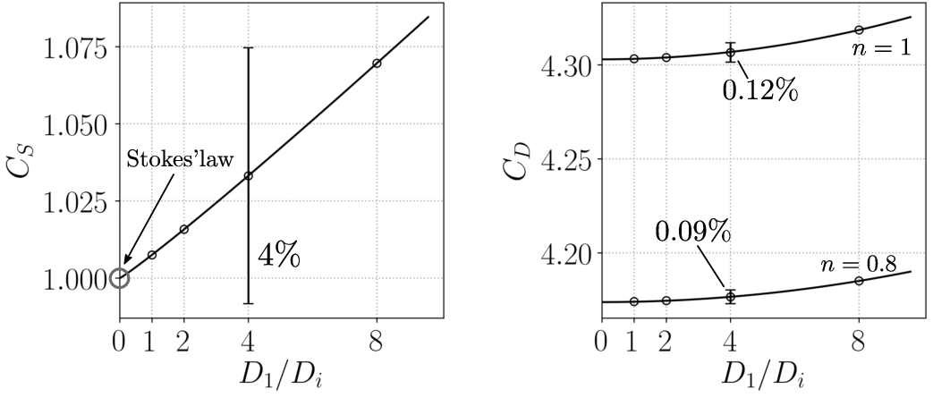
In order to mimic a sphere settling in an infinite domain, the outer cylindrical tube diameter must be sufficiently large compared to the sphere diameter. The influence of the tube-to-sphere diameter ratio,
The uncertainty in the solution due to the domain size has been estimated with the method of Eça and Hoekstra [17] by replacing the grid size with the tube diameter D. Since this method was designed to estimate the discretisation uncertainties, we have checked the validity of this procedure by performing additional calculations for Newtonian creep flow, whose exact solution for the unbounded domain yields
Fig. 3.
Convergence of the Stokes/drag coefficients with
The uncertainties were then estimated for all the test cases, and the two largest values obtained with
In conclusion, the maximum domain-size uncertainty for Newtonian and power-law fluid is about
4.4.Domain discretisation
The domain was discretised with two series of three-dimensional multi-block structured grids, with the layout as sketched in Fig. 4. Four geometrically similar grids were generated for each series in order to estimate the discretisation uncertainties. The number of grid cells and the size of the first cells away from the sphere surface are reported in Table 1. One series was generated for
Fig. 4.
Illustration of the coarsest grid of Series 1.
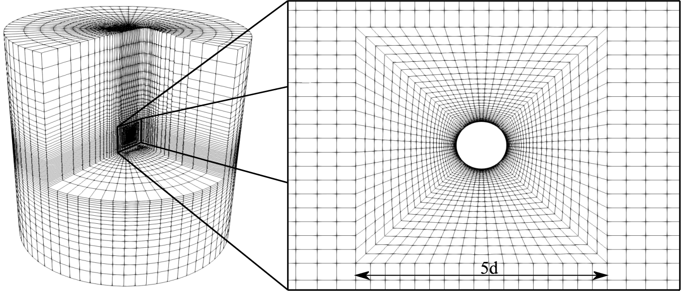
Table 1
Grid size ratio, number of cells
| i | Series 1 | Series 2 | ||||
| 4 | 2.59 | 129 064 | 0.00800 | 2.60 | 156 808 | 0.00200 |
| 3 | 1.90 | 324 070 | 0.00571 | 1.91 | 397 072 | 0.00143 |
| 2 | 1.38 | 857 600 | 0.00408 | 1.38 | 1 054 208 | 0.00102 |
| 1 | 1.00 | 2 238 368 | 0.00292 | 1.00 | 2 761 088 | 0.00073 |
Table 2
Discretisation uncertainties in percentage of the corresponding drag component for the pressure, frictional and total drag on the finest grid
| n | ||||||||||||||
| 10 | 1 | 0.03 | 0.12 | 0.09 | 0.88 | 0.17 | 0.25 | 0.40 | 0.38 | 0.36 | 2.299 | 0.61 | 0.25 | 0.36 |
| 10 | 0.8 | 0.02 | 0.11 | 0.08 | 0.34 | 0.10 | 0.57 | 0.34 | 0.94 | 0.38 | 8.047 | 0.56 | 0.39 | 0.43 |
| 10 | 0.6 | 0.02 | 0.09 | 0.05 | 0.31 | 0.18 | 0.26 | 0.33 | 3.34 | 0.76 | 59.59 | 0.28 | 0.21 | 0.20 |
| 100 | 1 | 0.10 | 0.05 | 0.07 | 0.28 | 0.10 | 0.17 | 0.32 | 0.30 | 0.30 | 340.7 | 0.49 | 0.12 | 0.42 |
| 100 | 0.8 | 0.18 | 0.11 | 0.15 | 0.33 | 0.09 | 0.24 | 0.30 | 0.88 | 0.39 | 497.5 | 0.24 | 0.15 | 0.22 |
| 100 | 0.6 | 0.38 | 0.23 | 0.31 | 0.19 | 0.17 | 0.25 | 0.66 | 3.26 | 0.69 | 544.6 | 0.24 | 0.21 | 0.23 |
The discretisation uncertainties on the force coefficients are given in Table 2 and they were estimated with the method of Eça and Hoekstra [17]. All the calculations were carried out using the regularisation parameters discussed in the following section. Except for the two cases with
4.5.Regularisation methods
The use of regularisation methods produces regularisation errors, which are defined as the difference between the solution obtained with the regularised and non-regularised rheological models. Large regularisation parameters are needed to minimise these errors, but this may lead to very slow or even stagnating convergence of the residuals in the iterative solver, as will be shown in Section 4.6.
For practical applications, however, low regularisation parameters may be acceptable since the rheology of many real fluids is better captured by regularised models (e.g. [15,18]). On the other hand, for the purpose of comparison with literature data it is important to minimise these errors, also to avoid possible cancellation of regularisation and discretisation errors that can cause a spurious agreement with literature data. Figure 5 shows an example in which
Fig. 5.
Grid convergence of the Stokes coefficient for
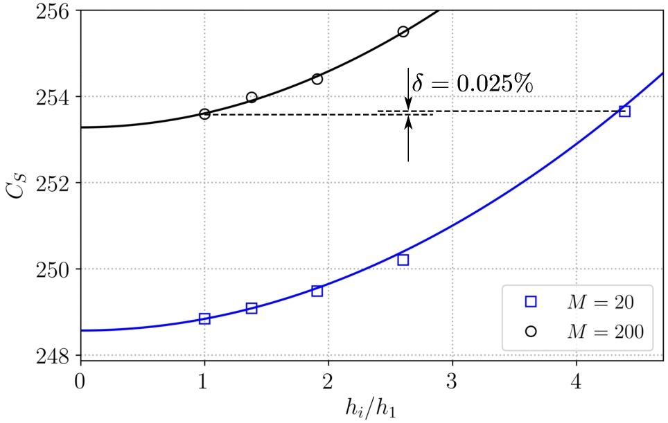
Fig. 6.
Convergence of the Stokes coefficient with
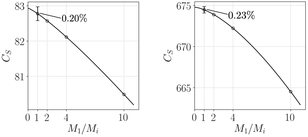
The choice of the proper regularisation parameter is found to be problem-dependent. With regard to the laminar flow around a sphere, previous numerical studies used very different values, both dimensional and non-dimensional. For instance, Blackery and Mitsoulis [8] used
For the current work, the regularisation parameter for each test case has been gradually increased until the regularisation uncertainty became less than 1%. The question, however, is how to estimate the regularisation uncertainty. Frigaard and Nouar [20] showed that, for typical Bingham shear flows, the Papanastasiou regularisation errors tend to zero with first order as
Table 3
Selected non-dimensional regularisation parameter
| Creep flow, | ||||||||||
| 10 | 100 | 10 | 100 | 2.299 | 8.047 | 59.59 | 197.5 | 340.7 | 544.6 | |
| 500 | 200 | 1000 | 200 | 2000 | 2000 | 200 | 200 | 200 | 200 | |
| 500 | 200 | 1000 | 200 | – | – | – | – | – | – | |
| 500 | 200 | 500 | 200 | – | – | – | – | – | – | |
Finally, we remark that the values reported in Table 3 may not be sufficient to accurately capture the so-called yielded surface, i.e. the locus of points where
4.6.Iterative convergence and viscosity interpolation scheme
As mentioned in the previous section, iterative convergence can become difficult when using large regularisation parameters. This issue seems rather common when using SIMPLE-like algorithms (see e.g. [40,41]). In this work, we found that the rate of convergence of the residuals is significantly influenced by the choice of the interpolation scheme for the viscosity.
Within the finite-volume method, the diffusive term in Eq. (1) requires the evaluation of the apparent viscosity, μ, at the cell faces. Since in ReFRESCO the computational node coincides with the cells’ centroid, the face value must be obtained by interpolation. Assuming for simplicity that a cell face e is halfway between two Cartesian grid cells P and E, the simplest second-order interpolation scheme to calculate
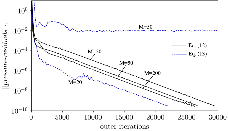
The two schemes have the same computational cost, thus, in principle, there is no reason to prefer one scheme to the other. Furthermore, when we performed a code verification exercise (not shown here) similar to that in [30], the two schemes exhibited the same accuracy and rate of convergence of the residuals. However, on the present problem, the first scheme (Eq. (12)) turned out to be more robust as it was possible to obtain a fully converged solution using relatively large regularisation parameters,11 as shown in Fig. 7. With the second scheme (Eq. (13)), on the other hand, the residuals were stagnating already with regularisation parameters that were one order of magnitude lower than those used to obtain a fully-converged solution with the first scheme. Therefore, an interpolation scheme that uses the cell centre values of the apparent viscosity was eventually adopted in ReFRESCO.
Fig. 7.
Effect of the two viscosity interpolation schemes on the iterative convergence of the pressure residuals. Test case:
For this work and with the setup described above, the iterative convergence criterion was set to
4.7.Total numerical uncertainty
The final numerical uncertainty in the computed drag coefficient was calculated assuming that all the uncertainty components are dependent on each other, hence
Table 4
Total numerical uncertainties,
| n | ||||||
| 10 | 1 | 0.21 | 0.63 | 0.55 | 2.299 | 0.55 |
| 10 | 0.8 | 0.16 | 0.85 | 0.50 | 8.047 | 0.53 |
| 10 | 0.6 | 0.10 | 0.45 | 0.83 | 59.59 | 0.44 |
| 100 | 1 | 0.19 | 0.94 | 0.55 | 340.7 | 0.52 |
| 100 | 0.8 | 0.24 | 0.85 | 0.56 | 497.5 | 0.30 |
| 100 | 0.6 | 0.38 | 1.02 | 0.80 | 544.6 | 0.29 |
5.Results and discussion
5.1.Flow field
Some features of the computed flow field are now discussed. More detailed descriptions have been already discussed by other authors [7,22,34,35], thus they will not be completely repeated here. The contours of the velocity, shear rate and viscosity for
Fig. 8.
Velocity contour and streamlines. The flow is from bottom to top.
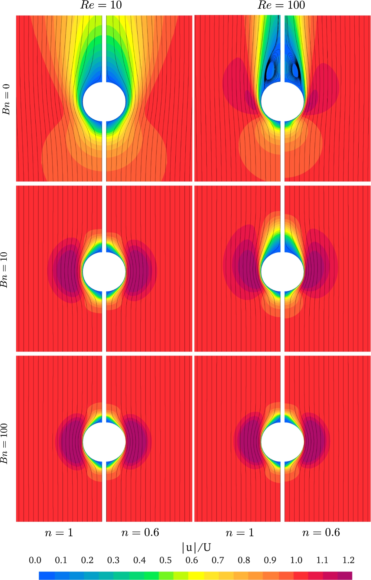
Fig. 9.
Contour plot of the shear rate
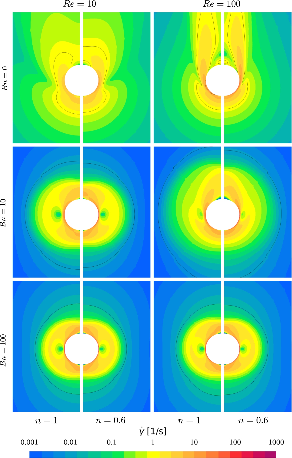
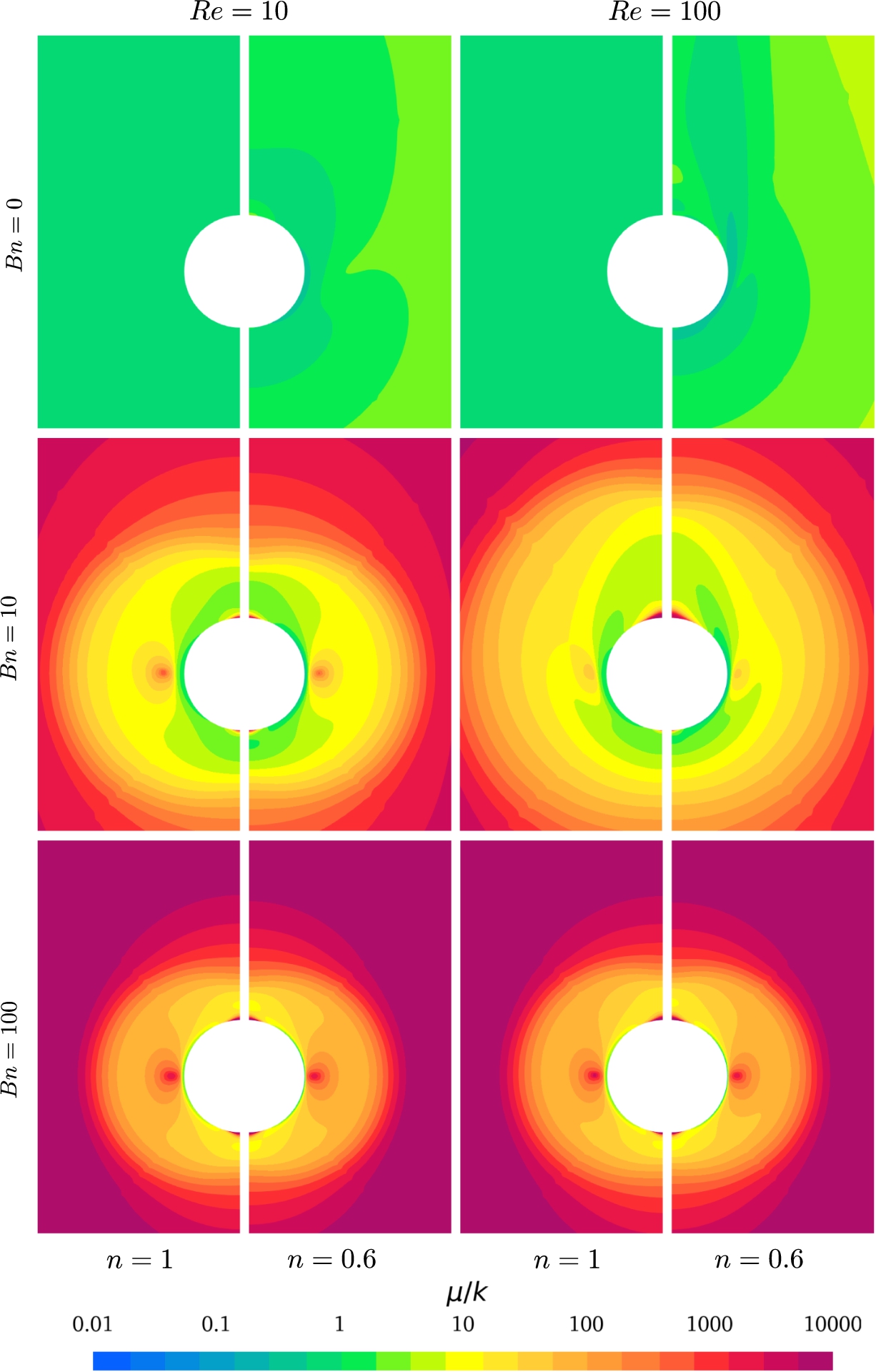
Fig. 10.
Contour plot of
For Newtonian and power-law fluids (
For yield stress fluids (
When
As
Furthermore, for yield stress fluids, the velocity in the equatorial plane exhibits a local maximum, which leads to a local viscosity maximum22 (Fig. 10), as also observed in [22,34]. Such steep variation of viscosity over a relative short distance was a major cause for the difficult iterative convergence. We found in fact that the largest residuals were always near the local viscosity maximum.
For ideal (i.e. non-regularised) Bingham and Herschel–Bulkley fluids, the fluid region far from the sphere would have an infinite viscosity and zero shear rate. The effect of the regularisation is evident in Figs 9 and 10: the shear rate is very low (but not zero) and the viscosity is very large (but not infinite).
Fig. 11.
Axial velocity profiles for Bingham fluids (

Finally, the velocity profiles for Bingham fluids at
In conclusion, the flow field is qualitatively in line with previous studies from the literature, and it quantitatively agrees with the results of Gavrilov et al. and Nirmalkar et al.
5.2.Drag coefficients and comparison with literature
The drag coefficient is often the only quantity of interest in many engineering applications. It is therefore a meaningful quantity to assess whether the present code can reproduce the results from the literature.
Table 5
Pressure, frictional and total drag coefficients for all the considered test cases
| n | ||||||||||||||
| 10 | 1 | 1.528 | 2.781 | 4.308 | 25.10 | 18.30 | 43.39 | 223.1 | 97.62 | 320.8 | 2.299 | 3.071 | 3.325 | 6.395 |
| 10 | 0.8 | 1.641 | 2.537 | 4.178 | 25.00 | 15.22 | 40.22 | 222.9 | 86.25 | 309.2 | 8.047 | 8.599 | 6.668 | 15.27 |
| 10 | 0.6 | 1.799 | 2.222 | 4.021 | 24.86 | 12.45 | 37.31 | 222.6 | 77.99 | 300.6 | 59.59 | 55.93 | 26.85 | 82.78 |
| 100 | 1 | 0.512 | 0.577 | 1.089 | 2.789 | 1.915 | 4.704 | 22.41 | 9.775 | 32.18 | 340.7 | 181.9 | 71.71 | 253.6 |
| 100 | 0.8 | 0.494 | 0.446 | 0.940 | 2.764 | 1.570 | 4.334 | 22.39 | 8.632 | 31.02 | 497.5 | 312.7 | 115.3 | 428.0 |
| 100 | 0.6 | 0.471 | 0.320 | 0.790 | 2.722 | 1.261 | 3.983 | 22.36 | 7.802 | 30.16 | 544.6 | 499.0 | 175.5 | 674.5 |
The drag coefficients and its components are reported in Table 5. The ratio
Table 6
Drag coefficient,
| Data from | |||||||
| present work | 4.308 | 4.178 | 4.021 | 1.089 | 0.940 | 0.790 | |
| Dhole [14] | 4.281 | 4.086 | 3.769 | 1.062 | 0.921 | 0.759 | |
| Tripathi [43] | 4.31 | 4.17 | 3.76 | 1.02 | 0.920 | 0.780 | |
| Gavrilov [22] | 4.334 | 4.167 | 3.969 | 1.095 | 0.941 | 0.787 | |
| present work | 43.39 | 40.22 | 37.31 | 4.704 | 4.334 | 3.983 | |
| Gavrilov [22] | 42.15 | 38.90 | 35.91 | 4.587 | 4.217 | 3.880 | |
| Nirmalkar [34,35] | 43.63 | 40.40 | 37.43 | 4.743 | 4.363 | 4.015 | |
| present work | 320.8 | 309.2 | 300.6 | 32.18 | 31.02 | 30.16 | |
| Gavrilov [22] | 307.9 | 295.4 | 284.7 | 30.95 | 29.69 | 28.61 | |
A direct comparison of
Table 7
Stokes coefficients,
| Data from | ||||||
| 8.047 | 59.59 | 197.5 | 340.7 | 544.6 | ||
| present work | 6.395 | 15.27 | 82.78 | 253.6 | 428.0 | 674.5 |
| Beris [7] | 6.39 | 15.24 | 82.77 | 252.2 | 426.9 | 669.7 |
| Liu [28] | 6.38 | 15.21 | 82.67 | 253.6 | 426.0 | 671.9 |
| Nirmalkar [34] | – | 15.25 | 82.83 | – | 427.5 | 673.5 |
E and
Fig. 12.
Comparison error (± validation uncertainty) for the drag coefficient in percentage of our data for
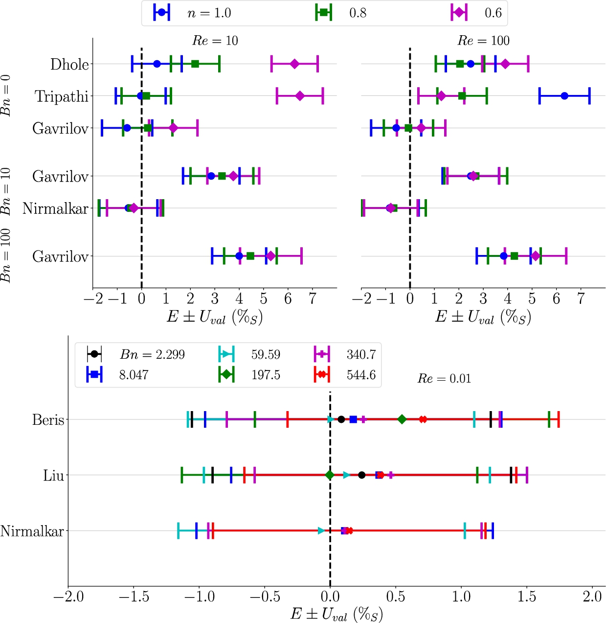
The comparison errors and the validation uncertainties are plotted in Fig. 12, from which the following observations are made:
For power-law fluids (
For Bingham and Herschel–Bulkley fluids (
The best agreement with literature data is achieved for Bingham creep flow (
Our results tend to be on the over-predicting side, i.e. E leans towards the right side of Fig. 12. We observed that
6.Conclusions
We have tested the viscous-flow solver ReFRESCO on the laminar non-Newtonian flow around a sphere as a stepping stone towards more practical maritime applications.
Some difficulties were encountered when using large regularisation parameters, which led to stagnating residuals and thus large iterative errors. A determining factor turned out to be the choice of the viscosity interpolation scheme. Although obtaining a fully converged solutions remained challenging, the improved iterative convergence provided a significant reduction of the iterative and regularisation errors. This allowed a more compelling comparison with literature.
The flow field around the sphere exhibited the expected behaviour for the considered test cases and it is both qualitatively and quantitatively consistent with previous numerical studies. The maximum difference in drag coefficient between the calculated values and the values from the literature reached 7% (i.e. outside the validation uncertainty range) for power-law fluids, whereas it was insignificant for Bingham creep flow. Overall, the agreement with previous studies is good, with discrepancies that are, in most cases, close or within the validation uncertainties.
Combining the evidence of our previous code verification exercises [30,31] and the results of this work, it is concluded that the power-law, Bingham and Herschel–Bulkley models are implemented correctly and that the code is capable of reproducing literature data with good accuracy despite the high non-linearity introduced by the non-Newtonian viscosity. This provides confidence to employ ReFRESCO for more complex applications such as a ship sailing through fluid mud. Finally, present data can be used for future verifications and to derive new correlations for the drag coefficient.
Credit author statement
Stefano Lovato: Conceptualization, Software, Investigation, Validation, Visualization, Writing – Original Draft. Serge Toxopeus: Software, Validation, Supervision, Writing - Review & Editing. Just Settels: Validation, Supervision, Writing – Review & Editing. Geert Keetels: Supervision, Funding acquisition, Writing – Review & Editing.
Conflict of interest
Serge Toxopeus is an Editorial Board Member of this journal, but was not involved in the peer-review process nor had access to any information regarding its peer-review.
Notes
1 Sufficiently large, at least, to keep the regularisation uncertainty below 1%.
2 Note that, in three dimensions, this local maximum is actually a circle around the sphere.
Acknowledgement
This research is funded by the Division for Earth and Life Sciences (ALW) with financial aid from the Netherlands Organization for Scientific Research (NWO) with Grant No.ALWTW.2016.029. Calculations were performed on the Reynolds (TU Delft) and Marclus4 (MARIN) clusters. The research support from MARIN is partly funded by the Dutch Ministry of Economic Affairs. The authors wish to thank Andrey Gavrilov and Neelkanth Nirmalkar for kindly providing their data. This study was carried out within the framework of the MUDNET academic network: https://www.tudelft.nl/mudnet/.
References
[1] | R.W. Ansley and T.N. Smith, Motion of spherical particles in a Bingham plastic, AIChE Journal 13: (6) ((1967) ), 1193–1196. doi:10.1002/aic.690130629. |
[2] | A.S. Arabi and R.S. Sanders, Particle terminal settling velocities in non-Newtonian viscoplastic fluids, Canadian Journal of Chemical Engineering 94: (6) ((2016) ), 1092–1101. doi:10.1002/cjce.22496. |
[3] | ASME PTC Committee, Standard for Verification and Validation in Computational Fluid Dynamics and Heat Transfer: ASME V&V 20, The American Society of Mechanical Engineers (ASME) (2009). |
[4] | D.D. Atapattu, R.P. Chhabra and P.H.T. Uhlherr, Wall effect for spheres falling at small Reynolds number in a viscoplastic medium, Journal of Non-Newtonian Fluid Mechanics 38: (1) ((1990) ), 31–42. doi:10.1016/0377-0257(90)85031-S. |
[5] | D.D. Atapattu, R.P. Chhabra and P.H.T. Uhlherr, Creeping sphere motion in Herschel–Bulkley fluids: flow field and drag, Journal of Non-Newtonian Fluid Mechanics 59: (2–3) ((1995) ), 245–265. doi:10.1016/0377-0257(95)01373-4. |
[6] | M. Beaulne and E. Mitsoulis, Creeping motion of a sphere in tubes filled with Herschel–Bulkley fluids, Journal of Non-Newtonian Fluid Mechanics 72: (1) ((1997) ), 55–71. doi:10.1016/S0377-0257(97)00024-4. |
[7] | A.N. Beris, J.A. Tsamopoulos, R.C. Armstrong and R.A. Brown, Creeping motion of a sphere through a Bingham plastic, Journal of Fluid Mechanics 158: ((1985) ), 219–244. doi:10.1017/S0022112085002622. |
[8] | J. Blackery and E. Mitsoulis, Creeping motion of a sphere in tubes filled with a Bingham plastic material, Journal of Non-Newtonian Fluid Mechanics 70: (1–2) ((1997) ), 59–77. doi:10.1016/S0377-0257(96)01536-4. |
[9] | B.J. Briscoe, M. Glaese, P.F. Luckham and S. Ren, The falling of spheres through Bingham fluids, Colloids and Surfaces 65: (1) ((1992) ), 69–75. doi:10.1016/0166-6622(92)80176-3. |
[10] | G.R. Burgos, A.N. Alexandrou and V. Entov, On the determination of yield surfaces in Herschel–Bulkley fluids, Journal of Rheology 43: (3) ((1999) ), 463–483. doi:10.1122/1.550992. |
[11] | R.P. Chhabra, Bubbles, Drops, and Particles in Non-Newtonian Fluids, CRC Press, (2006) . doi:10.1201/9781420015386. |
[12] | P. Coussot and J.M. Piau, On the behavior of fine mud suspensions, Rheologica Acta 33: (3) ((1994) ), 175–184. doi:10.1007/BF00437302. |
[13] | G. Dazhi and R.I. Tanner, The drag on a sphere in a power-law fluid, Journal of Non-Newtonian Fluid Mechanics 17: (1) ((1985) ), 1–12. doi:10.1016/0377-0257(85)80001-X. |
[14] | S.D. Dhole, R.P. Chhabra and V. Eswaran, Flow of power-law fluids past a sphere at intermediate Reynolds numbers, Industrial & Engineering Chemistry Research 45: (13) ((2006) ), 4773–4781. doi:10.1021/ie0512744. |
[15] | N.Q. Dzuy and D.V. Boger, Direct yield stress measurement with the Vane method, Journal of Rheology 29: (3) ((1985) ), 335–347. doi:10.1122/1.549794. |
[16] | L. Eça and M. Hoekstra, Evaluation of numerical error estimation based on grid refinement studies with the method of the manufactured solutions, Computers & Fluids 38: (8) ((2009) ), 1580–1591. doi:10.1016/j.compfluid.2009.01.003. |
[17] | L. Eça and M. Hoekstra, A procedure for the estimation of the numerical uncertainty of CFD calculations based on grid refinement studies, Journal of Computational Physics 262: ((2014) ), 104–130. doi:10.1016/j.jcp.2014.01.006. |
[18] | K.R.J. Ellwood, G.C. Georgiou, T.C. Papanastasiou and J.O. Wilkes, Laminar jets of Bingham-plastic liquids, Journal of Rheology 34: (6) ((1990) ), 787–812. doi:10.1122/1.550144. |
[19] | J.H. Ferziger and M. Perić, Computational Methods for Fluid Dynamics, Springer, Berlin Heidelberg, Berlin, Heidelberg, (1996) . doi:10.1007/978-3-642-97651-3. |
[20] | I.A.A. Frigaard and C. Nouar, On the usage of viscosity regularisation methods for visco-plastic fluid flow computation, Journal of Non-Newtonian Fluid Mechanics 127: (1) ((2005) ), 1–26. doi:10.1016/j.jnnfm.2005.01.003. |
[21] | Z. Gao, H. Yang and M. Xie, Computation of flow around Wigley hull in shallow water with muddy seabed, Journal of Coastal Research 73: ((2015) ), 490–495. doi:10.2112/SI73-086.1. |
[22] | A.A. Gavrilov, K.A. Finnikov and E.V. Podryabinkin, Modeling of steady Herschel–Bulkley fluid flow over a sphere, Journal of Engineering Thermophysics 26: (2) ((2017) ), 197–215. doi:10.1134/S1810232817020060. |
[23] | D.I. Graham and T.E.R. Jones, Settling and transport of spherical particles in power-law fluids at finite Reynolds number, Journal of Non-Newtonian Fluid Mechanics 54: (C) ((1994) ), 465–488. doi:10.1016/0377-0257(94)80037-5. |
[24] | F. Irgens, Rheology and Non-Newtonian Fluids, Springer International Publishing, Cham, (2014) , pp. 1–190. doi:10.1007/978-3-319-01053-3. |
[25] | S. Kaidi, E. Lefrançois and H. Smaoui, Numerical modelling of the muddy layer effect on ship’s resistance and squat, Ocean Engineering 199: ((2020) ), 106939. doi:10.1016/j.oceaneng.2020.106939. |
[26] | C.M. Klaij and C. Vuik, SIMPLE-type preconditioners for cell-centered, colocated finite volume discretization of incompressible Reynolds-averaged Navier–Stokes equations, International Journal for Numerical Methods in Fluids 71: (7) ((2013) ), 830–849. doi:10.1002/fld.3686. |
[27] | K. Koziol and P. Glowacki, Determination of the free settling parameters of spherical particles in power law fluids, Chemical Engineering and Processing: Process Intensification 24: (4) ((1988) ), 183–188. doi:10.1016/0255-2701(88)85001-3. |
[28] | B.T. Liu, S.J. Muller and M.M. Denn, Convergence of a regularization method for creeping flow of a Bingham material about a rigid sphere, Journal of Non-Newtonian Fluid Mechanics 102: (2) ((2002) ), 179–191. doi:10.1016/S0377-0257(01)00177-X. |
[29] | S. Lovato, G.H. Keetels, S.L. Toxopeus and J.W. Settels, An Eddy-viscosity model for turbulent flows of Herschel–Bulkley fluids, Journal of Non-Newtonian Fluid Mechanics 301: ((2022) ), 104729. doi:10.1016/j.jnnfm.2021.104729. |
[30] | S. Lovato, S.L. Toxopeus, J.W. Settels, G.H. Keetels and G. Vaz, Code verification of non-Newtonian fluid solvers for single- and two-phase laminar flows, Journal of Verification, Validation and Uncertainty Quantification 6: (2) ((2021) ). doi:10.1115/1.4050131. |
[31] | S. Lovato, G. Vaz, S.L. Toxopeus, G.H. Keetels and J.W. Settels, Code verification exercise for 2D Poiseuille flow with non-Newtonian fluid, in: Numerical Towing Tank Symposium (NuTTS), (2018) . |
[32] | T.F. Miller and F.W. Schmidt, Use of a pressure-weighted interpolation method for the solution of the incompressible Navier–Stokes equations on a nonstaggered grid system, Numerical Heat Transfer 14: (2) ((1988) ), 213–233. doi:10.1080/10407788808913641. |
[33] | K.A. Missirlis, D. Assimacopoulos, E. Mitsoulis and R.P. Chhabra, Wall effects for motion of spheres in power-law fluids, Journal of Non-Newtonian Fluid Mechanics 96: (3) ((2001) ), 459–471. doi:10.1016/S0377-0257(00)00189-0. |
[34] | N. Nirmalkar, R.P. Chhabra and R.J. Poole, Numerical predictions of momentum and heat transfer characteristics from a heated sphere in yield-stress fluids, Industrial & Engineering Chemistry Research 52: (20) ((2013) ), 6848–6861. doi:10.1021/ie400703t. |
[35] | N. Nirmalkar, R.P. Chhabra and R.J. Poole, Effect of shear-thinning behavior on heat transfer from a heated sphere in yield-stress fluids, Industrial & Engineering Chemistry Research 52: (37) ((2013) ), 13490–13504. doi:10.1021/ie402109k. |
[36] | T.C. Papanastasiou, Flows of materials with yield, Journal of Rheology 31: (5) ((1987) ), 385–404. doi:10.1122/1.549926. |
[37] | P. Saramito and A. Wachs, Progress in numerical simulation of yield stress fluid flows, Rheologica Acta 56: (3) ((2017) ), 211–230. doi:10.1007/s00397-016-0985-9. |
[38] | P.R. Souza Mendes and E.S.S. Dutra, Viscosity function for yield-stress liquids, Applied Rheology 14: (6) ((2004) ), 296–302. doi:10.1515/arh-2004-0016. |
[39] | G.G. Stokes, On the effect of the internal friction of fluids on the motion of pendulums, in: Mathematical and Physical Papers, Cambridge University Press, Cambridge, (2010) , pp. 1–10. doi:10.1017/CBO9780511702266.002. |
[40] | A. Syrakos, G.C. Georgiou and A.N. Alexandrou, Solution of the square lid-driven cavity flow of a Bingham plastic using the finite volume method, Journal of Non-Newtonian Fluid Mechanics 195: ((2013) ), 19–31. doi:10.1016/j.jnnfm.2012.12.008. |
[41] | A. Syrakos, G.C. Georgiou and A.N. Alexandrou, Performance of the finite volume method in solving regularised Bingham flows: Inertia effects in the lid-driven cavity flow, Journal of Non-Newtonian Fluid Mechanics 208–209: ((2014) ), 88–107. doi:10.1016/j.jnnfm.2014.03.004. |
[42] | H. Tabuteau, P. Coussot and J.R. de Bruyn, Drag force on a sphere in steady motion through a yield-stress fluid, Journal of Rheology 51: (1) ((2007) ), 125–137. doi:10.1122/1.2401614. |
[43] | A. Tripathi, R.P. Chhabra and T. Sundararajan, Power law fluid flow over spheroidal particles, Industrial & Engineering Chemistry Research 33: (2) ((1994) ), 403–410. doi:10.1021/ie00026a035. |
[44] | L. Valentik and R.L. Whitmore, The terminal velocity of spheres in Bingham plastics, British Journal of Applied Physics 16: (8) ((1965) ), 1197–1203. doi:10.1088/0508-3443/16/8/320. |
[45] | G. Vaz, F. Jaouen and M. Hoekstra, Free-surface viscous flow computations: Validation of URANS code FRESCO, in: Proceedings of OMAE2009, Honolulu, Hawaii, USA, (2009) , pp. 425–437. doi:10.1115/OMAE2009-79398. |
[46] | R.W. Wurpts, 15 years experience with fluid mud: Definition of the nautical bottom with rheological parameters, Terra et Aqua (2005). |


