A technique for efficient computation of steady yaw manoeuvres using CFD

1.Introduction

To numerically predict ship manoeuvres using Computational Fluid Dynamics (CFD), different approaches can be used. Directly simulating the manoeuvre with unsteady CFD, including the movement of appendages and sometimes even the propeller, is a straightforward method which can produce good results as shown by Carrica et al. [5] or during recent SIMMAN workshops [27]. However, such applications can be complex and time-consuming and they cannot be applied for real-time manoeuvring studies. Alternatively, the manoeuvres can be predicted using simulation software which use mathematical manoeuvring models based on CFD results, see e.g. Cura Hochbaum et al. [7] or Toxopeus and Lee [36]. These models describe the forces and moments acting on the ship as a function of the manoeuvring parameters, such as for example speed, drift angle and yaw rate. The hydrodynamic loads acting on a ship sailing at a constant speed can nowadays be reliably computed using CFD as shown for example during the Workshops on CFD in Ship Hydrodynamics [17,18] or NATO studies [21,22].

To obtain the coefficients in the mathematical manoeuvring model, series of (captive) CFD simulations need to be conducted. For a three degrees-of-freedom (DoF) model of the bare hull forces, these series can consist of static drift manoeuvres [3,35], static rotational yaw motion combined with a drift angle [32,33] and/or dynamic manoeuvres [4,8,12].

When free surface effects are expected to play a minor role (generally for Froude numbers below 0.13) and when added mass coefficients are available from other sources (e.g. from potential flow calculations) it can be sufficient to restrict the CFD computations to steady simulations for static motions only, which is attractive due to low CPU costs and straightforward analysis of the results. This has also been observed by for example Oldfield et al. [24].

Static drift manoeuvres consist of simulations in which the vessel encounters a uniform inflow at a certain drift or inflow angle. During static rotational yaw motion the ship rotates with a constant ship-fixed velocity with a given turn radius, often combined with a drift angle. Traditionally, ample attention has been paid to drift manoeuvres due to their simplicity and the large amount of available validation data. Rotational motion has received much less attention [32], since specialised facilities are required to generate validation data and the numerical setup for static rotation is more complex than for static drift. This is also reflected in the much lower number of cases and submissions for yaw motions than for static drift motions during the SIMMAN 2014 workshop [28]. At MARIN, however, computations for yaw motions have been done extensively, for example in the EU project NOVIMAR for conditions with different water depths [34], in order to obtain mathematical manoeuvring models. The experience obtained with performing large sets of CFD computations has led to an improved CFD approach.

In this paper, options found in literature of steady rotational motion simulations with CFD will be discussed. First, the common approach using a non-inertial reference frame is presented in Section 2, together with difficulties often encountered with such an approach, i.e. how to deal with the grid, the numerical setup and the wake of the vessel. Subsequently, an example of such an approach for shallow water conditions will be given in Section 3, further highlighting the difficulties. Finally, this paper will present a modified approach, leading to an improved work flow for captive manoeuvring computations for mathematical manoeuvring models, which will be more efficient in preprocessing (due to the use of a single grid for all computations) and computing time (due to improved iterative convergence) as well as more reliable due to the suppression of the vessel’s wake at high yaw rates.

The objective of this paper is to provide guidelines on how to reliably conduct CFD computations for static yaw motion, using a strategy that is both accurate and efficient.

Post-processing of the CFD involves fitting of the resulting hydrodynamic loads from which the manoeuvring coefficients are ultimately derived. The process of extracting the coefficients from the computed data is highly dependent on the underlying mathematical manoeuvring model (compare for instance Toxopeus [31] with Ferrari and Quadvlieg [10]) and therefore lies beyond the scope of this study.

2.Common approach for the simulation of rotational motion using CFD

Several examples of computations of captive yaw manoeuvres can be found in literature, such as e.g. Ohmori [23], Alessandrini and Delhommeau [1] or Cura Hochbaum [6]. All these methods use a non-inertial reference system to model the flow around the ship. In this way, a stationary ship-fixed coordinate system is adopted and the flow moves under the influence of body forces through the domain. With such an approach, it is possible to perform steady CFD computations which make it cost effective compared to unsteady computations. Also other approaches are used, such as a hybrid reference frame method of Wu et al. [39], but those do not seem to be widely adopted in the CFD community yet.

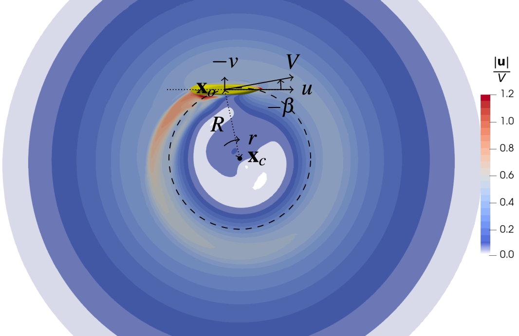
Fig. 1.

Velocity contours resulting from a steady computation of a rotational manoeuvre with drift in shallow water. Notice that the upstream flow velocity in front of the bow is far from zero.

The relation between the ship length between perpendiculars Lpp, turn radius R and non-dimensional yaw rate r′ is r′=Lpp/R. When considering a range of rotation rates, the centre of rotation moves closer towards the ship for increasing yaw rates. At a high enough yaw rate, the centre of rotation is located in the CFD domain and the possibility exists that the wake of the ship will convect through the domain. Ultimately, the ship will sail in its own wake as shown in Fig. 1 and the loads acting on the ship will be affected. With a lateral domain boundary placed 3Lpp from the ship, it can be expected that the wake will influence the results when the turning radius is about 2Lpp or less, i.e. for yaw rates exceeding r′=Lpp/(2Lpp)=0.5. In shallow water conditions, however, larger domain sizes are required [13,29] to avoid any influence of the side boundaries on the results and therefore the wake will influence the loads already at lower yaw rates. It is therefore important to mitigate the effect of the wake on the forces on the ship when using steady CFD for rotational motion.

Another problem with the centre of rotation being located inside the domain is the possibility of difficult convergence of the flow near the centre of rotation, and the difficulty in choosing the boundary condition at the boundary near the centre of rotation: part of this boundary will be inflow, while the other part will be an outflow, see for instance Fig. 3 in the ITTC guideline on the use of RANS tools for manoeuvring predictions [15]. Sometimes, the transition from inflow to outflow between neighbour faces on the boundary can pose convergence issues. This is also the reason that several publications show grid setups where the grid has a cut out and a split of the farfield boundary close to the centre of rotation.

Fig. 2.

Grid setup commonly used for static yaw rate computations (reproduced from Franceschi et al. [11]).

In literature, several approaches for the grid design can be found, such as designing the grid specifically for the given manoeuvring condition as done by Zhang et al. [14,40], Franceschi et al. [11] or Park et al. [26]. An example is included in Fig. 2, reproduced from [11]. Such an approach means that every computation needs a separate and dedicated grid. Furthermore, for high rotation rates, the boundary near the rotation centre is located close to the ship and can therefore influence the flow near the ship, especially in shallow water. To avoid spending time on grid generation and remove the influence of different grids and the proximity of boundary conditions on the results, a more efficient approach, using a single grid for all computations, is desired.

A time-dependent simulation, in which for example a moving mesh technique or a relative formulation of the flow equations is used to make the vessel traverse a segment of the turning circle, is a more accurate approximation of the desired manoeuvring condition. The manoeuvre commences in undisturbed water and continues up to a certain angle of rotation, but surely before encountering any remnants of its wake. Start-up effects need to be dealt with, but ultimately the hydrodynamic loads should stabilise when a steady state condition is obtained. The time integration process however increases the complexity and most noticeably the calculation time of a complete simulation. Furthermore, attempts in shallow water show that a steady state condition of the loads is not always fully reached before encountering the wake even after a substantial part of the turning circle has been traversed. In that case, one might have to resort to oscillatory yaw computations which have the disadvantage of a possible dependency of the hydrodynamic loads on the oscillation frequency, in addition to more complex post-processing to extract the hydrodynamic coefficients. Thus, although the closest approximation of the desired configuration, unsteady computations unfortunately do not always guarantee usable results in the process of constructing a mathematical manoeuvring model.

In the following section, an illustration of the problem in shallow water conditions will be given.

3.Illustrative case in shallow water conditions

To visualise the problem at hand a set of simulations is performed of static combined yaw-drift manoeuvres in shallow water conditions. Shallow water conditions are selected for two reasons. The additional confinement due to the bottom of the domain in shallow water generally causes higher loads on the vessel and fluctuations in velocity and pressure to decay at a lower rate than they normally would in deep water. This makes a simulation case in shallow water therefore a good demonstration of an extreme situation. A second argument is that, as discussed in the previous section, unsteady simulations that cover a partial turning circle are currently serving as a reference result assuming they converge to a steady state condition at some point. The convergence is generally no problem in deep water, but attempts in shallow water conditions have shown that this is not always trivial. Without a converged unsteady result, and with the knowledge that the traditional steady approach is definitely inaccurate, one is left with no solution at all. A shallow water simulation is therefore a good case to demonstrate the difficulties in obtaining the solution for a given manoeuvring condition. The approach taken in this example is representative of approaches used in literature and is therefore in this article referred to as the default approach.

3.1.Setup of the manoeuvring condition

Fig. 3.

Positive orientation of the ship motions, velocities and relevant loads.

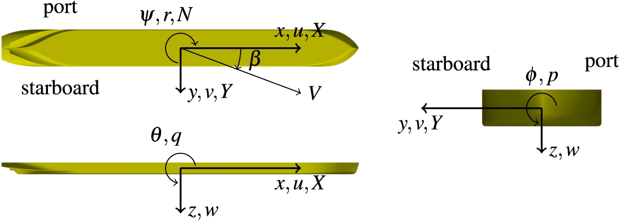
A ship-fixed right-handed coordinate system commonly used for manoeuvring studies is adopted, with x directed forward, y to starboard and z vertically down and the origin xo at the intersection of midship, water plane and the longitudinal plane of symmetry, see Fig. 3.

The case of a rotational manoeuvre around a fixed point xc with a fixed radius R=‖xc−xo‖ and constant forward sailing velocity V and yaw rate r=V/R is considered, as shown in Fig. 1. The yaw rate is made non-dimensional using the length between perpendiculars Lpp and the sailing velocity V: r′=r·Lpp/V⇒r′=Lpp/R.

The coordinates of the centre xc of the turning circle in the x−y plane for given values of Lpp, r′ and drift angle β=arctanv/u are given by:

(1)xcyc=xoyo+Lppr′−sinβcosβ,r′≠0.

A series of simulations is performed with non-dimensional yaw rates r′ varying from 0.1 to 0.7. A drift angle β is applied such that r·β<0 to assure a realistic configuration in which the bow points into the turn. Additionally, this ensures a sizeable magnitude of the transverse force compared to a zero drift configuration where Y is often small and inconsistent in sign. A complete set of steady simulations adopting a non-inertial reference frame as discussed in Section 2 is performed. Additionally, unsteady simulations using a moving grid approach are conducted for subsequent comparison of the forces and moments. The hydrodynamic forces X, Y and the yaw moment N as defined in Fig. 3 are made non-dimensional using the constant sailing velocity V, the ship length Lpp, its draught T and the water density ρ in the following way:

(2)X′=X12ρV2LppT,Y′=Y12ρV2LppT,N′=N12ρV2Lpp2T.

3.3.Computational domain and mesh

The ship is centrally placed in a rectangular domain of dimensions 10Lpp×10Lpp×0.038Lpp, as shown in Fig. 4(a), with a depth-to-draught ratio h/T equal to 1.2. From Equation (1) it subsequently follows that for r′=Lpp/R>0.4 the rotation centre xc is halfway between the ship and the boundary and therefore the circular path of the ship lies completely within the computational domain. For lower yaw rates, the path is interrupted by the starboard domain wall.

Fig. 4.

Computational domain and mesh used in the shallow water simulations.

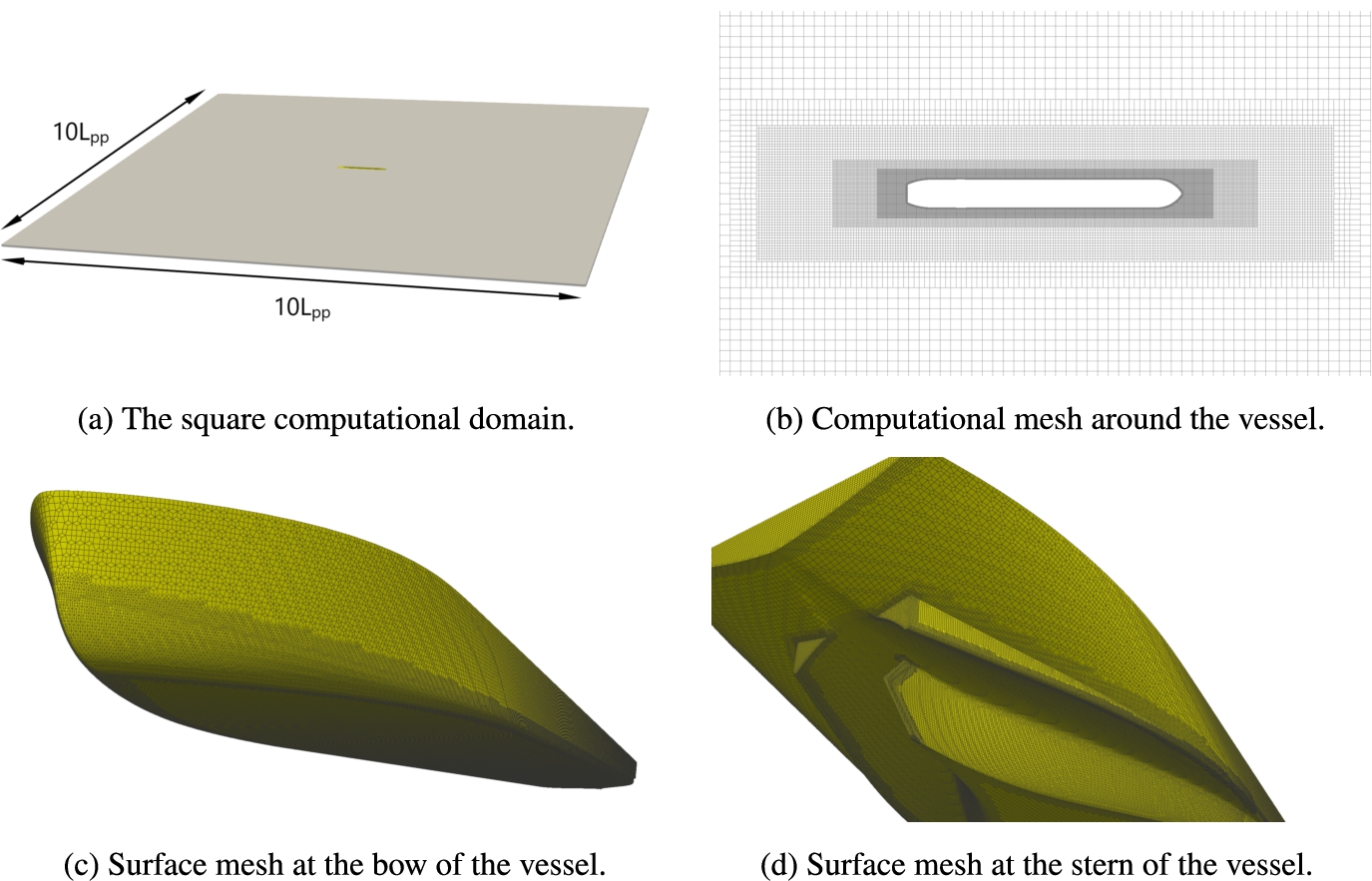
An unstructured hexahedral mesh is constructed using Hexpress, a commercial grid generator. Hanging nodes are present in the mesh to allow local grid refinements, and these are placed with progressive density around the ship as shown in Fig. 4(b). Anisotropic refinement in the direction normal to the hull is applied to fully resolve the boundary layer, keeping the y+-value below one. Refinement is also placed on the domain bottom around the contours of the ship to capture any possible boundary layer interaction below the hull. An impression of the surface mesh on the vessel is shown in Fig. 4(c) for the bow and in Fig. 4(d) for the stern. The mesh contains 11.1 million volume cells, and the vessel is represented by 261 thousand faces.

Because of the low Froude number, the undisturbed water surface is modelled as a symmetry plane in the simulation. All vertical boundaries are modelled as inflow boundaries with a prescribed Dirichlet condition for the velocity, and the bottom and ship hull are considered no-slip boundaries. The ship itself is held captive without any change in trim or sinkage during the simulation.

3.6.Rotation simulation results with the default method

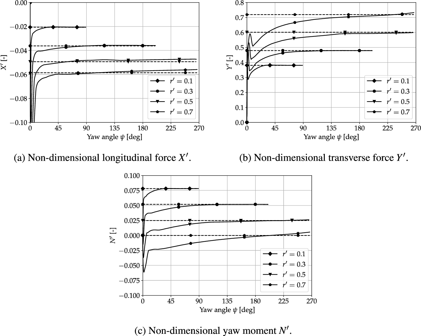
The hydrodynamic loads resulting from the sets of default steady and unsteady simulations are shown in Fig. 5. The time dependency of the unsteady results is converted into the angular displacement from rest. The steady results are plotted as horizontal lines for better comparison (as they are independent of the angle). When an unsteady result converges to the same value as its associated steady result, the steady approach can be considered a reliable technique to obtain the hydrodynamic loads, at lower computational cost.

Fig. 5.

Hydrodynamic loads computed using steady (dashed lines) and unsteady (solid lines) simulations in shallow water conditions for different turning rates.

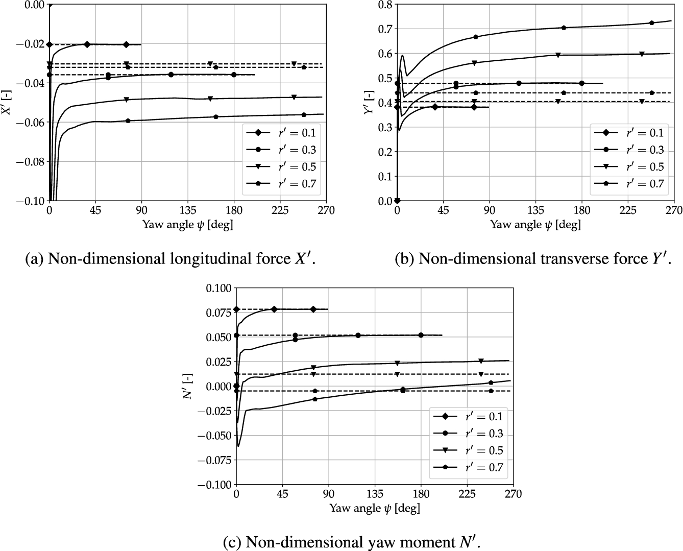
From the observation in Section 3.3 it is known that the two cases with lower rotation rates (r′=0.1 and 0.3) will have the turning circle of the ship interrupted by the domain walls, whereas the cases of the two higher rates will have the entire path of the ship within the computational domain. This fact can be readily observed in the figures: the forces and moment for r′=0.1 and r′=0.3 for the steady approach nicely coincide with the unsteady results after some time (even though it already appears to take around 120 degrees of yaw for the loads in the case of r′=0.3 to stabilise). On the other hand, the steady results of the cases of r′=0.5 and r′=0.7 do not coincide with the unsteady results and the forces are underestimated by up to a factor of two. This consistent underestimation by the steady simulations is a direct result of the disturbed velocity between the vessel and the approaching flow.

For the higher rotation rates it is also visible that a steady state condition of the loads is not attained in the unsteady simulations. In particular for r′=0.7 it can be seen that near the end instead of flattening the curve starts to bend away from an equilibrium. For this turning rate it is very likely that the influence of the wake is already present well before reaching 270 degrees of yaw.

Furthermore, it can be seen that, despite the smooth initial acceleration, the start-up effect takes a substantial amount of time to decay. Simulation attempts with smaller time steps, longer initial acceleration periods or impulsive starts do not seem to improve the initial transient behaviour of the loads significantly.

From these results it can be concluded that the default steady simulation approach underestimates the hydrodynamic forces up to a factor two when the turning circle lies completely within the domain boundaries. Furthermore, despite taking care the unsteady results suffer from start-up influences that progressively linger as the turning rate increases. A secondary observation is that with increasing turning rate a steady state condition of the loads is no longer attained before wake influences start to pollute the measurements. To reliably extract the hydrodynamic loads representative for the steady turn is therefore a non-trivial task for shallow water conditions. In the following, a proposal is made for improved reliability of the computation of steady turning manoeuvres.

4.Wake damping method as proposed solution method

To be able to perform a steady computation in a sufficiently wide domain that includes the full turning circle of a vessel (and thus where wake issues arise), the wake has to be interrupted in some way such that the incoming flow at the bow is undisturbed and uniform again without impacting the hydrodynamic loads on the vessel. It has been noted that a domain boundary forms a natural blockade, but this approach exacerbates wall influences and, moreover, it introduces a dependency between the turning circle and the domain size. Instead, a solution strategy is proposed in which the wake is damped towards the undisturbed flow solution such that its influence on the hydrodynamic loads on the vessel becomes negligible. The damping of the wake is generated by a body force term in the momentum equation that is only applied in a prescribed region in the domain. Because of the geometry of the problem, a sensible shape of this damping zone is a segment of a disc located along the turning circle as shown in Fig. 6.

Fig. 6.

Geometrical definition of the proposed damping zone Dxc (in grey).

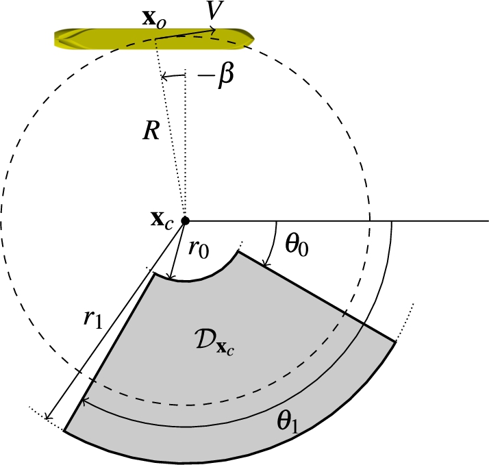
More easily expressed in cylindrical coordinates (r,θ,z) in the computational domain Ω⊂R3 with the origin at the point of rotation xc, a damping zone Dxc⊂Ω in which a restoring body force is applied is defined as:

Here 0⩽r0<r1, 0⩽θ0<θ1⩽2π and the z-values are usually such that the zone continues throughout the complete domain.

The restoring body force is derived by considering the momentum equation in an inertial reference system in conservative form:

Here c is a positive constant without dimension acting as a gain, and 1Dxc:Ω→[0,1] is an indicator function that restricts the contribution of the body force to the interior of the damping zone Dxc. In the present work, the transition across the boundary of the damping zone is chosen to be discontinuous, using a step function 1Dxc=HDxc:Ω→{0,1} defined as:

The application of a discontinuous body force could give rise to concerns relating to stability, but in practice no issues were encountered. Future work nonetheless could entail introducing a smooth indicator function.

The dimensions of the damping zone and the value of the gain c are defined through user input. In this study, the simulation setup is very similar to the configuration in Fig. 6. The vessel is located with respect to xc at an angle of −90−β degrees. Ideally, the damping zone is situated far enough from both the bow and the stern along the turning circle. The inner radius r0 can generally be taken equal to zero without much issue. The value for r1 should be sufficiently large to completely interrupt the wake: in this research r1 always surpasses the domain boundary. Furthermore, all simulations in this study are done with θ0=0 degrees and θ1=60 degrees. These values yield a sector-shaped damping zone that maintains sufficient distance from the bow of the ship to produce an undisturbed incoming flow, while also allowing adequate formation of the wake behind the ship.

Based on our experience with predictions for rotation rates, it is proposed to combine the wake damping method with a sufficiently large domain and application of undisturbed velocity Dirichlet boundary conditions on the far field boundaries. Especially in shallow water, this ensures that the boundary conditions do not contaminate the solution, boundary conditions will be continuous (i.e. there will not be adjacent inflow and outflow faces at locations where the curved flow is locally parallel to the boundary) across the far field, and with the wake damping method, the ship will not encounter its own wake during high rotation rate manoeuvres. Below, this proposed method will be applied.

5.Application of the proposed method

In this section the proposed method of Section 4 is applied and validated11 where possible by comparison with unsteady results. In addition to the case in shallow water conditions of Section 3, a deep water case of the same vessel is considered.

5.1.Validation in shallow water conditions

The set of rotation manoeuvres in shallow water introduced in Section 3 is reconsidered and repeated using the wake damping approach derived in Section 4. The input parameters of the CFD simulations as well as the computational mesh and boundary conditions remain unchanged. The wake damping zone is placed as in Fig. 6 with θ0=0 degrees and θ1=60 degrees. The inner radial value is set to r0=0. The outer radial value r1 and the vertical values z0 and z1 are such that the zone extends beyond the domain boundaries.

Fig. 7.

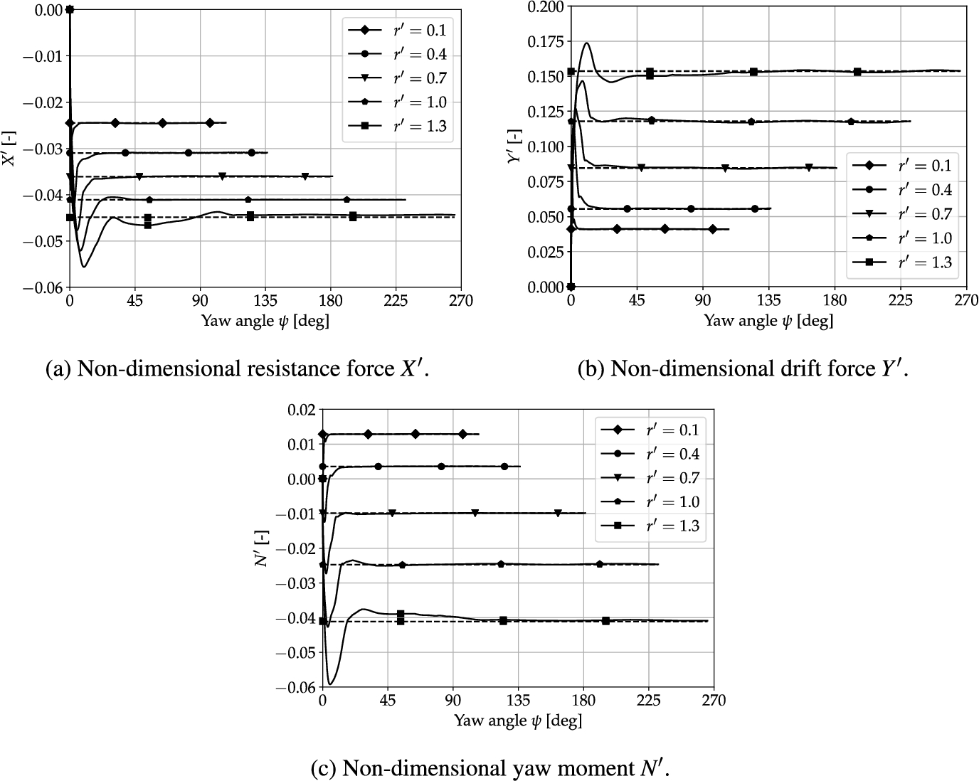
Hydrodynamic loads computed using the proposed approach (dashed lines) as well as the unsteady (solid lines) simulations in shallow water conditions.

The hydrodynamic loads from both the unchanged unsteady results and the results of the proposed approach are presented in Fig. 7. First, it is verified that the results of the lower two yaw rates r′=0.1 and r′=0.3 remain unchanged compared to the default simulations as the starboard domain wall interrupts the sailed path and prevents any wake encounter for these configurations. It is found that the results of the proposed approach differ less than 0.5% from the result from the default approach. This implies that the damping zone has negligible impact on the hydrodynamic loads when enabled but not required.

Fig. 8.

Flow solution u scaled with the sailing velocity in the logarithmic range [0.01,1.5] on the horizontal symmetry plane for r′=0.7 in shallow water conditions.

The efficacy of the proposed steady approach is evaluated by examining the results of the simulations with the two higher yaw rates. In Fig. 8 the resulting flow field is shown for the default (left), unsteady (centre) and the proposed (right) approaches. For the purpose of these kinds of simulations, an undisturbed incoming flow is desired in front of the bow of the ship. The result of the default approach however shows the developed wake directly influencing the incoming flow near the ship. This lowers the effective sailing velocity and thus the hydrodynamic loads. In the right figure, the wake is seen to disperse at some point, and the upstream disturbances near the bow do not appear to result from any wake encounter. The location of the damping zone around the centre of rotation can be readily identified as a 60-degree sector in the lower right quadrant of the circular path, showing a gradual decay of the velocity in the wake.

Compared to the results in Fig. 5 there is now a much better match between the steady and unsteady values for the higher rotation rates of r′=0.5 and r′=0.7. For r′=0.5, the steady values obtained with the proposed approach with wake damping converge to the steady-state results of the unsteady simulations. For the highest yaw rate r′=0.7, the unsteady results do not stabilise to a steady condition, but a reasonable match between the average value of the unsteady results and the proposed approach result is seen. Compared to the default approach, a considerable improvement of the results is therefore obtained. Because the unsteady simulations with the higher rotation rate unfortunately do not show convergence of the results in time, it cannot be concluded that the proposed approach necessarily leads to the correct answers: either more advanced computational techniques or experimental results are needed to be able to draw such conclusions. However, the original aim of devising a technique that allows relatively cheap steady computations to obtain the same results as more expensive unsteady simulations appears to work in those circumstances where unsteady simulations converge nicely. At the very least this provides a level of confidence in the accuracy of the proposed method in cases where the unsteady results do not lead to definite answers.

5.2.Validation in deep water conditions

As a second demonstration of the wake damping method, the MISS in deep water is considered in a computational domain that is typically used for pure drift computations. The domain is rectangular with dimensions 8Lpp×8Lpp×2Lpp. The computational mesh uses the same refinement strategy as the mesh of the shallow domain (with the exception of the local refinement on the bottom) and contains 12.6 million volume cells with 280 thousand faces covering the ship.

Simulations of a rotational manoeuvre with a drift angle of 10 degrees are performed for values of the rotation rate r′ in the range [0.1,1.3]. Since the domain width is 4Lpp, Equation (1) implies that for r′>0.5 the sailed path along the turning circle will be located entirely inside the computational domain. To assess the severity of the wake influence in deep water conditions, a set of steady and unsteady simulations is performed without the proposed wake damping approach (i.e. using the default steady approach to be compared with the unsteady results) first. Boundary conditions and simulation parameters used are identical to the settings of the shallow water example in Section 3.

Fig. 9.

Default steady simulations: iterative convergence of the residuals of the flow equations (top row) and the hydrodynamic force differences ΔX′ and ΔY′ (bottom row) in deep water conditions for the two highest rotation rates.

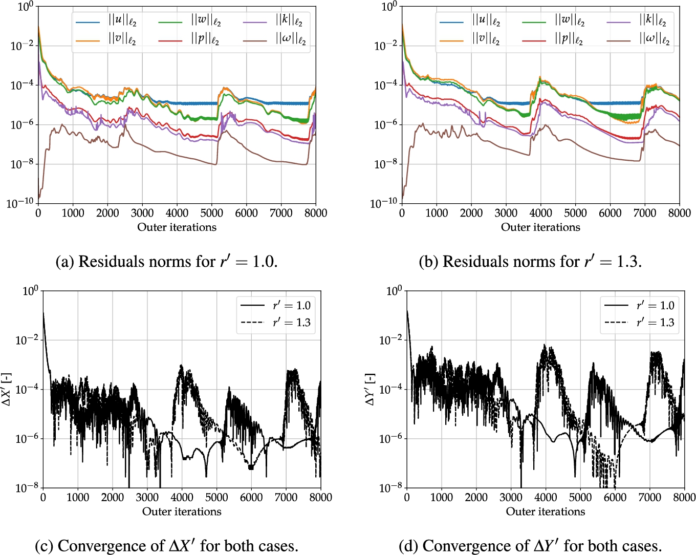
The steady simulations of the cases r′=0.1 and r′=0.4 converge nicely without issues, but the cases with higher yaw rates suffer from noticeable periodicity in both the residuals and the hydrodynamic loads as shown in Fig. 9 for the extreme cases with r′=1 and r′=1.3. The convergence of the hydrodynamic loads is presented as the iterative difference, i.e. ΔXi′=Xi+1′−Xi′ and ΔYi′=Yi+1′−Yi′, for the ith outer iteration. Adjusting simulation settings like relaxation parameters, linear solver accuracy or maximum outer iterations unfortunately does not yield much improvement, and therefore the steady simulations for which the sailed path lies within the domain formally do not converge iteratively. The unsteady simulations on the other hand show consistent convergence of the outer loop at each time step without any further issues.

To investigate whether the use of the proposed approach improves iterative convergence, the steady simulations are performed with the wake damping method enabled. The geometry of the damping zone is identical to the geometry used in the shallow water case of Section 5.1. Aside from enabling the damping zone, all simulation parameters remain unchanged, and the resulting residuals and hydrodynamic forces are shown in Fig. 10.

Fig. 10.

Steady simulations with proposed wake damping: iterative convergence of the residuals of the flow equations (top row) and the hydrodynamic force differences ΔX′ and ΔY′ (bottom row) in deep water conditions for the two highest rotation rates.

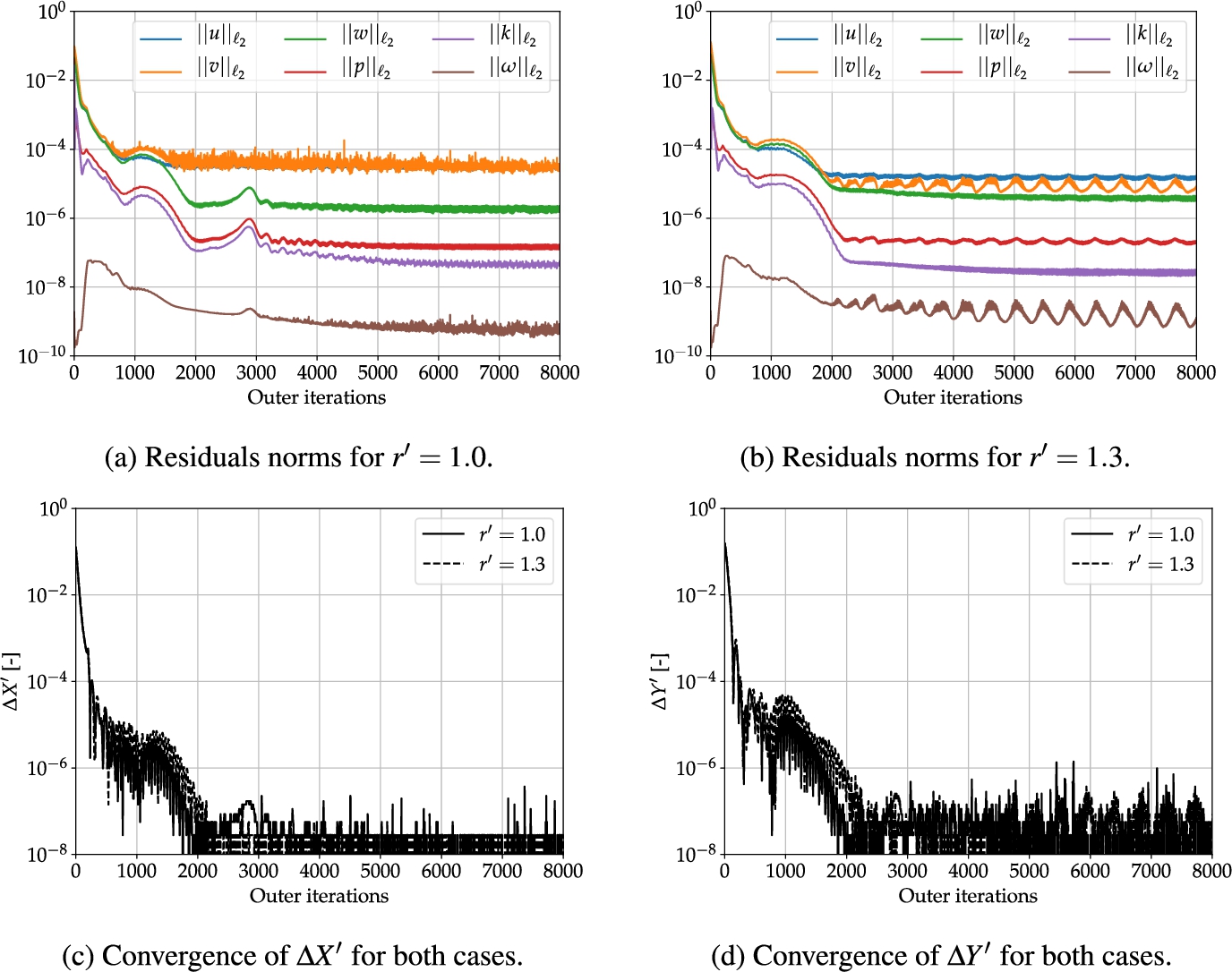
Comparing Fig. 9 and Fig. 10 shows that the proposed method leads to better and more consistent convergence of the residuals even though they all stagnate at some point (which is not an uncommon occurrence on unstructured meshes containing hanging nodes). The extreme case of r′=1.3 is likely close to the limit of the capabilities of a steady approach for this manoeuvre: most residuals show fair convergence but some become noticeably oscillatory. The hydrodynamic forces with the proposed wake damping approach converge much better compared to the default approach, with steady behaviour from around 2500 iterations on. Their stagnation around 10−8 is due to the limited precision of the simulation output.

With the steady simulations now converged for all yaw rates using the wake damping approach, the hydrodynamic loads are compared to the unsteady results in Fig. 11. For the lower yaw rates of r′=0.1 and r′=0.4 an excellent match is expected given the fact that no wake encounter occurs due to the size of the computational domain. Indeed, for these yaw rates the steady and unsteady results for all loads are indistinguishable after the initial acceleration effects have decayed. The simulation results of the higher yaw rates also show a good correspondence of the steady and unsteady loads up to the extreme case of r′=1.3. The unsteady results of the latter case appear to take around 150 degrees of turn to stabilise but the transverse force Y′ and the yaw moment N′ continue to show small fluctuations up to 270 degrees. Nonetheless, the overall match is very satisfactory for a considerable range of yaw rates. The steady simulations with the proposed method are considerably less CPU demanding than the unsteady simulations: for r′=1.3 the steady simulations are about 8 times faster.

Fig. 11.

Hydrodynamic loads computed using the proposed approach (dashed lines) as well as the unsteady (solid lines) simulations in deep water conditions.

The findings from this section and Section 5.1 clearly demonstrate how the proposed approach using wake damping improves both the accuracy (in shallow water conditions) and robustness (in deep water conditions) of steady rotation simulations. It allows the use of a single mesh for all manoeuvring conditions without having to supply suitable meshes that prevent wake encounter for each yaw rate, thus reducing preparation time for the user and increasing consistency between results.

6.Conclusion and recommendations

The present work introduces an efficient and reliable procedure for CFD computations for static yaw manoeuvres as part of the process of establishing a mathematical manoeuvring model. Force or moment coefficients that are a function of the rotational motion are often obtained using steady non-inertial reference frame approaches, assuming negligible influence of free surface deformation. With default approaches as seen in literature, this works well for low rotation rates, but it is demonstrated that steady CFD simulations give results that are fundamentally incorrect when the full turning circle lies within the computational domain, due to the fact that the ship will encounter its own wake. Instead, the turning circle needs to be interrupted by for instance a domain boundary, but this creates a dependency between the domain size and the radius of the turning circle and for large rotation rates the boundaries may influence the flow around the ship, especially in shallow water. To avoid creating new grids for each manoeuvring condition, a simulation method is therefore required that can be applied independently of the domain size and yaw rate. As an alternative, unsteady computations, where only a part of a turning circle is simulated, can be used for rotation cases with high yaw rates, but although they currently yield the most accurate results they are computationally expensive and do not necessarily show convergence towards a time-independent solution of the hydrodynamic loads in shallow water.

To efficiently obtain the hydrodynamic forces and moments acting on a ship in manoeuvring motion, an approach is proposed that utilises a wake damping method. This approach comprises steady computations with a non-inertial reference frame, with the use of a single grid for all manoeuvring conditions, where the boundaries are placed sufficiently far from the ship (4Lpp in deep water and 5Lpp in shallow water) and where consistent boundary conditions (i.e. undisturbed flow) can be applied on all far-field boundaries. With the wake damping method, the wake generated by the ship will be damped to avoid contamination of the undisturbed incoming flow at high rotation rates.

The wake damping method was implemented in the viscous-flow solver ReFRESCO and the proposed approach was demonstrated for manoeuvring conditions in both deep and shallow water. The approach shows favourable convergence properties and good agreement with results from unsteady simulations even for high rotation rates, while computing times are reduced by up to an order of magnitude.

Credit author statement

Guido Oud: Conceptualization, Software, Investigation, Visualization, Writing.

Serge Toxopeus: Methodology, Software, Supervision, Writing.

Conflict of interest

Serge Toxopeus is an Editorial Board Member of this journal, but was not involved in the peer-review process nor had access to any information regarding its peer-review.

References

[1] | B. Alessandrini and G. Delhommeau, Viscous free surface flow past a ship in drift and in rotating motion, in: 22nd Symposium on Naval Hydrodynamics, Fukuoka, Japan, (1998) , pp. 491–507. |
[2] | A. Bedos, G.T. Oud and W. de Boer, Impact of an irregular bank on the sailed trajectory of an inland ship, in: PIANC Smart Rivers Conference, Lyon, France, (2019) . |
[3] | S. Bhushan, H. Yoon, F. Stern, E. Guilmineau, M. Visonneau, S.L. Toxopeus, C.D. Simonsen, S. Aram, S.-E. Kim and G. Grigoropoulos, Assessment of computational fluid dynamic for surface combatant 5415 at straight ahead and static drift |
[4] | L. Bordier, V. Tissot, H. Jasak, V. Vukčevič, G. Rubino, E. Guilmineau, M. Visonneau, G. Papadakis, G. Grigoropoulos, S.L. Toxopeus, F. Stern and S. Aram, Assessment of Prediction Methods for Large Amplitude Dynamic Manoeuvres for Naval Vehicles, Chapter 4: DTMB-5415 Pure Sway Simulations, NATO TR-AVT-253 Report, 2021. |
[5] | P.M. Carrica, F. Ismail, M. Hyman, S. Bhushan and F. Stern, Turn and zigzag maneuvers of a surface combatant using a URANS approach with dynamic overset grids, Journal of Marine Science and Technology 18: (2) ((2013) ), 166–181. doi:10.1007/s00773-012-0196-8. |
[6] | A. Cura Hochbaum, Computation of the turbulent flow around a ship model in steady turn and in steady oblique motion, in: 22nd Symposium on Naval Hydrodynamics, Fukuoka, Japan, (1998) , pp. 550–567. |
[7] | A. Cura Hochbaum, M. Vogt and S. Gatchell, Manoeuvring prediction for two tankers based on RANS simulations, in: SIMMAN Workshop on Verification and Validation of Ship Manoeuvring Simulation Methods, Copenhagen, Denmark, (2008) , pp. F23–28. |
[8] | A. Di Mascio, R. Broglia and R. Muscari, Unsteady RANS simulation of a manoeuvring ship hull, in: 25th Symposium on Naval Hydrodynamics, St. John’s, Newfoundland and Labrador, Canada, (2004) , pp. 9–18. |
[9] | L. Eça, C.M. Klaij, G. Vaz, M. Hoekstra and F.S. Pereira, On code verification of RANS solvers, Journal of Computational Physics 310: ((2016) ), 418–439. doi:10.1016/j.jcp.2016.01.002. |
[10] | V. Ferrari and F.H.H.A. Quadvlieg, Preliminary considerations on a unified model for hydrodynamic forces, in: 3rd International Conference on Maritime Technology and Engineering (MARTECH), Lisbon, Portugal, (2016) . |
[11] | A. Franceschi, B. Piaggio, R. Tonelli, D. Villa and M. Viviani, Assessment of the Manoeuvrability Characteristics of a Twin Shaft Naval Vessel Using an Open-Source CFD Code, Journal of Marine Science and Engineering 9(6) (2021). doi:10.3390/jmse9060665. |
[12] | T. Gao, Y. Wang, Y. Pang, Q. Chen and Y. Tang, A time-efficient CFD approach for hydrodynamic coefficient determination and model simplification of submarine, Ocean Engineering 154: ((2018) ), 16–26. doi:10.1016/j.oceaneng.2018.02.003. |
[13] | M. Garenaux, A. de Jager, H.C. Raven and C. Veldhuis, Shallow-water performance prediction: Hybrid approach of model testing and CFD calculations, in: 14th International Symposium on Practical Design of Ships and Other Floating Structures (PRADS), Yokohama, Japan, (2019) , pp. 63–82. doi:10.1007/978-981-15-4624-2_4. |
[14] | A.G.L. Holloway, T.L. Jeans and G.D. Watt, Flow separation from submarine shaped bodies of revolution in steady turning, Ocean Engineering 108: ((2015) ), 426–438. doi:10.1016/j.oceaneng.2015.07.052. |
[15] | ITTC – Recommended Procedures and Guidelines, Guideline on the Use of RANS Tools for Manoeuvring Predictions, 2017. |
[16] | C.M. Klaij and C. Vuik, SIMPLE-type preconditioners for cell-centered, colocated finite volume discretization of incompressible Reynolds-averaged Navier-Stokes equations, International Journal for Numerical Methods in Fluids 71: (7) ((2013) ), 830–849. doi:10.1002/fld.3686. |
[17] | L. Larsson, F. Stern and M. Visonneau (eds), Gothenburg 2010: A Workshop on Numerical Ship Hydrodynamics, Gothenburg, Sweden, (2010) . |
[18] | L. Larsson, F. Stern, M. Visonneau, N. Hirata, T. Hino and J. Kim (eds), in: Tokyo 2015, a Workshop on CFD in Ship Hydrodynamics, Tokyo, Japan, (2015) . |
[19] | F.R. Menter, Y. Egorov and D. Rusch, Steady and Unsteady Flow Modelling Using the k- |
[20] | T.F. Miller and F.W. Schmidt, Use of a pressure-weighted interpolation method for the solution of the incompressible Navier-Stokes equations on a nonstaggered grid system, Numerical Heat Transfer 14: (2) ((1988) ), 213–233. doi:10.1080/10407788808913641. |
[21] | NATO AVT-183 Task Group, Reliable Prediction of Separated Flow Onset and Progression for Air and Sea Vehicles, NATO TR-AVT-183 Report, 2017. |
[22] | NATO AVT-253 Task Group, Assessment of Prediction Methods for Large Amplitude Dynamic Manoeuvres for Naval Vehicles, NATO TR-AVT-253 Report, 2021. |
[23] | T. Ohmori, Finite-volume simulations of flows about a ship in manoeuvring motion, Journal of Marine Science and Technology 3: (2) ((1998) ), 82–93. doi:10.1007/BF02492563. |
[24] | C. Oldfield, M. Moradi Larmaei, A. Kendrick and K. McTaggart, Prediction of warship manoeuvring coefficients using CFD, in: World Maritime Technology Conference (WMTC), Providence, RI, (2015) . |
[25] | G.T. Oud and A. Bedos, CFD investigation of the effect of water depth on manoeuvring forces on inland ships, in: IX International Conference on Computational Methods in Marine Engineering (MARINE), (2021) . |
[26] | J.-H. Park, M.-S. Shin, Y.-H. Jeon and Y.-G. Kim, Simulation-based prediction of steady turning ability of a symmetrical underwater vehicle considering interactions between yaw rate and drift/rudder angle, Journal of Ocean Engineering and Technology 35: (2) ((2021) ), 99–112. doi:10.26748/KSOE.2020.067. |
[27] | F.H.H.A. Quadvlieg, C.D. Simonsen, J.F. Otzen and F. Stern, in: Review of the SIMMAN2014 Workshop on the State of the Art of Prediction Techniques for Ship Manoeuvrability, in: International Conference on Ship Manoeuvrability and Maritime Simulation (MARSIM), Newcastle, UK, (2015) . |
[28] | F.H.H.A. Quadvlieg, F. Stern, C.D. Simonsen and J. Flensborg, in: SIMMAN Workshop on Verification and Validation of Ship Manoeuvring Simulation Methods, Otzen, ed., Copenhagen, Denmark, (2014) . |
[29] | H.C. Raven, A computational study of shallow-water effects on ship viscous resistance, in: 29th Symposium on Naval Hydrodynamics, Gothenburg, Sweden, (2012) . |
[30] | P.J. Roache, Fundamentals of Verification and Validation, Hermosa Publishers, (2009) . ISBN 978-0-913478-12-7. |
[31] | S.L. Toxopeus, Validation of slender-body method for prediction of linear manoeuvring coefficients using experiments and viscous-flow calculations, in: 7th ICHD International Conference on Hydrodynamics, Ischia, Italy, (2006) , pp. 589–598. |
[32] | S.L. Toxopeus, Practical Application of Viscous-Flow Calculations for the Simulation of Manoeuvring Ships, PhD thesis, Delft University of Technology, Faculty Mechanical, Maritime and Materials Engineering, 2011. |
[33] | S.L. Toxopeus, P. Atsavapranee, E. Wolf, S. Daum, R.J. Pattenden, R. Widjaja, J.T. Zhang and A.G. Gerber, Collaborative CFD exercise for a submarine in a steady turn, in: 31st International Conference on Ocean, Offshore and Arctic Engineering (OMAE), Rio de Janeiro, Brazil, (2012) . doi:10.1115/OMAE2012-83573. |
[34] | S.L. Toxopeus, K. Hoyer, M. Tenzer, B. Friedhoff, G.T. Oud, D. Boucetta and J.W. Settels, Vessel Train Hydrodynamics, NOVIMAR Deliverable 3.4, 2020. |
[35] | S.L. Toxopeus, H. Jasak, E. Guilmineau, L. Bordier, G. Papadakis, S. Aram, F. Stern, M. Visonneau, V. Vukčevič, G. Rubino, V. Tissot and G. Grigoropoulos, Assessment of Prediction Methods for Large Amplitude Dynamic Manoeuvres for Naval Vehicles, Chapter 3: CFD Validation for Surface Combatant 5415 at 10° Drift Angle, NATO TR-AVT-253 Report, 2021. |
[36] | S.L. Toxopeus and S.W. Lee, Comparison of manoeuvring simulation programs for SIMMAN test cases, in: SIMMAN Workshop on Verification and Validation of Ship Manoeuvring Simulation Methods, Copenhagen, Denmark, (2008) , pp. E56–61. |
[37] | N.P. Waterson and H. Deconinck, Design principles for bounded higher-order convection schemes – a unified approach, Journal of Computational Physics 224: (1) ((2007) ), 182–207. doi:10.1016/j.jcp.2007.01.021. |
[38] | P. Wesseling, Principles of Computational Fluid Dynamics, Springer-Verlag, (2000) . ISBN 3-540-67853-0. |
[39] | X. Wu, Y. Wang, C. Huang, Z. Hu and R. Yi, An effective CFD approach for marine-vehicle maneuvering simulation based on the hybrid reference frames method, Ocean Engineering 109: ((2015) ), 83–92. doi:10.1016/j.oceaneng.2015.08.057. |
[40] | J.T. Zhang, J.A. Maxwell, A.G. Gerber, A.G.L. Holloway and G.D. Watt, Simulation of the flow over axisymmetric submarine hulls in steady turning, Ocean Engineering 57: ((2013) ), 180–196. doi:10.1016/j.oceaneng.2012.09.016. |