Experimental and numerical assessment of vertical accelerations during bow re-entry of a RIB in irregular waves

van der Eijk, Martin; Wellens, Peter

doi:10.3233/ISP-201005

Experimental and numerical assessment of vertical accelerations during bow re-entry of a RIB in irregular waves

Article type: Research Article

Authors: van der Eijk, Martin | Wellens, Peter^{; *}

Affiliations: Delft University of Technology, Mekelweg 2 2628CD Delft, The Netherlands

Correspondence: [*] Corresponding author. E-mail: [email protected].

Keywords: Ship model test, irregular waves, high speed craft, bow re-entry, CFD, multiphase flow

DOI: 10.3233/ISP-201005

Journal: International Shipbuilding Progress, vol. 67, no. 2-4, pp. 173-198, 2020

Received 13 October 2020

Revision received 22 April 2021

Accepted 23 April 2021

Published: 7 July 2021

Get PDF

Abstract

This paper presents the comparison of a self-conducted towing tank experiment with the simulation results of a calibrated state-of-the-art strip-theory method and a first-principles numerical method. The experiment concerns a Rigid Inflatable Boat (RIB) in moderate-to-high irregular waves. These waves result in bow emersion events of the RIB. Bow re-entry induces vertical accelerations which, in reality, can lead to severe injuries and structural damage. State-of-the-art methods for predicting the vertical acceleration levels are based on assumptions, require calibration and are often limited in application range. We demonstrate how the vertical acceleration as a function of time is found from a 3D numerical method based on the Navier–Stokes equations, employing the Volume of Fluid (VoF) method for the free surface, without any further assumptions or limitations.

2D+t strip theory methods like Fastship are based on the mechanics of wedges falling in water. The 3D numerical method that is part of the software ComFLOW is compared to previous research on falling wedges in 2D to investigate the effect of air and to find suitable grid distances for the 3D simulation of the RIB. The 3D RIB simulations are compared to Fastship and the experiment. With respect to the experiment, the ComFLOW simulations show a slight underestimation of the levels of heave and pitch. The underestimation of Fastship is larger. The prediction of acceleration in ComFLOW is hardly different from the experiment and a significant improvement with respect to Fastship. ComFLOW is demonstrated to predict acceleration levels better than before, which creates opportunities for using it in seakeeping optimization and for the improvement of methods like Fastship. The properties of the RIB and the experiment are available as open data at Wellens (2020).

1.Introduction

After a comprehensive study of U.S. Special Operations craft crewmen, 62% of the crew reported one or more injuries that required hospitalization attributed to high-speed craft operation (Peterson et al. [19]). The demand for high speed craft to be operational under all weather conditions without injuries leads to harsh design restrictions where bow emergence and re-entry play an important role. Bow re-entry in reality can lead to high vertical accelerations. In earlier years, reduction of the total resistance to reach the highest forward speed was the main objective. This resulted in adverse seakeeping behavior where the impacts induce severe injuries to the crew. Measurements aboard Fast Raiding Interception and Special forces Craft (FRISC) showed that acceleration pulses up to 15g were achieved (Marges [16]). Van Deyzen [24] concluded based on full scale trial data that the repeated occurrence of 1g vertical acceleration was acceptable for the crew. To prevent injury and structural damage following these high accelerations, the operator needs to reduce speed. Speed-adaptation results in a reduced operational profile.

To enlarge the operational profile at high speeds and reduce the vertical accelerations, the performance of the craft can be increased by improved ship design, the design subsequently evaluated by conducting experiments that test the sea keeping behavior. In support of experiments, approximating mathematical and numerical methods for predicting accelerations have been developed over the years, among which Fastship (Keuning [12]). The state-of-the-art of these methods is limited in its range of application, because they depend, in part, on simplifications and calibrated empirical relations.

Here, we propose a first-principles numerical method to predict the acceleration levels of a Rigid Inflatable Boat (RIB) in moderate-to-high irregular waves. From what we were able to find in literature, the main contribution of this article is a direct deterministic comparison of vertical acceleration in time in irregular waves between 3 methods: self-conducted towing tank experiments, a calibrated state-of-the-art strip theory method called Fastship, and a 3D method based on the Navier–Stokes equations called ComFLOW (Kleefsman et al. [13]). The comparison is done for the entire time that a model is at constant speed in a run.

High speed craft have been widely investigated with most of the mathematical/numerical studies being based on slender body assumptions or potential theory (Zhao [33], Lai et al. [14]). Fundamental work regarding the nonlinear periodic change in wetted area of a slender object in waves was done by Bos and Wellens [2]. Several approaches to predict the performance of a high speed craft in calm water exist in literature. Tavakoli et al. [21] developed a mathematical model for the performance of planing hulls in forward accelerating motion. The model is extended with empirical equations of displacement ships and 2D+t theory, showing a fair agreement with experimental results. Recent numerical work of Broglia and Durante [3] focused on the challenging free surface flow problem involving a surface vessel at high speeds in calm water using a numerical one-phase uRaNS flow solver. They mentioned that the application of a CFD based approach to study high speed craft is still rather limited. An experimental and numerical study of the total resistance and drag prediction is done by Avci and Barlas [1]. They conducted a towing tank test with a high speed hull to compare with CFD methods, resulting in a good agreement for the total resistance.

There are few accounts of validated 3D numerical approaches to predict the vertical accelerations of high speed craft in irregular waves in literature. Wang et al. [25] performed numerical simulations of a planing craft in regular waves using a RaNSE VoF solver where they focused on the sea keeping performance instead of the resistance. They concluded that validation with a model or full-scale measurement still remains of the essence. Mousaviraad et al. [17] assessed the capability of URaNS for the hydrodynamic performance and bow re-entry of a high speed craft. Simulations of a high speed craft in regular as well as irregular low-to-moderate waves were performed at a Froude number of 1.8–2.1. The results were validated with experiments for the mean and amplitudes of resistance, heave, pitch and acceleration. Similarly, Fu et al. [9] performed simulations at the same conditions finding generally good agreement in terms of expected values and standard deviations of vertical acceleration. Furthermore, they analyzed and validated the bow re-entry performance of the craft at high speed including vertical accelerations. More work where the accelerations of a RIB in irregular waves are predicted is done by Lewis et al. [15]. They used a RaNSE model in combination with non-linear strip theory through calculation of the forces occurring on a wedge impact. While the occurrence of wedge impact and the frequency of heave an pitch motions were predicted well, the magnitudes of accelerations were over-predicted compared to experimental data. Articles that deterministically compare the full time registration of the motions containing a bow re-entry event between a first-principles numerical model and an experiment have not been found.

Based on the remarks made by Wang et al. [25] and others, we conducted a towing tank experiment of a RIB in moderate-to-high irregular waves at Froude number Fn≈0.25–1.0 for validation of numerical models. During the experiment, the RIB is restricted to the heave and pitch motion while being towed through the tank at a constant speed. The heave and pitch motion, accelerations and wave height were measured for the time of a run. The experiments were controlled in such a way that in every run a bow emergence and re-entry event was experienced.

The 2D+t method Fastship is compared to the experiment at model scale for the same incoming waves as in the experiment. Fastship is a faster-than-real-time model which makes use of 2D strips of wedges distributed over the hull length. The coefficients for the equation of motion are based on experimental results and analytical relations. The method has been extended over the years to include the effect of control systems for the forward velocity (Rijkens [20], Van Deyzen [24]). Fastship has been used for the design of a RIB in Keuning et al. [11].

The proposed first-principles numerical method in this paper for the hydrodynamic loads on the RIB and the RIB’s motion in waves, is ComFLOW. Structural aspects of the RIB were not considered, although a first step regarding the nonlinear dynamics of plates prestressed by a hydrostatic pressure and superimposed varying loads like in waves was made in Xu and Wellens [30]. 3D simulations of the RIB motions using ComFLOW are performed at the same scale and circumstances as the conducted experiment. Again, the incoming waves are the same as in the experiment. The numerical method ComFLOW has been under development since Fekken et al. [8]. Over the last few years, research is done to improve the description of violent flow phenomena which are both highly non-linear and highly dispersive (Gerrits [10], Kleefsman et al. [13], Wemmenhove [29], Van Der Eijk and Wellens [22]). ComFLOW is based on the Navier–Stokes equations for the motion of an aggregated fluid with varying properties. A fixed Cartesian grid is used with a staggered configuration of variables within a cell. The free surface is displaced using the Volume-of-Fluid (VoF) method where the interface is reconstructed using piecewise-linear line segments (PLIC). Using a cut-cell method, a body can be incorporated to determine the interaction with the fluid (Fekken [7]). Validation of the numerical simulation method ComFLOW with experimental data of a RIB in 3D has not been done before.

This article first presents the governing equations of fluid flow that Fastship and ComFLOW are based on. Then, in order to study the importance of air and to find the appropriate grid configuration for the prediction of bow re-entry, free falling wedge drop tests are simulated with ComFLOW. By conducting the wedge drop simulations, a first experience of how ComFLOW behaves for simplified bow entries is demonstrated. With the selected grids, 3D simulations with the RIB are performed. At the end, the comparison between the experiment, Fastship and ComFLOW is made and conclusions are formulated based on the results. The details of the RIB and the experiment are provided as open data, see Wellens [27].

2.Governing equations

2.1.One-phase flow model

The one-phase flow model makes use of the assumption that the effect of air can be neglected. Water is considered as an incompressible and viscous liquid. Air is considered as a vacuum. The liquid motion in a 3D domain is described by the Navier–Stokes equations and a fluid displacement algorithm. For the one-phase flow model, the governing equations are only applied in the liquid-filled part of the domain. The Navier–Stokes equations are simplified to (Gerrits [10])

(1)∇·u=0,∂u∂t+u·∇u=−1ρ∇p+μρ∇2u+F,

with u the velocity vector, ρ the density of the fluid, p the pressure and μ the dynamic viscosity. F are the external body forces, in this case only gravity; [00−9.81]T[m/s2]. For an incompressible flow, the density does not change in a lagrangian manner and therefore the divergence of the velocity is zero.

2.2.Two-phase flow model

In contrast to the one-phase flow model, the two-phase flow model solves for water and air in the entire domain, making it more computationally expensive. In this model water remains an incompressible, viscous fluid. Air is chosen as a compressible viscous fluid to account for cushioning effects.

The Navier–Stokes equations are stated for a mixed fluid in which the pressure is relaxed to a single field. This results in one continuity and one momentum equation for both water and air (Wemmenhove [29])

(2)∂ρ∂t+∇·(ρu)=0,∂(ρu)∂t+∇·(ρuu)=−∇p∂(ρu)∂t+∇·(ρuu)=+∇·(μ(∇u+∇uT−23∇·uI))∂(ρu)∂t+∇·(ρuu)=+ρF.

The mixed fluid properties ρ and μ are defined in Eq. (7). To close the system of equations, an energy equation referred to as the equation of state is introduced

(3)ppref=(ρgρg,ref)γ.

Equation (3) is a polytropic relation between the pressure and density of the compressible gas. p and ρg are the pressure and density of the compressible air. pref is the atmospheric pressure and ρg,ref is the air density at atmospheric pressure. γ is the adiabatic coefficient: γ=1.4 for air is used.

2.3.Free surface & boundary conditions

For both the one-phase and the two-phase model, the fluid displacement algorithm is described by a function s(x,t)=0, with x=(x,y,z)T. The equation of the displacement of the free surface is as follows (Gerrits [10])

(4)DsDt=∂s∂t+u·∇s=0.

The boundary conditions needed by both models are as follows. At the fixed walls of the domain and at boundaries of moving objects, no penetration boundary conditions are applied, u·n=0 and u·n=ub·n, respectively. At domain walls also a free-slip boundary condition is imposed, τ·n. ub is the velocity of the moving object. When performing wave simulations, an inflow boundary is needed where the velocity profile of the incoming wave is prescribed and an outflow boundary for the absorption of waves. To that end, the Generating and Absorbing Boundary Condition (GABC) of Wellens and Borsboom [28] is used in combination with the superposition of linear wave velocity components to model an irregular wave. The settings of the GABC are elaborated upon in Section 5.

In only the one-phase flow model, boundary conditions for pressure and velocity are needed at the free surface to close the system. Equations (5) and (6) are the result of continuity of the normal and tangential stresses (Gerrits [10]) at the free surface

(5)−p+2μ∂un∂n=−p0+σκ,(6)μ(∂un∂t+∂ut∂n)=0,

where un and ut denote the normal and tangential component of the velocity. p0 is the atmospheric pressure.

The two-phase flow model requires the atmospheric pressure to be set at a boundary that only connects with air, usually the ceiling of the domain.

3.Numerical discretisation

3.1.Cell labelling

The mathematical model is implemented in the pressure-based numerical solution method ComFLOW. In order to solve the Navier–Stokes equations, the computational domain is covered with a fixed and staggered Cartesian grid. In the grid, pressure and density are defined in cell centers and velocities are defined at the edges of the cell. The Navier–Stokes equations are solved in every cell (or in every cell that contains water in one-phase simulations). Structure geometries cut through the grid so that cells within the contour of the structure are partially or completely closed to flow. We call those cut cells and they are administered by edge and volume apertures. The apertures are a measure for which part of the cell face or cell volume is open to flow.

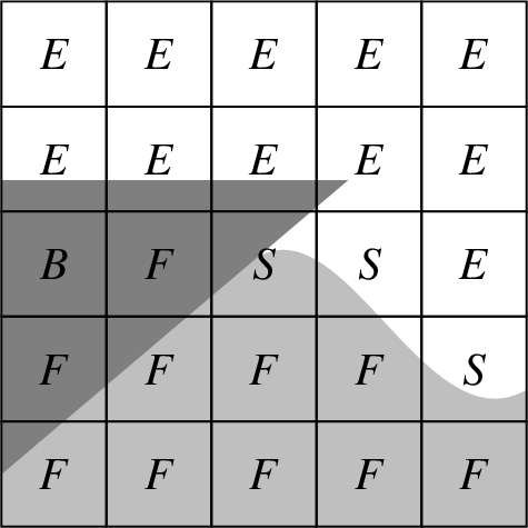
The cells are divided into three groups to describe the fluid configuration. Cells which can be filled with water, but are filled with air (or empty in one-phase), are called E-cells. A S-cell (surface) contains fluid and is next to an E-cell. The remaining cells containing fluid are labelled with F. Cells which are fully occupied by the structure are labelled with B. An example of the labelling is illustrated in Fig. 1.

Fig. 1.

Labelling of cells.

3.2.Discretisation of the Navier–Stokes equations

Where for the one-phase flow model the density and viscosity do not change, with the two-phase flow model they do because of the aggregate fluid assumption and the effect of compressibility. Density values are defined in the centers of cells and found by arithmetic averaging

(7)ρ=FsFbρl+Fb−FsFbρg,μ=FsFbμl+Fb−FsFbμg,

where Fb and Fs are the fractions of the cells that are open for flow and occupied with liquid, respectively. The water density ρl remains constant and the air density is calculated using Eq. (3). At the cell faces the density and viscosity are calculated by cell-weighted averaging (Van Der Eijk and Wellens [22]).

Velocities near and above the free surface are not solved for in the one-phase approach. These so-called EE and SE velocities, see Fig. 1, are needed to complete the discretisation of the convective term in the momentum equation. They are found by constant extrapolation from the inside of the water (Kleefsman et al. [13]).

To solve the Navier–Stokes equations, the equations are discretised in time and space. The combination of the forward Euler method for time integration and central discretisations of the derivatives in space is used for all but the non-linear convective term. In that term, a first order upwind discretisation is used. The forward Euler method is a first order method but accurate enough, because of small time steps and because the overall accuracy is determined by the accuracy of the free surface displacement (Kleefsman et al. [13]). No eddy viscosity model is used.

The system is solved using a one-step projection method. A Poisson equation is formulated and solved for the pressure with a BiCGSTAB solver (Van der Vorst [23]), with ILU(ε) preconditioning. This solver is compatible with both one-phase flow and two-phase flow and sufficiently robust for the large density variations from air to water near the free surface in two-phase flow simulations. The free surface is convected by the improved Volume-of-Fluid (iVOF) method in ComFLOW: the free surface is reconstructed using a Piecewise Linear Interface Calculation (PLIC, Youngs [31]) and displaced with the split scheme MACHO (Duz [5]) to solve Eq. (4). A Courant number (CFL) restriction, based on the velocity u, is used for numerical stability.

In ComFLOW, we choose to keep the motion solver for the structure separate from the Poisson equation so that we can link to external libraries. That creates a difficulty: the body velocities are required at the new time step, but they depend on the pressures along the hull, and the new pressures along the hull depend on the new body velocities. The two-way coupling between structure and fluid is solved iteratively with underrelaxation applied to the update of the body velocities, that consists of body force over mass of the structure. Tangential stresses are ignored in the body force calculation.

4.Simulation of wedge entry compared with experiment

Water-entry of a wedge shaped section has been investigated in numerous studies, e.g. numerically in 2D and 3D by [13] and experimentally in 3D by [34]. Wedge entry is a simplification of a bow re-entry event and often used for the prediction of the forces on a cross section in a 2D strip theory approach for a ship. We use falling wedges to verify ComFLOW, to determine which physics are relevant for the 3D case, and for finding the grid resolution. The geometry of the wedge is shown in Fig. 2. The size of the cross section is similar to the 3D RIB. Besides 2D simulations of the wedge entry also a 3D simulation is done to compare with the 3D experimental data of Zhao et al. [34]. Muzaferija [18] determined that a gap of 0.25 m between the back and front wall and the wedge in the 3D simulation gives results that compare well with experiments.

Fig. 2.

Domain and dimensions of the wedge in [m].

4.1.Setup wedge entry

The domain, illustrated in Fig. 2, has the same dimensions that were used in the experiment by Zhao et al. [34]. The water depth is 1.5 m. The free falling wedge moves in vertical direction and has an impact velocity at the water surface of 6.15 m/s. In the one-phase simulations the wedge is simulated with an initial speed of 6.13 m/s and a starting location 0.015 m above the water surface. The initial speed has been calculated using conservation of energy.

For the two-phase flow simulations, the setup is largely the same as with one-phase. In order to investigate the relevance of compressible air on wedge entries, the wedge is positioned 0.1 m above the water surface to be able to develop the air cushioning effect (Bullock et al. [4]). Again the initial velocity is calculated using conservation of energy, taking into account a margin for the air resistance. The initial speed is set at 5.99 m/s.

The boundary condition at the top of the domain with air defines the atmospheric pressure. For the simulation it is critical to have a small time step at the time the wedge enters the water surface so that the impact is represented accurately. For all simulations a maximum CFL restriction of 0.7 is used, enforcing smaller time steps when fluid velocities become higher. The time step is never larger than 0.001 s.

4.2.Appropriate grid resolution 2D wedge entry

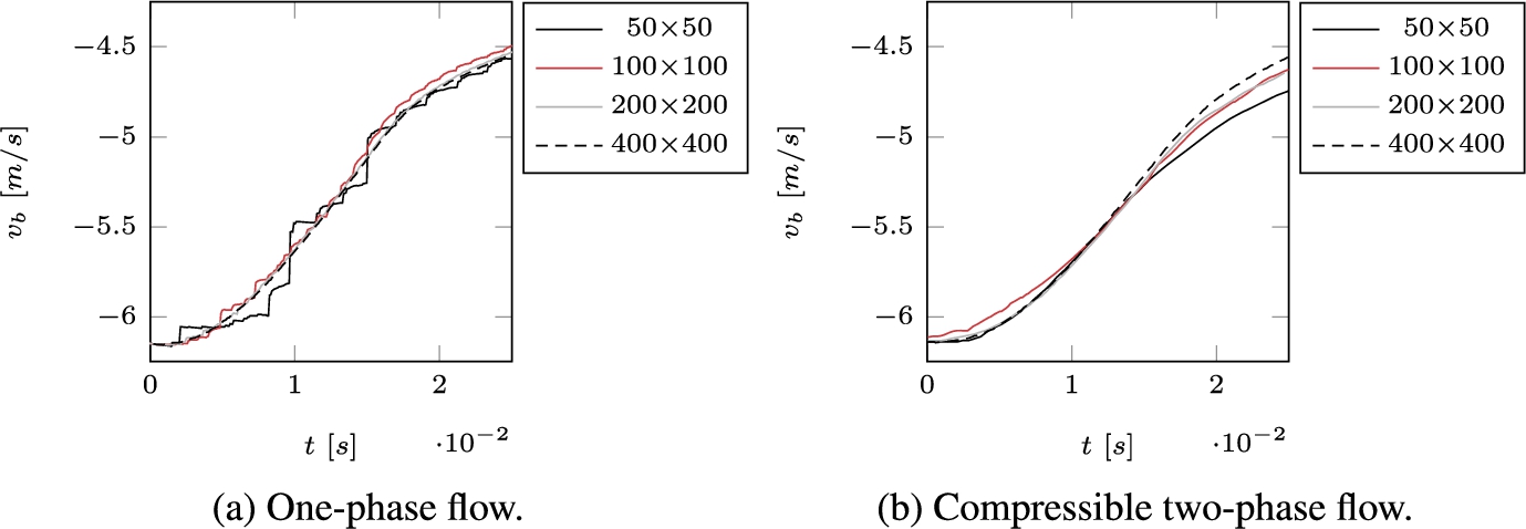
In order to determine which grid size is suitable for the simulation of the RIB in the following section, a grid convergence study has been done for the one-phase flow model as well as the two-phase flow model in ComFLOW. In Figs 3a and 3b the velocity of the wedge over time is plotted. With the grid 50×50 we capture the width of the RIB with around 8 cells.

The one-phase flow model shows jumps in the vertical speed which depend on the grid resolution. These jumps in the speed are related to label changes. The label defines whether the free surface conditions in Eqs (5) and (6) need to be enforced. The resulting discontinuous pressure in time affects the vertical velocity of the wedge through its equation of motion. The vertical velocity is smoothened by grid refinement due to the smaller effect of local pressures on the global motion. Figure 4 also shows that true grid convergence is not feasible for the discontinuity of the wedge going from dry to wet. This is in agreement with for instance the dam break simulations in Kleefsman et al. [13]. Grid refinement results in new flow features. These features affect the vertical motion, which can be observed for the two-phase 400×400 grid in Fig. 3b.

Fig. 3.

Wedge entry: 2D grid convergence.

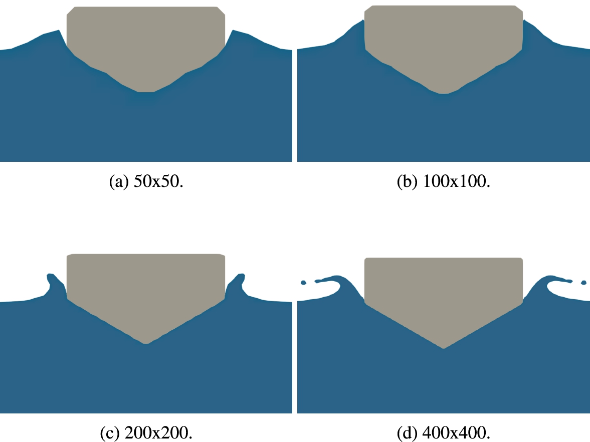
In Fig. 4 the free surface deformation due to the wedge entry is shown for different grid resolutions of the one-phase flow simulations. It shows that the free surface keeps developing new flow features. For the one-phase flow simulations, however, the flow features do not affect the vertical velocities of the wedge as much as for the two-phase simulations. The computational effort of extrapolating the finest grid resolution in Fig. 3 to 3D is too high to be feasible. For this reason, we choose to focus on representing the motions of the RIB well with 50×50 and 100×100 grid cells in the cross-section of the domain, and accept that the free surface near the ship is underresolved.

Fig. 4.

Wedge entry in water with one-phase model at t=0.025 s.

4.3.Comparison one-phase & two-phase flow 2D wedge entry

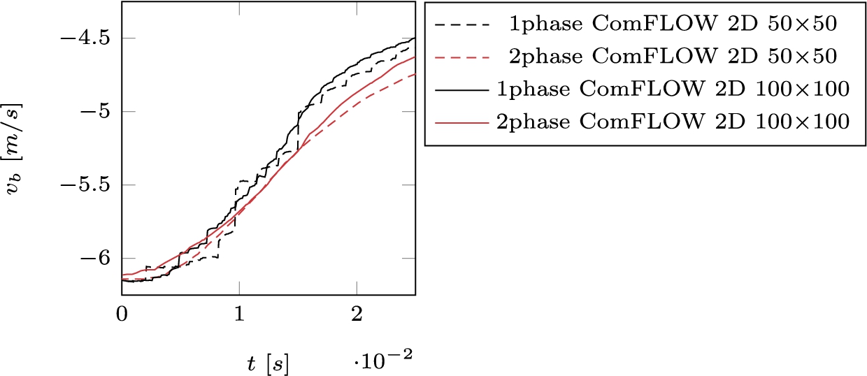
Figure 3a and Fig. 3b show that higher grid resolutions lead to lower differences between the one-phase results. The two finest two-phase results are more different than the two finest one-phase results. The comparison of a wedge entry in one-phase and two-phase for similar resolutions is shown in Fig. 5. Where for the one-phase model only the liquid is solved, the two-phase model using extra equations for the density is solved over the entire domain. This makes the two-phase model more computationally expensive. The difference in computational time is a factor 10 approximately. The one-phase results are so close to the two-phase results that it leads to the conclusion that the computational costs outweigh the benefit of including air effects. This conclusion was not unexpected, Faltinsen [6] concluded that the air cushion effect has an influence on the velocity for deadrise angles of only a few degrees whereas the wedge and the RIB in this study have deadrise angles of 30 degrees or larger. Two-phase is also more dissipative for wave propagation (Wemmenhove [29]). With this in mind we choose to simulate the RIB in 3D without the effect of air.

Fig. 5.

Wedge entry: comparison of one-phase and two-phase flow in 2D.

4.4.Results 3D wedge entry

The comparison of 3D wedge entry simulations on a 50×50×50 and 100×100×100 grid with the 3D experiment of (Zhao et al. [34]) is made in Fig. 6. The 3D one-phase flow simulation results overpredict the deceleration compared to the experimental result. However, the 2D simulations in Fig. 5 overpredict the deceleration significantly more. This is the result of the restricted movement of the fluid and 3D effects. This could mean that the deceleration in 2D strip theory simulations of ships in waves is also exaggerated, which would lead to lower motions and inaccurate predictions of the vertical acceleration. Further, the velocity jumps in 3D are smoothened because the local pressure jumps have less effect on the global velocity of the wedge.

Figure 6 also shows the 3D one-phase simulation done by Kleefsman et al. [13] with a previous version of ComFLOW using a grid of 60×60×60. The new ComFLOW results are similar to ones from the previous version.

Fig. 6.

Wedge entry: comparison of 3D one-phase with experiment.

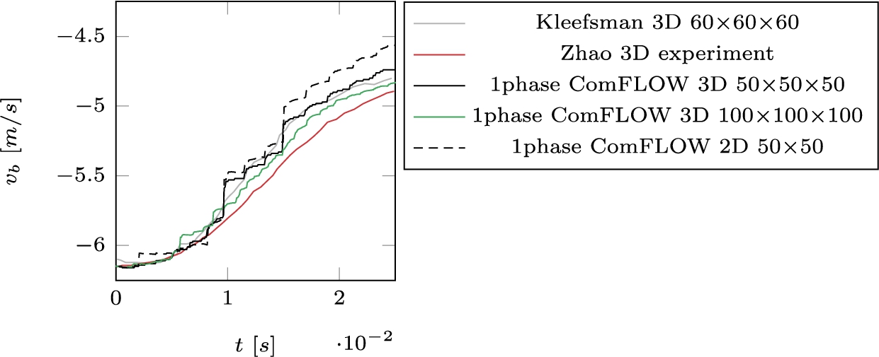
Based on the investigation with falling wedges, 1 phase simulations with a minimum of 8 cells along the width of the RIB are appropriate to represent its vertical motion behavior.

5.3D simulations with Fastship and ComFLOW compared with experiment

An experiment with a RIB was conducted specifically for the purpose of this article in the small towing tank of the Ship Hydromechanics Laboratory at Delft University of Technology. The main objective of the experiment was to generate a bow emergence and re-entry event in each run; to that end the highest surface elevation in a sea state defined by a JONSWAP spectrum with a set peak period and significant wave height, would be met by the RIB at the desired velocity in a specific location in the tank. That specific location was 50 m away from the wave board, where even for the highest velocity it was certain that the boat had accelerated to meet the desired velocity. The setup is illustrated in Fig. 7.

Fig. 7.

Experimental model setup as the midship section, dimensions are given in [mm].

5.1.Experiment

The RIB model was free to move in heave and pitch, while other motions were kept restrained. The mass of the RIB is 35.26 kg, with the center of gravity (CoG) at 0.57 m from the aft perpendicular and 0.159 m from the keel. The radius of inertia for pitch is 0.459 m. The dimensions of the RIB and the towing tank are given in Table 1.

Table 1

Parameters RIB and towing tank

Length towing tank	85.0	m
Width towing tank	2.75	m
Water depth	1.203	m
Mass model RIB	35.26	kg
Length model RIB	1.93	m
Width model RIB	0.653	m
Length waterline model RIB	1.837	m
Width waterline model RIB	0.554	m
Height max. model RIB	0.385	m
Draft model RIB	0.111	m
Scale factor	1:10	–

The velocity of the ship and towing carriage was measured using a calibrated wheel that rolls along the side of the rail of the carriage. The position of the ship with respect to the wave board is measured by a high power laser distance meter. The initial position of CoG always equals 71.439 m away from the wave board. The velocities vs at which the RIB was towed were 1, 2, 3 and 4 m/s.

The position of the RIB with respect to the towing carriage was measured by means of a Certus optical motion tracking system that uses a marker plate on the model. Heave and pitch of the RIB are found from this system, with an accuracy of 0.1 mm according to the supplier. Note that the marker plate was not at CoG, so that the heave signal from Certus needed to be transformed to CoG. Two accelerometers were placed on the RIB, one at CoG and one near the bow. The accuracy of the accelerometers was 0.01g according to the supplier.

There was a total of three wave gauges in the tank, of which two were fixed and used to confirm that the desired wave signal was generated by the wave board. They were placed at 18.632 m and 20.840 m from the wave board. The maximum difference between the calibration data of the wave gauges and their least square fit was 0.5 mm. One wave gauge was towed with carriage and ship model to measure the free surface elevation as the ship encounters it. It was placed at 1.858 m from CoG in front of the bow. The wave gauge was positioned near the side wall of the tank so that it did not disturb the incoming waves.

The width of the towing tank did not affect the results. When in waves, the term indicating the significance of side wall effects ωevs/g=1 for the lowest velocity vs=1. That term is sufficiently high above the threshold value of 0.25 that no interference is expected (Yuan et al. [32]). Interference is only relevant for the comparison between the experiment and Fastship, because there are no side walls in Fastship. The comparison of the experiment with ComFLOW is more direct, because in ComFLOW the side walls of the domain are at the same position as the side walls of the tank. The effect that the bottom of the tank has on wave propagation is accounted for in both Fastship and ComFLOW.

Two peak periods of the wave spectrum were considered, 1.1 s and 2.2 s, with the former giving the most interesting results in terms of large motions and bow emergence. The significant wave heights considered ranged from 0.03 m to 0.14 m, of which the lower wave heights were only used to build up towards bow emergence and re-entry events. Time series of surface elevations ten thousand seconds long were generated from these peak periods and significant wave heights by converting theoretical JONSWAP spectra with peakedness factor 3.3 to the time domain. Of these signals, the largest consecutive maximum and minimum, i.e. the largest wave, was selected. Starting from the time index of the maximum elevation of that largest wave, a wave board signal was generated, making sure that the surface elevation 50 m away from the wave board would contain all wave components in the time signal at least one peak period before the time of the largest wave, and that no reflection from the spending beach at the end of the towing tank would contaminate the results. The ship started moving at the specific time required to arrive at the target location when the largest wave would be there too. An overview of the runs with interesting results is shown in Table 2.

Table 2

Overview experimental runs

Run #	Velocity (m/s)	Peak period (s)	Sig. wave height (m)	Froude number [–]
Run 24	1	0	0	0.24
Run 38	1	1.1	0.10	0.24
Run 40	2	1.1	0.06	0.47
Run 42	2	1.1	0.09	0.47
Run 44	2	1.1	0.10	0.47
Run 46	2	0	0	0.47
Run 48	2	1.1	0.03	0.47
Run 50	3	1.1	0.09	0.71
Run 52	3	1.1	0.09	0.71
Run 54	4	1.1	0.09	0.95
Run 56	2	1.1	0.14	0.47
Run 58	1	1.1	0.10	0.24
Run 60	2	2.2	0.14	0.47

In this article numerical results in terms of free surface, heave, pitch and the acceleration at CoG with Fastship and ComFLOW are compared to the runs in the experiment. Heave and pitch in Run 42 as a function of time are shown in Fig. 12, the accelerations as a function of time for this run are in Fig. 13.

5.2.Fastship

Fastship is a strip theory 2D+t method. For the purpose of this article, runs in Fastship are performed at full scale due to the coefficients involved, with a scale factor of 1:10 between model and prototype. The main input variables that were varied between runs were the velocity and the components of the wave signal with frequencies, amplitudes and phases. The unvarying coefficients that were input to Fastship are given in Table 3 and obtained from Keuning et al. [11], in which statistics of accelerations in Fastship were calibrated to the statistics of experiments. The geometry of the ship is defined in terms of the position of the keel, the position of the chine and the deck elevation at the perpendiculars shown in the lines plan in Fig. 8.

Fig. 8.

Lines plan RIB wit dimensions in [mm].

Table 3

Coefficients Fastship

Geometric metacentre height	3.5	m
Cross flow drag coefficient	1.33	–
Added mass coefficient	1.1	–
Buoyancy correction factor	0.6	–
Buoyancy moment factor	1.0	–
Critical damping coefficient	0.075	–
Iforce (geometry above chines)	1	–
Itransom (near transom pressure)	1	–
Ideadrise (Cm depends on deadrise)	0	–
Ipilup (pileup depends on deadrise)	1	–
Time to develop sea state	0	s
Total time of run (model scale)	12	s
Maximum time step (model scale)	0.03	s

Specifically for this article, Fastship runs were performed with the wave input from our new experiments. Internally, Fastship uses Airy wave components, together with the complete linear dispersion relation for free surface waves at any water depth.

Fastship requires wave input at CoG. At the position of CoG no waves were measured in the experiment. We used two ways to translate the signal from the signal from the wave gauge that was fixed to the towing carriage: 1. using Airy wave theory and 2. using the Airy components as input to a ComFLOW simulation dedicated to deliver the wave signal at CoG. The difference is that nonlinear interactions between wave components are included in the latter method, but not in the former.

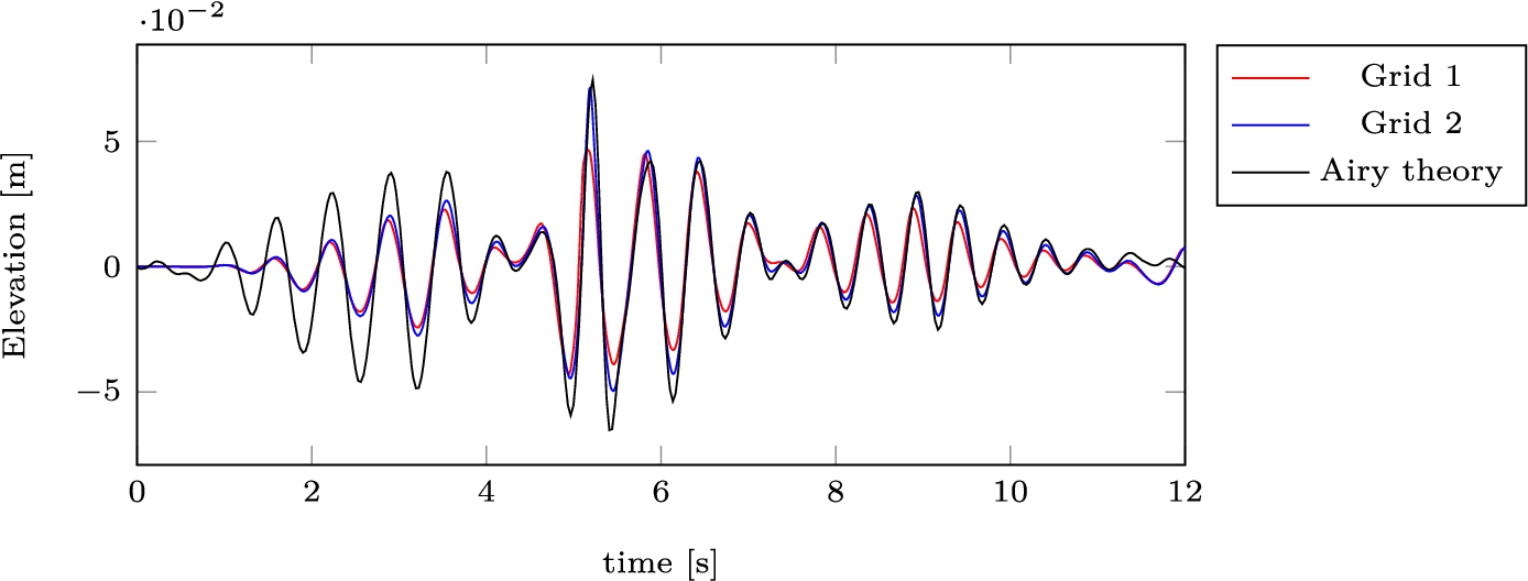
Using only linear Airy theory, the signal of the wave gauge that was fixed to the towing carriage was transformed to its Fourier components to get frequencies, amplitudes and phases. Using the Doppler shifted dispersion relation that accounts for the forward ship speed to get the wave number, the phases were adjusted to account for the distance between the position of the wave gauge and CoG of the ship. Those same Fourier components are used in two ComFLOW simulations, with the open domain boundary at the position of the wave gauge, yielding an output wave signal at the position of CoG. The first ComFLOW simulation, Grid 1, used Δx=0.08 m or 15 cells per shortest wave length. The second ComFLOW simulation, Grid 2, used twice the number of cells per shortest wave length.

The comparison between using only Airy theory and using the ComFLOW simulations with the two grid resolutions is shown in Fig. 9. The differences between 0 and 4 seconds are due to ComFLOW ramping up the signal from 0 to the desired output. The difference in the peak at 5 seconds between the two ComFLOW simulations is because the dispersion errors of especially the shortest wave components are smaller for the finer grid. The differences between linear Airy theory and the ComFLOW simulations for the time larger than 4 s are because ComFLOW includes the nonlinear interactions between wave components.

Because the ComFLOW simulations are expected to be a better representation of what the wave signal at CoG in the experiment would have been, the output of the finer ComFLOW simulation at CoG is converted to its Fourier transform as input for Fastship.

Fig. 9.

Free surface elevation in Fastship and 2D ComFLOW simulations at the position CoG (experiment not available).

The heave and pitch motion found with Fastship for run 42 are shown in Fig. 12, in which they are compared to the experiment. The axis system in Fastship, with the vertical axis downward, is different from the axis system in the experiment, with the vertical axis upward. The pitch rotation in Fastship is positive anti-clockwise, whereas it is positive in clockwise direction in the experiment. It was found after comparing Fastship output to the experiment, however, that the axis system of the ship in Fastship, positive downward, is inconsistent with the axis system of waves in Fastship, positive upward. For that reason, sinkage and trim from a Fastship run without waves were subtracted from the motion signals. The resulting signal was corrected before being recombined with sinkage and trim. The corrected signals are in Fig. 12. The accelerations at CoG are also corrected and visualized in Fig. 13, where they are compared to the experiment. It is found from comparing the Fastship motions and accelerations to the experiment, that the overall behaviour is consistent with the experiment. The magnitude of the vertical acceleration is higher around 5 s and underpredicted in the remainder. The motions are underpredicted over the entire time span.

5.3.ComFLOW

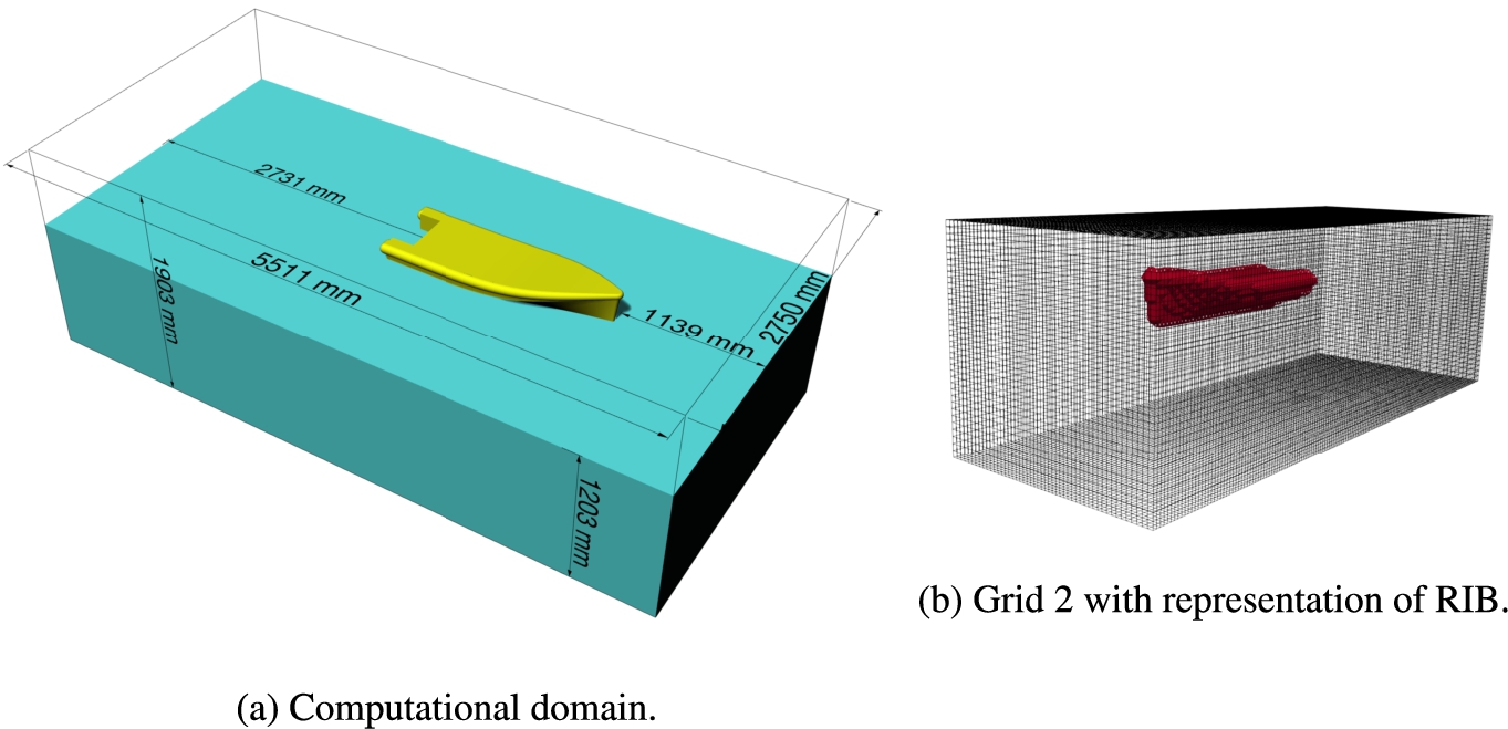
The dimensions of the ComFLOW domain are based on Wellens [26]. Along the line of wave propagation it is advised to make the domain two typical wave lengths larger than the structure in either direction, to keep the wave absorbing boundary conditions away from splashes and wave breaking near the structure and to allow nonlinear wave interaction to take place between the incoming and reflected wave systems. For this simulation, with forward speed of the RIB it was decided to shift the structure one typical wave length closer to the incoming wave boundary for two reasons. The first reason is because the reflected wave system propagating ahead of the RIB was expected to be small. The second reason is because we wanted to keep the stationary wave system behind the RIB as small as possible near the aft boundary so as not to disturb the wave absorbing boundary condition on that side too much. In x-direction, in the direction of wave propagation, the domain extends from −2.2 m to 3.3 m with CoG of the RIB at x=0. In transverse direction, the domain is the same size as the towing tank. In vertical direction, the mean free surface coincides with z=0, with the bottom positioned at z=−1.203 m to match the water depth in the experiment and the top of the domain at z=0.7 m, sufficiently far away not to interfere with the motions of the ship, nor the free surface. The domain is visualized in Fig. 10a.

Fig. 10.

Snapshots of computational domain and grid.

From the 2D wedge simulations, it was found that 8 and 16 cells along the width of the RIB are sufficient to capture the vertical motion behaviour. In longitudinal direction, there are two requirements to the grid spacing. The grid size cannot be too different from the transverse direction to keep the free surface reconstruction algorithm accurate, and the grid size needs to be small enough to keep numerical wave dispersion and numerical wave dissipation sufficiently small. To keep numerical errors small, there need to be approximately 15 cells in the shortest wave length in the spectrum. The minimum grid sizes in the simulations close to CoG of the vessel are Δx,Δy,Δz=0.08,0.08 and 0.09 m, with 1% of stretching in y-direction, and 2% in z-direction. This grid gives us 8 cells along the width of the RIB. We call this grid 1. For comparison, a refined grid 2 was used with cells twice as small. Grid 2, having at least 16 cells along the width of the RIB is visualized in Fig. 10b, , including the RIB reconstruction. Cut-cells are used for the object, giving a good representation for the wedge shaped ship. We are interested in the global motion and therefore not interested in representing boundary layers around the hull that would require a much higher grid resolution. The maximum CFL number allowed for all ComFLOW simulations is 0.85. The maximum time step varied with the variation of the CFL number and never exceeded 0.001 s.

The default boundary conditions in ComFLOW have been discussed in Section 2 above. We have performed calm water runs and runs with irregular incoming waves. In order to perform wave simulations, a Dirichlet boundary condition for the horizontal velocity is imposed at the incoming wave boundary, in combination with the Generating Absorbing Boundary Condition described in Wellens and Borsboom [28]. One advantage of the GABC is that incoming and outgoing wave boundaries can be closer to the object in the domain. The coefficients of the absorbing boundary condition on the incoming and outgoing ends of the domain are a1=0.573, a1=0 and b1=0, making them effectively Sommerfeld boundary conditions tuned to 0.573gh, with g the acceleration of gravity and h the water depth. The horizontal velocity is computed from a sum of Airy wave velocity components, which are ramped up from 0 to the obtained velocity signal over approximately 4 seconds. The frequencies, amplitudes and phases for the wave components come from the Fourier transform of the signal of the wave gauge connected to the towing carriage. The phases are then corrected with the wave number for each component, multiplied by the position of the resistance type wave gauge in the simulation domain, x=−1.858 m. To demonstrate that the wave signal at the position of the wave gauge in ComFLOW is the same as in the experiment, those signals are plotted in Fig. 11. We will focus on the time span between 4 and 9 s, indicated by the grey markers in Fig. 11, because this is the time over which the velocity of the ship is constant.

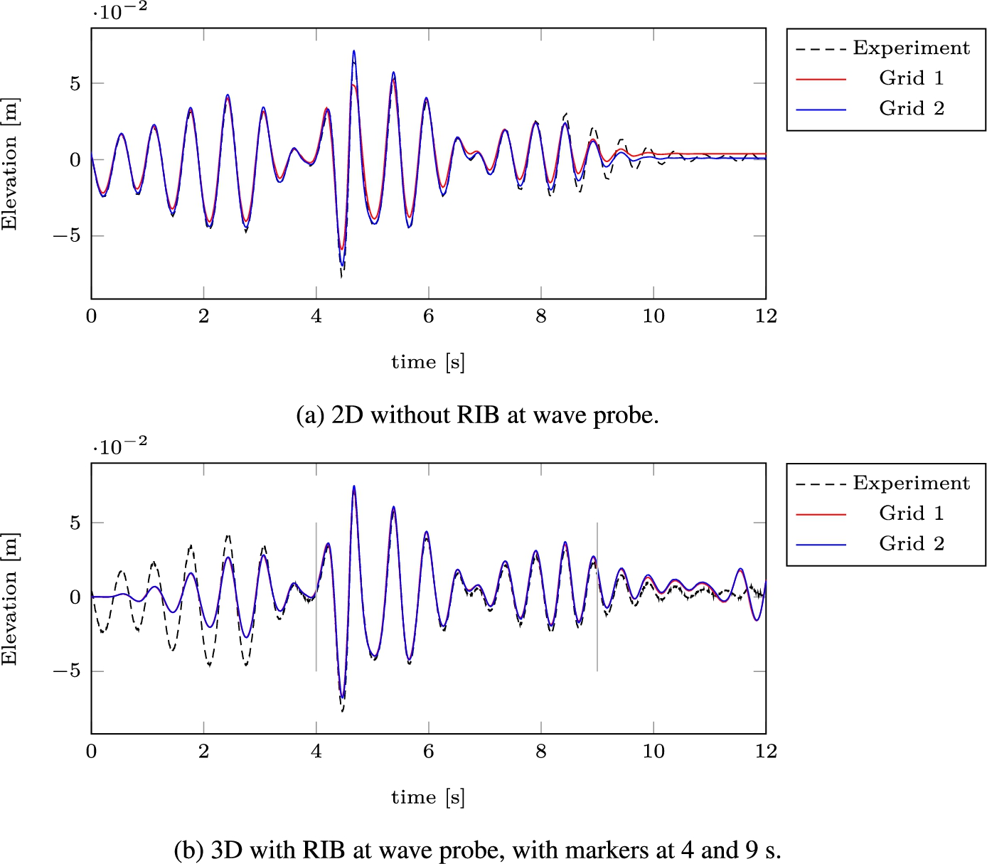
Fig. 11.

Free surface elevation comparison.

5.4.Comparison results: Calm water simulation

Runs in initially calm water were performed at different ship forward velocities in the experiment, in Fastship and in ComFLOW. Table 4 shows the velocities and the sinkage and trim for all methods, together with the Froude number based on the length of the RIB. Trim is in good agreement between ComFLOW and the experiment. Sinkage shows the same trend in ComFLOW and the experiment, but there is a small difference. The ComFLOW runs were performed without a turbulence model. The boundary layer underneath the ship, being dominated by numerical viscosity, is unlikely to have the correct size. This could be an explanation for the difference.

Table 4

Comparison steady values Fastship and ComFLOW with experiment (* indicates a failed run)

	Run nr.	Velocity (m/s)	Sinkage (mm)	Trim (deg)
Experiment	24	1	*	*
Fastship	24	1	2.1	0.89
ComFLOW	24	1	4.9	1.61
Experiment	46	2	22.9	2.44
Fastship	46	2	8.0	4.43
ComFLOW	46	2	19.0	2.63

The trim and sinkage found by Fastship are quite different from the experiment. Specifically for Run 46, the sinkage is nearly three times as small as in the experiment and the trim is nearly two times as high. Here, we must make a note that Fastship was never specifically designed for the velocity range in this article, but for higher forward ship velocities. A specific calibration for the velocity range in this article will likely improve the Fastship results. However, we did not do this because we wanted to remain consistent with the settings used by Keuning et al. [11]. While the difference in sinkage is still under investigation, the difference in trim is most likely due to an incomplete representation of the boxes in the waterline at the stern in Fastship between ordinate 0 and 2 in Fig. 8; lack of restoring moment there can cause an overprediction of trim. Mean sinkage and trim are subtracted from the wave signals in the next section. In Fastship, the unsteady motions (heave, pitch) are treated independently from the steady position (sinkage, trim) and an error in the steady position will not lead to additional errors in the unsteady motions.

5.5.Comparison results: Motion and acceleration in irregular waves

Runs with waves were performed for different significant wave heights, measuring heave, pitch and the accelerations at the CoG. The runs were done for depth Froude numbers of 0.6 and higher and Froude numbers based on length of the RIB as in Table 2. Mean heave and mean pitch were subtracted from the signals and the normalized root mean square (rms) difference between the experiment on the one side, and Fastship and ComFLOW (for two grids) on the other was determined according to

(8)ϵnrms=∑i=1n(yˆ−y)2n·1y¯,

where y¯ is the range between maximum and minimum of the simulation results yˆ. The motions in Run 42, for which the rms difference between the experiment and ComFLOW is about the mean of all rms differences, are given in Table 5, among other runs. It is found that the difference between the experiment and Fastship is consistently larger than between the experiment and ComFLOW (for both grids).

Table 5

Comparison values Fastship and ComFLOW with experiment

Error (–)	Run nr.	Velocity (m/s)	Fastship	ComFLOW 1	ComFLOW 2
ϵnrms,acc [–]	42	2	0.146	0.067	0.107
ϵnrms,heave [–]	42	2	0.198	0.157	0.085
ϵnrms,pitch [–]	42	2	0.211	0.086	0.052
ϵnrms,acc [–]	44	2	0.157	0.071	0.097
ϵnrms,heave [–]	44	2	0.162	0.143	0.117
ϵnrms,pitch [–]	44	2	0.193	0.092	0.073
ϵnrms,acc [–]	48	2	0.167	0.068	0.112
ϵnrms,heave [–]	48	2	0.203	0.145	0.101
ϵnrms,pitch [–]	48	2	0.223	0.080	0.063

Figure 12 shows heave and pitch of the RIB in the ComFLOW simulation of Run 42, where it is compared to Fastship and to the experiment. Note that mean heave and mean pitch for the Fastship and ComFLOW results have been replaced by the mean heave and pitch in the experiment. From these figures we find that heave and pitch in the simulations are of the same order of magnitude as the experiment, but the difference between Fastship and the experiment is larger than the difference between ComFLOW and the experiment. Fastship consistently underestimates the motions with respect to the experiment. In Section 4.4 it was also found that the deceleration of 2D falling wedges is larger than that of the 3D falling wedge. It needs to be investigated whether 2D versus 3D, with Fastship being based on strips of 2D wedges, could be an explanation for the lower motions. Acceleration is never truly computed in ComFLOW and therefore not part of the output. The acceleration at CoG in ComFLOW is found from numerical differentiation of the ship velocities in time in combination with a butterworth filter of order 5 with a normalized cutoff frequency of 1/250. The accelerations at CoG are shown in Fig. 13. From the figure we find that the vertical accelerations in experiment and simulations are of the same order of magnitude. The agreement in acceleration between ComFLOW and the experiment is better than the agreement between Fastship and the experiment. Fastship underestimates the vertical acceleration, except for the peak at the time mark of 5 s. The differences between the results of the different ComFLOW grids are consistent with the differences between results for the wedge, and sufficiently small to trust the results. A visual illustration of the ComFLOW simulation and the experiment for run 42 is shown in Fig. 14.

Fig. 12.

Numerical motion compared with experimental data.

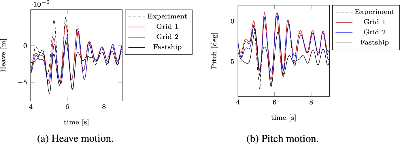
Fig. 13.

Comparison of acceleration with experimental data.

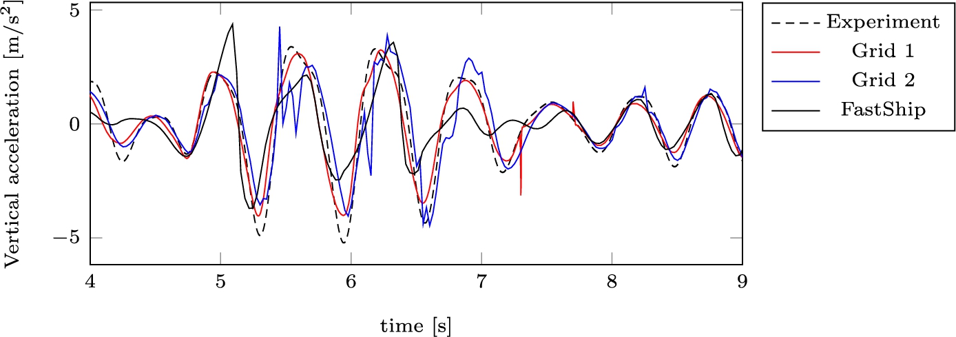
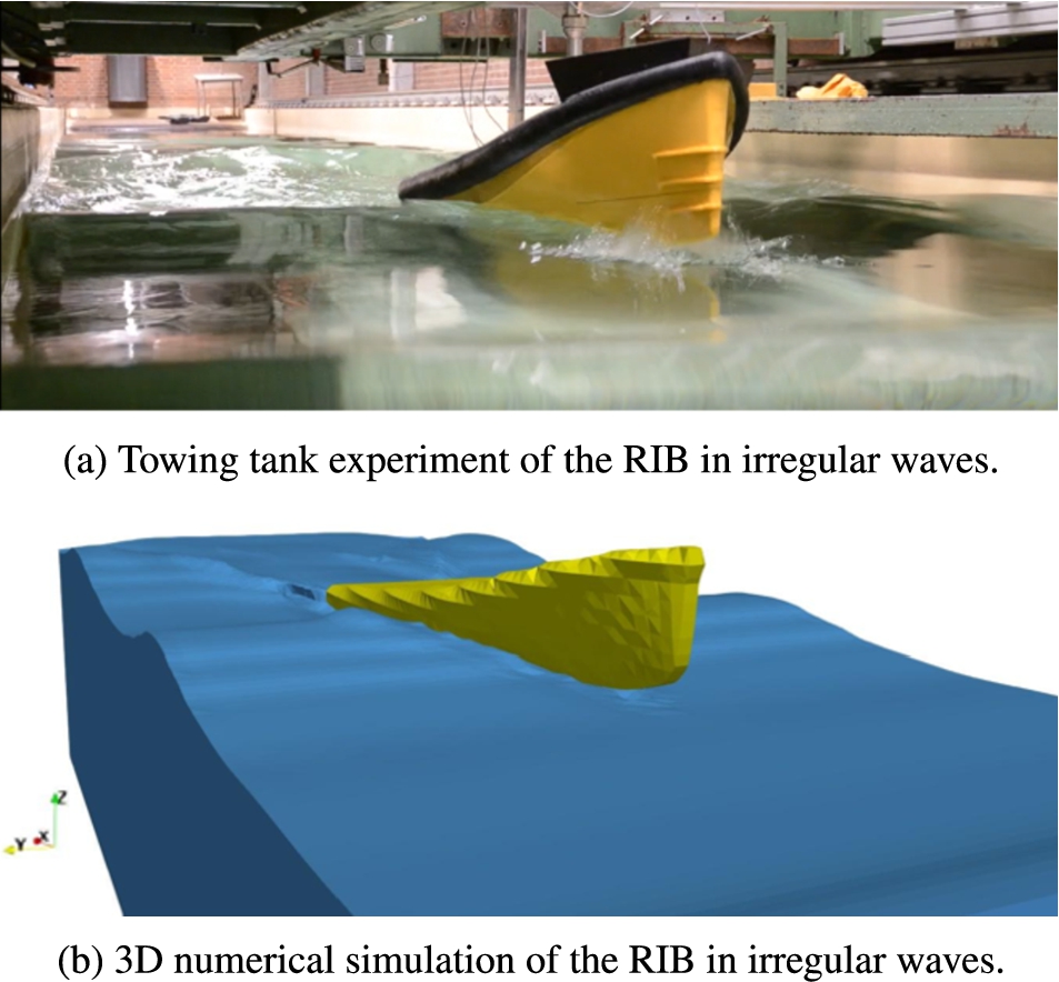
Fig. 14.

Visual comparison of the towing tank experiment and the numerical simulation.

6.Conclusions

This paper is about the vertical accelerations during a bow re-entry of a Rigid Inflatable Boat (RIB) in irregular waves. Its main contribution is the complete deterministic comparison in time of the first-principles numerical method ComFLOW with the results of a self-conducted towing tank experiment in terms of vertical accelerations in irregular waves. The vertical accelerations are also compared with the state-of-the-art strip-theory method Fastship.

The results of the wedge drop test showed that the effect of air on the vertical motion of the wedge is marginal for a 30 degrees deadrise angle, making the one-phase model more suitable to use in terms of computational effort. A minimum of 8 cells along the width of the model is considered appropriate to represent the vertical motion of the wedge and also the RIB in waves.

Using these outcomes, the simulation results with ComFLOW showed an underestimation of the heave and pitch amplitudes with respect to the towing tank experiment. The mean of the rms differences between the experiment and ComFLOW are given in Table 5. According to Table 5, the results with Fastship are found to underestimate the motions more than ComFLOW. The simulated accelerations in ComFLOW are hardly different from the experiment. The vertical acceleration from ComFLOW is closer to the experiment than the acceleration from Fastship with a smaller normalised rms difference with the experiment of at least 33%.

In terms of computational effort, Fastship is faster. Fastship results are finished in mere seconds per run, whereas ComFLOW requires at least 2 hours on a 20-core dedicated machine to complete a run. For ComFLOW, however, no calibration with experiments is required. A model like Fastship will always remain necessary for rapid assessment, but now with ComFLOW we have an additional means to evaluate RIBs in terms of accelerations and to improve models like Fastship.

Acknowledgements

The authors wish to show their appreciation to Peter Poot, Jasper den Ouden, Jennifer Rodrigues Monteiro, Frits Sterk and Pascal Chabot of Delft University of Technology for the preparation of the experiment and support during the execution of the experiment. We would also like to thank Jacco Nollen, Marnix Bockstael, Roos Tiel, Ernst Mulder, Anke Marije Elzinga and Pepijn Heij of the same institute for the contribution to the numerical simulations. Our gratitude goes out to Hugo Verhelst and Reinier Bos for reading the article and giving feedback.

References

[1]	A.G. Avci and B. Barlas, An experimental and numerical study of a high speed planing craft with full-scale validation, Journal of Marine Science and Technology 26: ((2018) ), 617–628.
[2]	R.W. Bos and P.R. Wellens, Fluid–structure interaction between a pendulum and monochromatic waves, Journal of Fluids and Structures 100: ((2021) ), 103191. doi:10.1016/j.jfluidstructs.2020.103191.
[3]	R. Broglia and D. Durante, Accurate prediction of complex free surface flow around a high speed craft using a single-phase level set method, Computational Mechanics 62: ((2018) ), 421–437. doi:10.1007/s00466-017-1505-1.
[4]	G. Bullock, A. Crawford, P. Hewson, M. Walkden and P. Bird, The influence of air and scale on wave impact pressures, Coastal Engineering 42: ((2001) ), 291–312. doi:10.1016/S0378-3839(00)00065-X.
[5]	B. Duz, Wave generation, propagation and absorption in CFD simulations of free surface flows, Ph.D. thesis, Delft University of Technology, 2015.
[6]	O.M. Faltinsen, Hydrodynamics of High-Speed Marine Vehicles, Cambridge University Press, (2005) .
[7]	G. Fekken, Numerical simulation of free-surface flow with moving rigid bodies, Ph.D. thesis, University of Groningen, 2004.
[8]	G. Fekken, A. Veldman and B. Buchner, Simulation of green-water loading using the Navier–Stokes equations, in: Proceedings 7th Intern. Conf. on Numerical Ship Hydrodynamics, Nantes, (1999) .
[9]	T. Fu, K. Brucker, S. Mousaviraad, C. Ikeda, E. Lee, T. O’shea, Z. Wang, F. Stern and C. Judge, An assessment of computational fluid dynamics predictions of the hydrodynamics of high-speed planing craft in calm water and waves, in: 30th Symposium on Naval Hydrodynamics, (2014) , pp. 2–7.
[10]	J. Gerrits, Dynamics of liquid-filled spacecraft: Numerical simulation of coupled solid-liquid dynamics, Ph.D. thesis, University of Groningen, 2001.
[11]	J. Keuning, G. Visch, J. Gelling, W. De Vries Lentsch and G. Burema, Development of a new SAR boat for the Royal Netherlands Sea Rescue Institution, in: 11th Int. Conference on Fast Sea Transportation, FAST 2011, Honolulu, Hawaii, USA, (2011) .
[12]	J.A. Keuning, Nonlinear behaviour of fast monohulls in head waves, Ph.D. thesis, Delft University of Technology, 1996.
[13]	K. Kleefsman, G. Fekken, A. Veldman, B. Iwanowski and B. Buchner, A volume-of-fluid based simulation method for wave impact problems, Journal of computational physics 206: ((2005) ), 363–393. doi:10.1016/j.jcp.2004.12.007.
[14]	C. Lai, A.W. Troesch et al., Modeling issues related to the hydrodynamics of three-dimensional steady planing, Journal of Ship research 39: ((1995) ), 1–24. doi:10.5957/jsr.1995.39.1.1.
[15]	S.G. Lewis, D.A. Hudson, S.R. Turnock, J.I. Blake, R. Shenoi et al., Predicting motions of high speed RIBs: A comparison of non-linear strip theory with experiments, in: HIPER 06: 5th International Conference on High-Performance Marine Vehicles, Australian Maritime College, (2006) , p. 210.
[16]	J. Marges, FRISC kent eigen kracht niet, 2018, https://magazines.defensie.nl/allehens/2018/01/00_frisc.
[17]	S.M. Mousaviraad, Z. Wang and F. Stern, URANS studies of hydrodynamic performance and slamming loads on high-speed planing hulls in calm water and waves for deep and shallow conditions, Applied Ocean Research 51: ((2015) ), 222–240. doi:10.1016/j.apor.2015.04.007.
[18]	S. Muzaferija, A two-fluid Navier–Stokes solver to simulate water entry, in: Proceedings of 22nd Symposium on Naval Architecture, 1999, National Academy Press, (1999) , pp. 638–651.
[19]	R. Peterson, E. Pierce, B. Price and C. Bass, Shock mitigation for the human on high speed craft: Development of an impact injury design rule, Technical Report, Naval Surface Warfare Center Panama City (FL), 2004.
[20]	A.A. Rijkens, Proactive control of fast ships: Improving the seakeeping behaviour in head waves, Ph.D. thesis, Delft University of Technology, 2016.
[21]	S. Tavakoli, S. Najafi, E. Amini and A. Dashtimanesh, Performance of high-speed planing hulls accelerating from rest under the action of a surface piercing propeller and an outboard engine, Applied Ocean Research 77: ((2018) ), 45–60. doi:10.1016/j.apor.2018.05.004.
[22]	M. Van Der Eijk and P.R. Wellens, A compressible two-phase flow model for pressure oscillations in air entrapments following green water impact events on ships, International Shipbuilding Progress 66: ((2020) ), 315–343. doi:10.3233/ISP-200278.
[23]	H.A. Van der Vorst, Bi-CGSTAB: A fast and smoothly converging variant of Bi-CG for the solution of nonsymmetric linear systems, SIAM Journal on scientific and Statistical Computing 13: ((1992) ), 631–644. doi:10.1137/0913035.
[24]	A.F. Van Deyzen, Improving the operability of planing monohulls using proactive control: From idea to proof of concept, Ph.D. thesis, Delft University of Technology, 2014.
[25]	S. Wang, Y. Su, X. Zhang and J. Yang, RANSE simulation of high-speed planning craft in regular waves, Journal of Marine Science and Application 11: ((2012) ), 447–452. doi:10.1007/s11804-012-1154-x.
[26]	P.R. Wellens, Wave simulation in truncated domains for offshore applications, Ph.D. thesis, Delft University of Technology, 2012.
[27]	P.R. Wellens, Experimental data for a Rigid Inflatable Boat (RIB) undergoing slamming in irregular waves, 4TU.ResearchData, 2020. doi:10.4121/13078601.
[28]	P.R. Wellens and M. Borsboom, A generating and absorbing boundary condition for dispersive waves in detailed simulations of free-surface flow interaction with marine structures, Computers & Fluids 200: ((2020) ), 104387. doi:10.1016/j.compfluid.2019.104387.
[29]	R. Wemmenhove, Numerical simulation of two-phase flow in offshore environments, University of Groningen, 2008.
[30]	P. Xu and P. Wellens, Effects of static loads on the nonlinear vibration of circular plates, Journal of Sound and Vibration 504: ((2021) ), 116111. doi:10.1016/j.jsv.2021.116111.
[31]	D.L. Youngs, An interface tracking method for a 3D Eulerian hydrodynamics code, Atomic Weapons Research Establishment (AWRE) Technical Report 44, 1984.
[32]	Z.M. Yuan, X. Zhang, C.Y. Ji, L. Jia, H. Wang and A. Incecik, Side wall effects on ship model testing in a towing tank, Ocean Engineering 147: ((2018) ), 447–457. doi:10.1016/j.oceaneng.2017.10.042.
[33]	R. Zhao, A simplified nonlinear analysis of a high-speed planing craft in calm water, in: Proceedings of FAST’97, Sydney, (1997) .
[34]	R. Zhao, O. Faltinsen and J. Aarsnes, Water entry of arbitrary two-dimensional sections with and without flow separation, in: Proceedings of the 21st Symposium on Naval Hydrodynamics, (1996) , pp. 408–423.