A control strategy for combined DP station keeping and active roll reduction

2.1.Thrust allocation

Rudaa et al. [17] propose to use thruster pairs to counteract the wave induced roll moment. When the thruster pairs are fixed and pointing in opposing direction, this yields three main advantages:

Fig. 1.

Schematic thruster pair configuration for roll reduction purposes. Dashed lines indicate a thruster pair.

The thruster pairs work in counterphase to achieve maximum roll reduction. The thrusters are also used for station keeping. In beam waves, the wave forces that need to be counteracted by the control model are mainly in the sway direction. Since thruster T2 and T4, see Fig. 1, are already pointing in the direction of the incoming wave loads, these thrusters are used for station keeping in the sway direction.

The yaw motion is controlled by the bow thruster, since this thruster has a long yaw moment arm and is not used for roll reduction purposes. Therefore, the complete thruster capacity can be used to control the yaw motion.

Since all thrusters are aligned in the sway direction, compensation of environmental forces in the surge direction is not possible. To solve this, the azimuth angle of the thrusters used for surge control are controlled by an azimuth controller. Thruster T3 is used for compensation of positive surge forces and thruster T5 is used to compensate negative surge forces. A schematic visualization of the thrusters used for station keeping in sway, surge and yaw direction is given in Fig. 2.

Fig. 2.

Thruster configuration for station keeping in the horizontal plane (left: sway, middle:surge and right: yaw motion). Dashed lines indicate which thruster (pair) controls which motion.

2.2.Control system structure

The vessel motions are controlled by a hierarchical control system. The system consists of high-level motion controllers and low-level shaft speed (τs, τDP and τϕ, where ϕ indicates the roll motion) and azimuth angle controllers (τazi). The control structure is visualized in Fig. 3

Fig. 3.

Schematic 3DP control system structure.

A shaft speed controller is implemented to control the shaft speed of the dynamic thruster model. The high-level motion controllers are merged by superimposing the shaft speed controller command for DP with the shaft speed controller command for active roll reduction. The principle hereof is visualized in Fig. 4.

Fig. 4.

Schematic visualization of high-level motion control merging principle.

As illustrated in Fig. 4, merging the roll reduction controller and the DP controller results in a decrease of the roll reduction capacity by increasing the minimum number of shaft revolutions per minute (RPM).

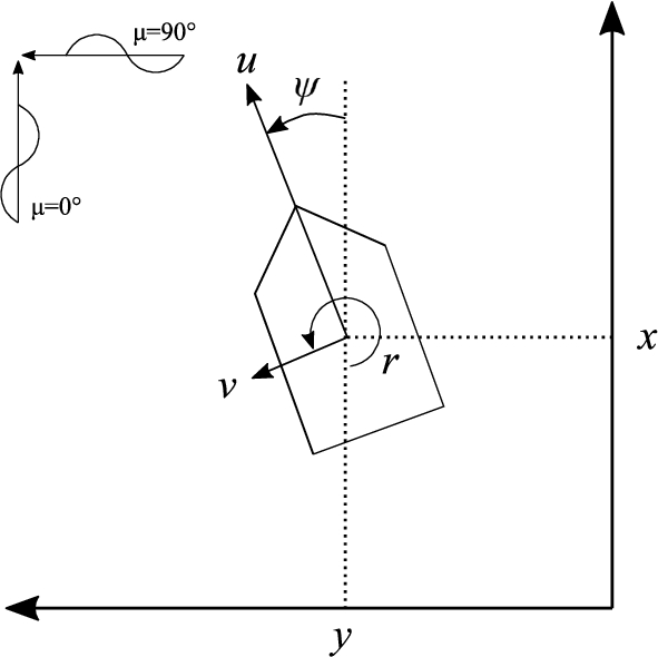
3.1.Kinematics

The horizontal vessel motions surge, sway and yaw as calculated by the model are based on a body-fixed reference frame [u,v,r] and a earth-fixed reference frame [x,y,ψ]. The vessel motions, velocities and accelerations are calculated in the body-fixed frame and are subsequently translated to the earth-fixed frame by using the rotation matrix:

Fig. 5.

Definition of reference frames and environmental load direction μ.

3.2.Time domain model

In order to calculate the vessel’s (linearized) motion response when subjected to (non-linear) forces and moments induced by the thrusters and the environment, a 6 degree of freedom time domain model is used. The time domain model is based on Cummins [3]:

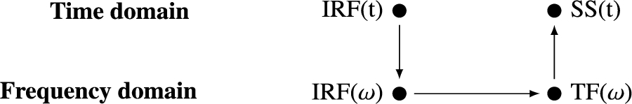
There exist different methods to evaluate the convolution term in the Cummins’ equation, see Armesto et al. [1]. A state-space method is used, due to its favourable computational performance. It is possible to approximate the convolution operation in Cummins’ equation by a state-space model:

Fig. 6.

Schematic visualization of the strategy used to obtain a time domain state-space representation.

The impulse response function is calculated numerically in the time domain for every motion and coupling term according to Journée [8]:

Subsequently, the impulse response function is transferred to the frequency domain according to Duarte and Sarmento [5]:

3.3.Viscous roll damping

Viscous effects and energy dissipation are neglected when diffraction analysis based on linear potential theory is used. Since the motions of a ship other than roll are dominated by potential damping, diffraction analysis is, in general, sufficiently accurate at predicting the motion response. For the roll motion, however, viscous effects are dominant. Vortex shedding at the bilge induces damping of the ship.

According to Chakrabarti [2], the viscous roll damping term can be expressed by a third-order polynomial:

In the time domain model it is possible to incorporate a quadratic damping term Bvisc|η4˙|η4˙, with Bvisc a tuning parameter that is found by iterating the time domain roll motion Response Amplitude Operator (RAO) until it matches the frequency domain roll motion RAO for a unit wave amplitude. The time domain model with the viscous damping term included in the (4,4) position of Bvisc is now expressed by:

3.4.Environmental forces

The vessel motions are induced by waves, wind and current. The wave force consists of a first- and a second-order component. The first-order wave force (indicated by superscript (1)) is expressed in the time domain as:

The low-frequency and mean wave drift force (indicated by superscript (2)) in irregular waves are calculated in the time domain according to Newman [13] by:

A similar approach is used to calculate the forces and moment due to the current:

3.5.Dynamic thruster model

To achieve thruster induced roll reduction, the thrusters need to counteract the first-order roll moment. The dynamic response of the thrusters is therefore important to model. Since fixed-pitch propellers are assumed, the thruster dynamics are governed by the inertia of the thruster system, propeller torque demand, torque produced by the electrical motor and shaft friction. This can be formulated according the simulation model proposed by Smogeli [20]:

The hydrodynamic pitch angle β is defined by:

The shaft friction term is defined by [20]:

Smogeli [20] acknowledges that an added inertia term due to the hydrodynamic forces in phase with the propeller rotational acceleration exists, but chooses to neglect it. An involved method based on lifting lines for the hydrodynamic properties of open water propellors is available in Krüger and Abels [11]. An empirical estimate of the inertia term of open water propellors can be obtained from MacPherson et al. [12] and Schwanecke [18]. In reality, DP propellors are ducted and below the ship. Methods or data for those circumstances are – to our knowledge – not readily available. Not knowing how close either method is to our specific situation, we chose to base our inertia term on the lesser involved empirical methods of MacPherson et al. [12] and Schwanecke [18] as follows.

In the latter two references, the added rotational inertia term of the entrained water is defined by:

Since both empirical models are based on model test results carried out with different propeller types, the average of the model results is used as a representative value for the inertia term.

The thrusters experience oscillating inflow velocities as a result of the roll motion of the vessel. Therefore, the four-quadrant model as developed by Oosterveld [15] is used to calculate the thruster torque demand and thrust production:

The roll moment of the thrusters is calculated by multiplying the produced thrust in the sway direction with the thruster moment arm. The thruster moment arm is defined as the vertical distance from the centre of the thruster to the centre of gravity (CoG) of the vessel.

3.6.3DP control strategy

The high level motion controller is a combination of a conventional DP controller and roll controller:

The thruster shaft speed is controlled by a PI controller as proposed by Smogeli [20]:

In beam waves, the wave forces acting on the vessel in the surge direction are negligible. However, wind and current can induce significant forces in the surge direction when their direction differs from the wave direction. To increase the station keeping capability of the vessel, the azimuth angle of the thrusters allocated to control the surge motion is controlled by a proportional controller:

3.7.Controller tuning

Tuning of the controllers is important to ensure stable vessel behaviour. A first estimate of the proportional, integral and derivative gains of the high-level DP controller τDP is obtained by the rules of thumb proposed by Serraris [19].

The first estimates of the proportional and integral gain terms of the low-level shaft speed controller τs are based on parameter estimates as presented in the work of Smogeli [20]. The controller gains of both controllers are tuned manually until the desired stable system behaviour was obtained.

The high-level anti-roll controller and the low-level azimuth angle controller are tuned by conducting systematic numerical experiments. In this way both controllers are tuned such that roll reduction is at maximum.

3.8.DP model

The station keeping performance of the control model is compared to a conventional DP control system to analyze the effect of active roll reduction onto the DP footprint. The conventional DP system consists of a Kalman filter, PID controller and an allocation algorithm [19]. The coefficients of the Kalman filter and the PID controller of the conventional DP system are kept the same as in our proposed roll reduction control model to ensure equal comparison.

4.1.Vessel particulars

The performance of the control model is analyzed by applying the 3DP model to a barge-shaped offshore construction vessel. The vessel particulars are given in Table 2.

In Table 2, L is the length of the vessel, B the width, T is the draft, ∇ the displacement and Tϕ is the natural roll period. Barge-shaped vessels are particularly sensitive to roll motions due to their large B/T-ratio.

The vessel is equipped with 5 thrusters in total, of which 4 azimuthing thrusters and 1 bow thruster. The thruster lay-out is given in Fig. 1. The DP control point is located in the vessel’s CoG. The DP setpoint is defined as [0,0,0].

The thruster particulars are given in Table 3.

4.2.Environmental conditions

The vessel is subjected to several environmental conditions to assess the performance of the control model for roll reduction together with station keeping. The simulated environmental conditions are given in Table 4.

It is assumed that the wind and current forces act co-linearly with the waves (μ=90∘). The wave peak period is chosen equal to the natural roll frequency of the vessel. A JONSWAP spectrum with peak enhancement factor γ=3.3 is used to calculate the wave loads. The parameter Mt/Menv represents a dimensionless ratio, in which Mt and Menv represent the maximum roll moment induced by the thrusters and the mean of the absolute first-order wave roll moment. The total simulation time is set to 0.5 hour, since critical situation during typical operations take less time than that.

4.3.Allocation

The thrusters that are used for station keeping and roll reduction are indicated by the allocation matrices H1 and H2. The allocation vector H1 is used to indicate which thrusters are used to control the surge, sway and yaw motions:

5.1.Time domain model validation

The motion response amplitude operators (RAOs) for quartering regular waves as calculated by the time domain model, without a viscous roll damping term included, are compared with frequency domain RAOs to confirm the validity of the state-space modelling approach, see Fig. 7.

Fig. 7.

Comparison of calculated RAOs by both frequency and time domain model (μ=45∘).

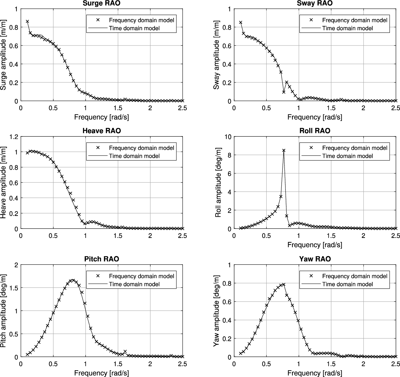
From Fig. 7, we find that both models are in agreement, because the state-space representation of the convolution term yields the same results as the frequency domain model results.

5.2.Viscous roll damping

The time domain model parameter Bvisc is obtained by tuning the time domain model roll motion RAO in beam waves with the frequency domain model RAO. The resulting RAOs are given in Fig. 8.

Fig. 8.

Comparison of roll RAO calculated by both frequency and time domain model, including viscous roll damping term (μ=90∘).

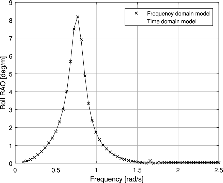
It can be confirmed from the RAO visualized in Fig. 8 that the time domain tuning method results in a similar roll motion RAO for both models. By iterating, the quadratic tuning parameter in the time domain model was determined to be 6% of the critical roll damping (based on moment of inertia and added moment of inertia).

One should be aware of the fact that this roll motion RAO only matches for a unit wave amplitude. When a lower wave amplitude is used, the time domain model will underestimate the viscous damping in comparison with the frequency domain model due to the inclusion of a quadratic viscous damping term. The opposite applies when a higher wave amplitude is applied. Since the maximum simulated significant wave height is 1 m, this approach will result in less viscous damping compared to frequency domain analysis. This is considered to be a conservative approach, since the thrusters will have to counteract a bigger roll moment and will therefore reach their saturation limit more early compared to the frequency domain model.

5.3.Tuning

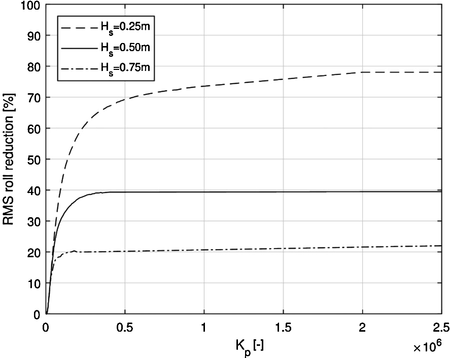
Systematic numerical simulations for the different environmental conditions were carried out to tune the anti-roll and azimuth controllers. The relative RMS roll reduction is calculated for different controller gains. The result of the anti-roll controller tuning procedure is given in Fig. 9. Figure 9 indicates that the roll RMS reduction percentage converges towards the higher values for Kp of the roll reduction controller.

Fig. 9.

Tuning of the controller gain for roll reduction: roll RMS reduction percentage for different values Kp of the anti-roll controller (Tp=8.5 s).

To tune the azimuth controller, the relative RMS roll reduction is calculated for different directions of the environmental load. The tuning coefficients are increased systemically per direction. The results are given in Fig. 10

Fig. 10.

Tuning of the azimuth controller: roll RMS reduction percentage for different Kp values of the azimuth controller and the direction of the environmental load (Hs=0.5 m, Tp=8.5 s).

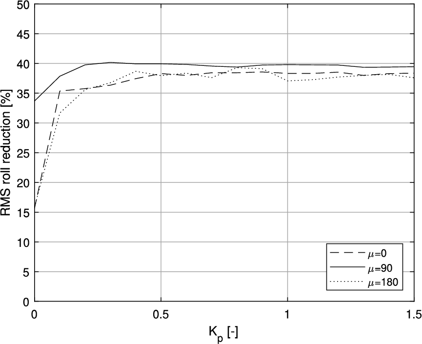
From Fig. 10, it can be observed that the maximum roll reduction for all investigated directions of the environmental load occurs at a value of Kp=0.9 for the azimuth controller gain.

The tuning coefficients of the DP controller in the 3DP control strategy and the Kalman filter tuning parameters Q and R are given in Table 5.

The controller coefficients as used in the 3DP control model for the roll controller, azimuth controller and shaft speed controllers are summarized in Table 6. Note that a different ship would require the described procedure to be executed again to obtain new numbers for adequate performance.

5.4.Roll reduction

To analyze the performance of the proposed roll reduction control model, the roll angle amplitudes are compared to the roll angle amplitudes obtained when roll is not actively reduced in the conventional DP model. Both models are subjected to equal environmental forces. A snapshot of the vessel roll angles as a function of time for both models is visualized in Fig. 11.

Fig. 11.

Snapshot of the roll angles time trace for simulation case 1.

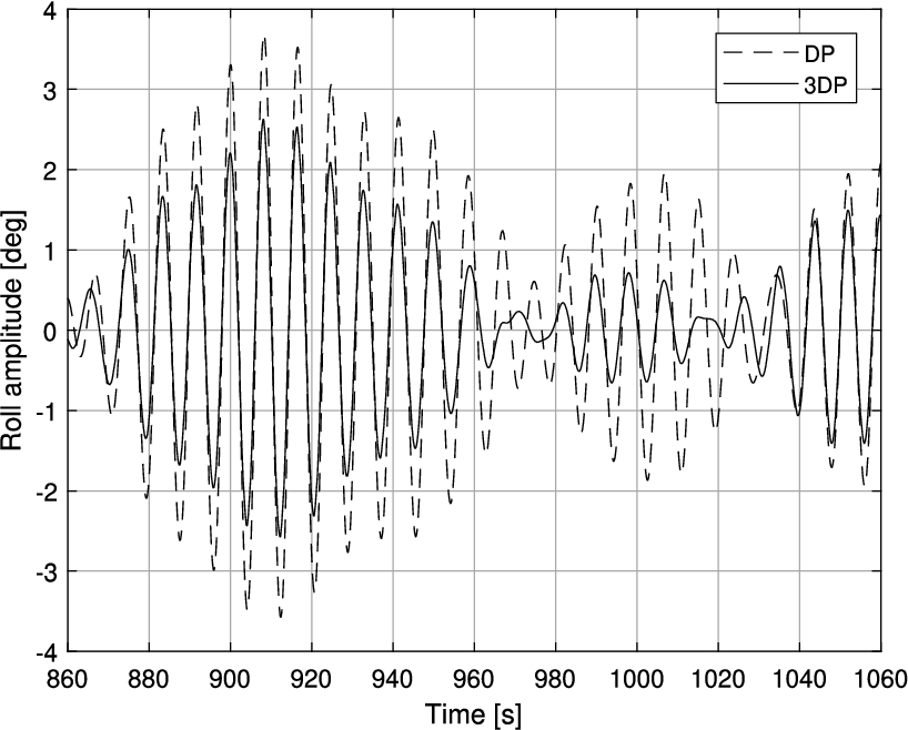
As can observed in Fig. 11, the roll reduction varies in magnitude every period. As a way to visualize the realized roll reduction, the roll angle amplitudes are translated to a normal distribution. The results are given in Fig. 12.

Fig. 12.

Normal distribution of roll for simulation case 1, 2 and 3 (from top to bottom).

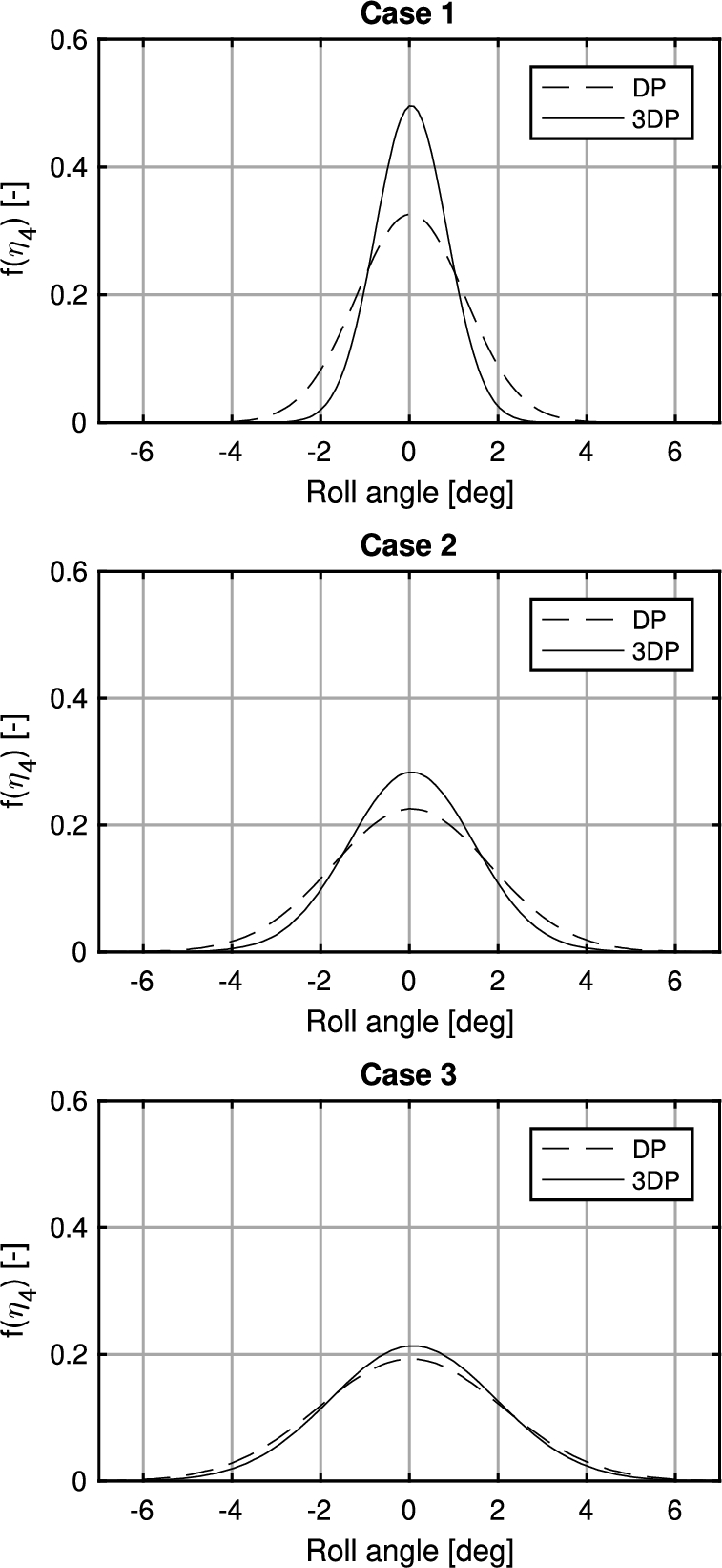
Shown in Fig. 12 is that the effect of active roll reduction is most significant for simulation case 1. The variance of the roll amplitude decreases and the probability density of the mean amplitude of 0∘ increases when the 3DP model is applied. The effect of active roll reduction decreases when the significant wave height increases. To also quantify the results, the root mean square (RMS), maximum value and absolute mean of the roll angle time traces are calculated, see Table 7.

Table 7 confirms the observed behavior in Fig. 12. The roll reduction percentages decrease when the significant wave height increases. This is because the roll moment realized by the thrusters is not able to compensate for the first-order wave roll moment as the significant wave height increases. The ratio between the thruster roll moment and first-order wave roll moment Mt/Menv can be seen in Table 4. The roll reduction also decreases in higher sea states because the thrusters require more power for DP station keeping purposes when the significant wave height increases.

5.5.Station keeping

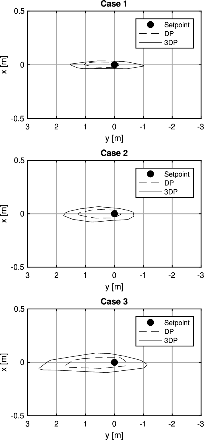
The vessel’s station keeping performance can be assessed by analyzing the DP footprint of the vessel. The DP footprint visualizes the maximum excursions of the vessel in the horizontal earth-fixed reference frame with respect to the DP setpoint. To analyze the performance of the proposed control model, the DP footprint of both the proposed model and the conventional DP model is visualized in Fig. 13. Figure 13 shows that the increase of the 3DP footprint is small compared to the conventional DP footprint in Case 1 and Case 2. For Case 3, with the highest significant wave height, the footprint in y-direction is increased by 1 m, which is 1% of the vessel length.

Fig. 13.

DP footprint of proposed control model and DP model for simulation case 1, 2 and 3 (from top to bottom).

The yaw motion behavior is interesting. Thrust variations result in significant yaw moments which the vessel’s DP controller has to counteract. A normal distribution has been used to visualize the yaw station keeping performance of the vessel, see Fig. 14.

Fig. 14.

Normal distribution of yaw angles of proposed control model and DP model for simulation case 1, 2 and 3 (from top to bottom).

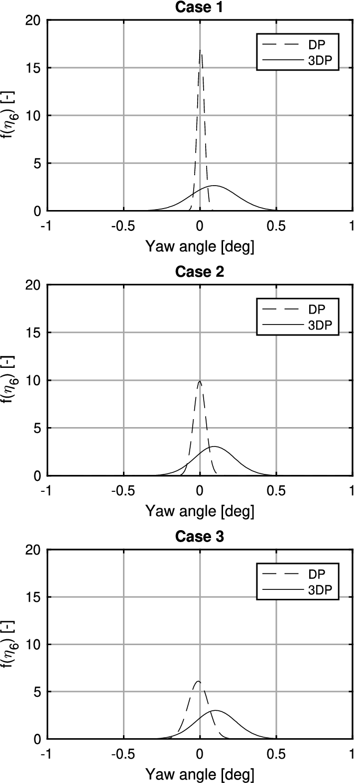
From Fig. 14 we find that the DP model has the highest probability density at a yaw angle of 0∘. This is as expected, since the DP model yaw angle setpoint is 0∘. Figure 14 also shows that the variance increases proportionally to the significant wave height. This is due to the fact that the vessel motions increase for higher environmental loads.

The 3DP model results show that the highest probability density is shifted slightly towards a yaw angle of 0.1∘. The yaw moments induced by the thrusters in the 3DP model are significantly higher compared to the DP model. The Ki coefficient of the DP controller in the 3DP model should have been increased to remove the yaw offset. However, for a fair comparison, it was decided to use the same controller coefficients in both the DP and the 3DP model.

The plots show that the probability density function remains nearly constant in larger significant wave heights. This is because the yaw moments induced by the thrusters are significantly larger than the yaw moments resulting from waves, current and wind.

The yaw angle variance of the 3DP model is also bigger compared to the DP model. This is explained by the oscillating yaw moments induced by the thrusters during active roll reduction. The maximum increase of the yaw angle variance is 0.7∘, which is considered acceptable.

5.6.Station keeping capability

Next to the vessel DP footprint, also the station keeping capability is of interest. The station keeping capability is defined by the limiting current speeds at which the vessel is still able to maintain position. It is give by the positioning limits in DNV-GL [4] for DP capability level 3. Those limits are a maximum of 5 meter excursion and a maximum of ±3∘ yaw angle excursion.

In our investigation, the current velocity is increased per environmental condition until the vessel exceeds the positioning limits. The highest current velocities at which the vessel was still able to maintain position are visualized in Fig. 15.

Fig. 15.

Limiting current speeds per environmental direction for simulation case 1, 2 and 3.

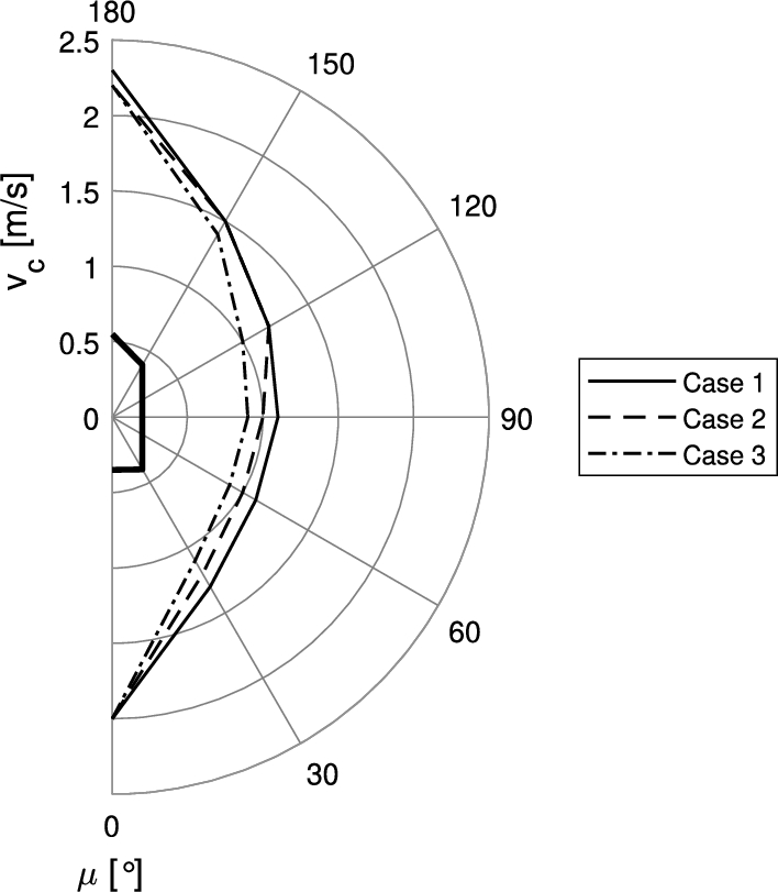
From Fig. 15, we find that the vessel is able to maintain position in current velocities up to 2.3 m/s in head seas and 2.0 m/s following seas. In beam seas the station keeping capability is limited by a current velocity of 1.1 m/s, 1.0 m/s and 0.9 m/s for simulation case 1, 2 and case 3, respectively.

5.7.Power consumption

The cost of active roll reduction is expressed in terms of increased power consumption. The sum of the power consumption of every thruster is calculated to obtain the total power consumption of the control system over time. The mean of the total power consumption of the 3DP and the DP control model is calculated and is expressed in a percentage of the total installed thruster power. The results are given in Fig. 16.

Fig. 16.

Mean power consumption percentage of total installed DP power for case 1, 2 and 3.

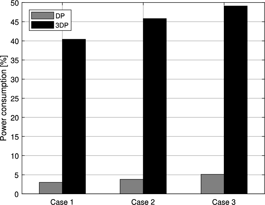
As expected, Fig. 16 indicates that the power consumption of the 3DP control system is higher compared to the DP system, and becomes higher for higher sea states. It was also to be expected that the power consumption of the thrusters is around 50% of the total installed thruster power, since the thrusters are working 50% of their time at high thrust levels to counteract the roll moment. The power consumption of the 3DP model is around a factor 10 higher than the conventional DP model during brief critical moments in operations.

References

[1] | J.A. Armesto, R. Guanche, F. del Jesus, A. Iturrioz and I.J. Losada, Comparative analysis of the methods to compute the radiation term in Cummins’ equation, Ocean Engineering and Marine Energy 1: ((2015) ), 377–393. doi:10.1007/s40722-015-0027-1. |
[2] | S. Chakrabarti, Empirical calculation of roll damping for ships and barges, Ocean Engineering 28: ((2001) ), 915–932. doi:10.1016/S0029-8018(00)00036-6. |
[3] | W.E. Cummins, The impulse response function and ship motions, in: Symposium Ship Theory, Hamburg, Germany, (1962) . |
[4] | DNV-GL, ST-0111 Assessment of station keeping capability of dynamic positioning vessels, DNV-GL Standard, 2016. |
[5] | T. Duarte and A. Sarmento, State-space realization of the wave-radiation force within FAST, in: 32th ASME Conference on Ocean, Offshore and Arctic Engineering OMAE2013, (2013) . |
[6] | Y. Himeno, Prediction of ship roll damping – state of the art, University of Michigan, 1981. |
[7] | Y. Ikeda, T. Fujiwara and T. Katayama, Roll damping of a sharp-cornered barge and roll control by a new-type stabilizer, in: Proceedings of the Third International Offshore and Polar Engineering Conference, Singapore, (1993) . |
[8] | J.M.J. Journée, Hydromechanic coefficients for calculating time domain motions of cutter suction dredgers by Cummins equation, TU Delft Report 968, 1993. |
[9] | D. Jürgens and M. Palm, Voith Schneider propeller – an efficient propulsion system for DP controlled vessels, in: Dynamic Positioning Conference, (2009) . |
[10] | P. Koschorrek et al., Dynamic Positioning with active roll reduction using Voith Schneider propeller, in: 10th IFAC Conference on Manoeuvring and Control of Marine Craft, (2015) . |
[11] | S. Krüger and W. Abels, Hydrodynamic damping and added mass of modern screw propellers, in: International Conference on Offshore Mechanics and Arctic Engineering, Vol. 7B: Ocean Engineering, (2017) . doi:10.1115/OMAE2017-61470. |
[12] | D.M. MacPherson, V.R. Puleo and M.B. Packard, Estimation of entrained water added mass properties for vibration analysis, in: SNAME New England Section, (2007) . |
[13] | J.N. Newman, Marine Hydrodynamics, MIT Press, Cambridge MA, (1970) . |
[14] | U. Nienhuis, Simulation of low-frequency motions of dynamically positioned offshore structures, in: Royal Institution of Naval Architects Spring Meeting, London, (1986) . |
[15] | M.W.C. Oosterveld, Wake Adapted ducted propellers, PhD thesis, Delft University of Technology, Delft, 1970. |
[16] | J.A. Pinkster, Low frequency second order wave exciting forces on floating structures, PhD thesis, Delft University of Technology, Delft, 1980. |
[17] | S.E. Rudaa, S. Steen and V. Hassani, Use of tunnel and azimuthing thruster for roll damping of ships, in: 10th IFAC Conference on Control Applications in Marine Systems, (2016) . |
[18] | H. Schwanecke, Gedanken zur Frage der Hydrodynamisch Erregten Schwingungen des Propellers und der Wellenleitung, Jahrbuch der Schiffbauteschnischen Gesellschaft, Vol. 57: , (1963) . |
[19] | J.J. Serraris, Time domain analysis for DP simulations, in: 28th ASME Conference on Ocean, Offshore and Arctic Engineering OMAE2009, (2009) . |
[20] | Ø.N. Smogeli, Control of marine propellers, PhD thesis, NTNU, Trondheim, 2006. |
[21] | A.J. Sørensen and J.P. Strand, Positioning of small-waterplane-area marine constructions with roll and pitch damping, Control Engineering Practice 8: ((2000) ), 205–213. doi:10.1016/S0967-0661(99)00155-0. |
[22] | J. Wichers, S. Bultema and R. Matten, Hydrodynamic research on and optimizing dynamic positioning system of a deep water drilling vessel, in: Offshore Technology Conference, (1996) . |
[23] | S. Xu et al., Mitigating roll-pitch motion by a novel controller in dynamic positioning system for marine vessels, Ships and offshore structures 12: ((2017) ), 1136–1144. doi:10.1080/17445302.2017.1316905. |