
CFD, potential flow and system-based simulations of fully appended free running 5415M in calm water and waves
Abstract
The seakeeping ability of ships is one of the aspects that needs to be assessed during the design phase of ships. Traditionally, potential flow calculations and model tests are employed to investigate whether the ship performs according to specified criteria. With the increase of computational power nowadays, advanced computational tools such as Computational Fluid Dynamics (CFD) become within reach of application during the assessment of ship designs. In the present paper, a detailed validation study of several computational methods for ship dynamics is presented. These methods range from low-fidelity system-based methods, to potential flow methods, to high-fidelity CFD tools. The ability of the methods to predict motions in calm water as well as in waves is investigated. In calm water, the roll decay behavior of a fully appended self-propelled free running 5415M model is investigated first. Subsequently, forced roll motions simulated by oscillating the rudders or stabilizer fins are studied. Lastly, the paper discusses comparisons between experiments and simulations in waves with varying levels of complexity, i.e. regular head waves, regular beam waves and bi-chromatic waves.
The predictions for all methods are validated with an extensive experimental data set for ship motions and loads on appendages such as rudders, fins and bilge keels. Comparisons between the different methods and with the experiments are made for the relevant motions and the high fidelity CFD results are used to explain some of the complex physics. The course keeping and seakeeping of the model, the reduction rate of the roll motion, the effectiveness of the fin stabilizers as roll reduction device and the interaction of the roll motion with other motions are investigated as well. The paper shows that only high-fidelity CFD is able to accurately predict all the relevant physics during roll decay, forced oscillation and sailing in waves.
1.Introduction
The simulation of ship course keeping and seakeeping has mostly been studied using potential flow (PF) and system-based (SB) methods and more recently computational fluid dynamics (CFD). The assessment of the capability of these approaches is required to employ them in the ship design process. In the last two years, NATO AVT-161 and 216 groups under the NATO Science and Technology Organization were formed to assess the capability of the prediction methods for ship seakeeping and maneuvering in deep and shallow water. This paper is part of the work concentrating on the prediction capability in calm water, regular and bi-chromatic waves for deep water conditions which is conducted for 5415M surface combatant. It is a first step in a collaborative effort towards the numerical prediction of ship motions in irregular waves. The benchmark data for 5415M seakeeping were provided by MARIN. The collected data consisted of the 6DOF motions of the ship and forces and moments acting on the appendages such as bilge keels, rudders and stabilizer fins for different tests. The tests included roll decay and forced roll (by means of stabilizer fins or rudders) in calm water and seakeeping in regular, bi-chromatic and irregular waves. The measured data provided a unique opportunity to investigate the prediction capability of SB, PF and CFD methods for complicated 6DOF ship motions and forces and moments on the appendages.
In the past, SB models have been applied extensively to estimate ship maneuvering capabilities. The prediction capability of SB methods is strongly dependent on empirical formulae or the inputs for maneuvering coefficients, the degree of freedom of the model and the setup of the mathematical models to include the waves, the rudder and the propulsion forces. Therefore, SB predictions for different SB tools are different and they often show only qualitative results. Toxopeus and Lee [34] used several simulation tools to predict the maneuverability of different ship hulls including KVLCCs, 5415M and KCS. It was shown that the difference between SB predictions and the experiments depended strongly on the range of application of each prediction tool: MPP (originally made for full-block ships) provided good results for the KVLCCs, FreSim (for naval ships) for the 5415M and SurSim with slender body method (for cruise ships, ferries, motor yachts) for the KCS.
Unlike SB models, the PF methods employ strip theory, lifting line/surface or panel methods to compute directly the forces and moments used to predict the 6DOF motions of a ship. However, empirical corrections to account for viscous effects are required (see Yen et al. [37] and Toxopeus and Lee [34]). An extensive benchmark study of state-of-the-art seakeeping prediction tools was presented by Bunnik et al. [4]. In this study, 11 different codes (9 PF codes and 2 CFD codes, of which one was ISIS-CFD) were used to calculate motions of ships in a seaway. Generally, it was found that most of the PF codes used in the study produce good results. When the motions are moderate and in the absence of large viscous effects (flow separation, frictional damping) or wave breaking, the benefit of using CFD instead of the best PF methods was found to be small.
In the last few years, CFD simulations have advanced from captive to free running 6DOF conditions with controllers and moving appendages and propellers, which provides the opportunity to study maneuvering, capsize and course keeping in calm water and waves. One of the first applications was from Sato et al. [28] who conducted a study in which their viscous-flow solver was coupled to the equations motions of the ship. The instantaneous forces on the hull were calculated using CFD, while the forces due to the propeller and rudder were calculated using empirical formulae based on the MMG model. With their model, they performed zig-zag maneuvers for two Very Large Crude Carrier (VLCC) variants. Comparison with the experiments showed reasonable quantitative agreement. The results of a workshop regarding simulation of maneuvers of several benchmark ships were presented at SIMMAN 2008 for calm water condition (Stern et al. [30]). The workshop provided a successful quantitative assessment of the maneuvering prediction capabilities for typical tanker, container, and combatant hulls. Sadat-Hosseini et al. [21,22,24], Carrica et al. [6] and Mousaviraad et al. [18] presented maneuvering in calm water and regular waves for surface combatants (ONR tumblehome and 5415M) and a surface effect ship (SES). For surface combatants, the results showed good predictions of maneuvering in calm water with an error of 2–7%D for various trajectory characteristics. The simulations in waves showed the same order of error for most of the trajectory characteristics. For SES, the simulations were conducted in both deep and shallow water and in both calm water and waves. It was shown that shallow water increases transfer and tactical diameter in turning maneuvers and reduces the overshoot angles for zigzag. Additionally, it was shown that the wave effect could be significant on the maneuver of the ship in shallow water.
The most commonly used propeller model in the previous maneuvering studies is the axisymmetric body force method which is specified in a non-iterative manner such that the ship wake on the body force is neglected. Sadat-Hosseini et al. [25,27] studied propeller modeling effect on maneuvering of a tanker with a single propeller, using the fully discretized rotating propeller and two body force propeller models including non-iterative axisymmetric and interactive Yamasaki body force propeller models. The simulations with fully discretized rotating propeller provided the lowest error among different propeller models, The trajectory characteristics were predicted with an error of 8–10%D for various maneuvers. The errors were up to three times larger for the non-iterative axisymmetric body force propeller model and 50% larger for the interactive Yamasaki body force propeller model. Other research has focused on improving the SB mathematical model by using CFD with system identification (SI) methods for both calm water (Sadat-Hosseini et al. [21,22,25]; Araki et al. [1]) and following waves (Araki et al. [2]). They used two system identification methods including extended Kalman filter (EKF) and constrained least square (CLS). The results in calm water showed the average system based prediction errors for maneuvering simulations drop from 16% to 8% by using the maneuvering coefficients and rudder forces found from CFD free running instead of those from captive experiments. Also, the system based results in waves were significantly improved by tuning the maneuvering coefficients and wave forces in the mathematical model using CFD outputs. Such an approach was also followed by Toxopeus [33] in which RANS calculations were used to derive coefficients for an SB model. The results of subsequent maneuvering simulations were compared with model experiments, demonstrating a large improvement compared to the simulations with the original coefficients derived from empirical formulae.
The objective of the present paper is to assess the capabilities of CFD, PF, and SB methods for course keeping in calm water and regular and bi-chromatic waves for 5415M as a benchmark test case for AVT-161. The behavior of the model in irregular waves is dealt with in Sadat-Hosseini et al. [23]. Herein, the results are investigated with consideration to the mathematical model of 6DOF ship motions similar to the analysis performed for parametric rolling and broaching by Sadat-Hosseini et al. [22,26]. The 6DOF mathematical model is based on third-order Taylor series approximation of forces and moments about an equilibrium position. The model explains the influence of the coupling of different modes of motions on the forces/moments which can assist analyzing the CFD predictions. Also, a detailed validation study is performed for forces and moments on the appendages including rudders, fins and bilge keels and the high fidelity results are used to explain some of the complex physics.
CFD computations are performed using the CFDShip-Iowa and ISIS-CFD codes. PF simulations are performed with Fredyn, SWAN and LAMP. The SB roll decay and forced roll predictions are carried out by using the SurSim and FreSim.
2.5415M test case
2.1.Hull form
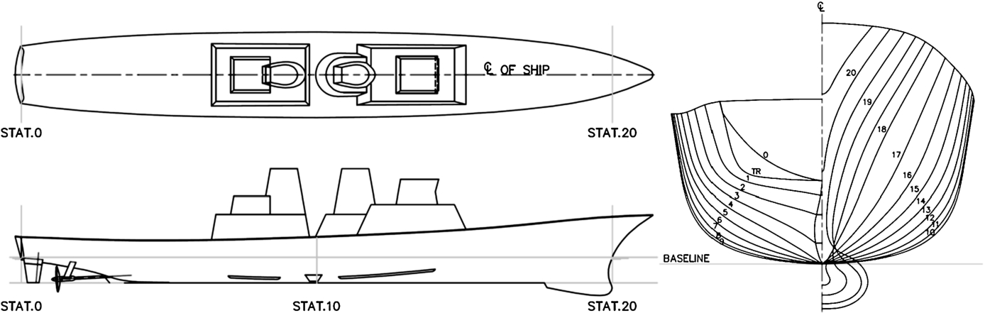
Free running experiments in calm water and waves were conducted for 5415M. The 5415M model is a geosim of the DTMB 5415 ship model, but with modified appendages and skeg. Main particulars and body plan are shown in Table 1 and Fig. 1, respectively. The model was manufactured of wood and appended with skeg, twin split bilge keels, roll stabilizer fins, twin rudders and rudder seats slanted outwards, shafts and struts, and twin propellers. The rudder was of the spade type. The lateral area of the rudders was 2 × 15.4 m2 i.e. 2 × 1.8% of the lateral area of the vessel, L × T. The propellers were fixed pitch type with direction of rotation inward over top. The stabilizer fins were of the non-retractable, low aspect ratio type. The scale ratio of the model was 35.48.
Table 1
DTMB5415M main particulars
| Length: L | 142.0m | Natural period of roll | 11.50s |
| Breadth: B | 19.06m | Roll radii of gyration: | 0.4B |
| Draft: T | 6.15m | Pitch and yaw radius of gyration: | 0.25 L |
| Volume of displacement: ∇ | 8432 m3 | Propeller diameter: | 6.15m |
| Transverse metacentric height: GM | 1.95m | Pitch at 0.7R: P0.7R | 5.32m |
| Block coefficient: | 0.507 | Expanded blade area ratio: AE/A0 | 0.58 |
| Rudder area | 15.4m2 | Fin stabilizer area | 6 m2 |
Fig. 1.
DTMB 5415M geometry and body plan.
2.2.Test setup
All experiments were carried out in the MARIN Seakeeping and Maneuvering Basin. The tests were performed with the ship model free running and the propeller rate of revolutions adjusted to the self-propulsion point of the model for the approach speed of the maneuver. During the test, the wave elevation, ship motions, ship accelerations, rudder and fin angles and propellers revolutions were measured. Also, propeller torque and thrust and loads on bilge keels, rudders and fins were recorded. The wave elevations were measured in front of the vessel and beside the vessel at mid-ship using resistance-type wave probes and used to represent the wave elevation at center of gravity. The ship motions were recorded through optical tracking system. The ship accelerations were measured at three locations on the model using accelerometer. Several Potentio-meters were employed to measure rudder and fin angles. Strain gauge transducers were used to measure loads on the propellers, rudders, and fins. For loads on bilge keels, one-component force transducers were utilized. More details of the test setup can be found in Toxopeus et al. [35].
The coordinate system is ship-fixed located at centre of gravity, with x pointing toward the bow, y to portside and z upward. The roll (ϕ) is positive for starboard down, the pitch (θ) is positive for bow down and the yaw angle (ψ) is positive for bow turned to portside. The forces and moments are positive for X-force forwards, Y-force to portside, Z-force upward, K-moment pushing starboard into the water, M-moment pushing the bow into the water and N-moment pushing the bow to portside. The rudder angle (δ) is positive for a rotation with the trailing edge to portside and the stabilizer fin angles (
2.3.Test conditions
A subset of the full experimental program with the self-propelled free model appended with passive, active, or no fin stabilizers was selected for the present study. The selection comprises roll decay and forced roll tests and tests in regular waves and in bi-chromatic waves. The conditions for different tests in calm water and waves are summarized in Table 2.
Table 2
EFD, CFD, PF, and SB test cases in calm water and waves
| Test Id. | Test Type | Fin Type | SelectedTest Conditions | Codes |
| 1.1 | Free roll decay | Without Fin | SB: SurSim, FreSim PF: Fredyn, LAMP, SWAN2 CFD: CFDShip-Iowa, ISIS-CFD | |
| 1.2 | Passive Fin | SB: SurSim, FreSim PF: Fredyn, LAMP, SWAN2 CFD: CFDShip-Iowa, ISIS-CFD | ||
| 1.3 | Active Fin | SB: SurSim, FreSim PF: Fredyn, LAMP CFD: CFDShip-Iowa | ||
| 2.1 | Forced roll due to rudders | Passive Fin | Amplitude = 15 deg Period = 11.42 s (full scale) | SB: SurSim, FreSim PF: Fredyn, LAMP CFD: CFDShip-Iowa |
| 2.2 | Active Fin | Amplitude = 15 deg Period = 11.42 s (full scale) | SB: SurSim, FreSim PF: Fredyn CFD: CFDShip-Iowa | |
| 2.3 | Forced roll due to Fin | Forced Fin | Amplitude = 25 deg Period = 11.42 s (full scale) | SB: SurSim, FreSim PF: Fredyn, LAMP CFD: CFDShip-Iowa |
| 3.1 | Seakeeping in regular waves | Active Fin | PF: Fredyn, LAMP CFD: CFDShip-Iowa | |
| 4.1 | Seakeeping in bi-chromatic waves | Active Fin | μ: 300 deg | PF: Fredyn, LAMP CFD: CFDShip-Iowa |
Herein, the cases are selected based on careful study of the test results for validation of the computations. All selected tests were conducted at a speed corresponding to
3.CFD method
3.1.CFDShip-Iowa 4.5
CFDShip-Iowa is an overset, block structured CFD solver using non-orthogonal curvilinear coordinate system for arbitrary moving control volumes. Turbulence models include blended
3.1.1.Computational domain and grids
For cases in calm water, the domain is in cylinder shape with the radius of 4.5 L extending from
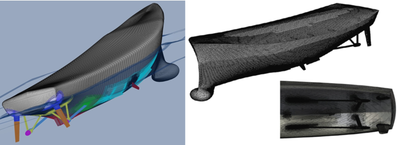
The computational grids are overset, with independent grids for the hull, appendages, refinement and background, and then assembled to generate the total grid. The grids for the hull (boundary layer) are generated with a hyperbolic grid generator using a double-O topology, one each for the starboard and the portside. The same grid topology was used for each rudder and fin to describe their geometry extending out of the hull. The grids are independent and capable to simulate the dynamic rudders and fins. The skeg uses the same grid topology but overset the boundary layer grids. An O topology was used for struts, shafts, and rudder seats. An H-type grid was used for the twin bilge keels, oversetting the boundary layer grids. Since no wall function is used in this study, the first grid point away from all the solid surfaces was selected to be 10−6 m on model scale to capture the details of the flow. For calm water, the background is built using an O-type grid topology to impose far field boundary conditions with an H-type refinement block closer to the ship. For waves, a Cartesian H-type grid topology was used for the background. The total number of grid points is 6.3–7.0M for calm water and 18.6 M for waves, decomposed into respectively 72 and 181 partitions for parallel processing. Details of the grids are shown in Fig. 2.
Fig. 2.
Overset grid system and instantaneous view of the free surface for CFDShip-Iowa (left) and unstructured grid system for ISIS-CFD (right).
3.1.2.Case setup
The experimental conditions are followed as closely as possible in the simulations. In all cases, experimental data are used to impose the initial displacement, velocity, and acceleration. Mimicking the experimental procedures, all cases are run with constant propeller RPM, obtained by two self-propulsion simulations at the corresponding Froude number for the two cases with the ship without and with fins. During the self-propulsion simulations, the ship was only free to surge, heave and pitch while all 6DOF motions are predicted for the other cases. The predicted RPM was 107.8 in full scale for the ship without fin, 1.4% higher than the average of the measured RPM. For the ship with fins, the predicted RPM increased to 113.2, which is 4% higher than the measured one. PID type feedback controllers are used for roll and heading for cases with active fins or rudders. The roll controller produces the angle for the stabilizer fins using the same controller as in the experiment to put the ship back at upright position. The heading controller acts on the rudder attempting to steer the ship to the desired heading. Since the actual coefficients for the heading controller were not recorded during the experiments, a PD controller was employed with P and D estimated from fitting
For the calm water simulation, the time step was set to 0.005 L/V. For the course keeping simulations, 100 time steps per encounter wave period were used. All simulations were conducted using the blended
3.2.ISIS-CFD
ISIS-CFD, developed by the CFD group of the LHEEA laboratory and available as a part of the FINE™/Marine computing suite, is an incompressible unsteady Reynolds-averaged Navier Stokes (URANS) method. The solver is based on the finite volume method to build the spatial discretization of the transport equations. The unstructured discretization is face-based, which means that cells with an arbitrary number of arbitrarily shaped faces are accepted. A detailed description of the solver is given in e.g. Duvigneau and Visonneau [8]. The velocity field is obtained from the momentum conservation equations and the pressure is obtained through the resolution of the discrete pressure equation obtained by combining the discretized mass and momentum conservation equations. In the case of turbulent flows, transport equations for the variables in the turbulence model are added to the discretization. Free-surface flow is simulated with a multi-phase flow approach: the water surface is captured with a conservation equation for the volume fraction of water, discretized with specific compressive discretization schemes discussed in Queutey and Visonneau [20]. The method features sophisticated turbulence models: apart from the classical two-equation
3.2.1.Computational domain and grids
The computational domain extends from
3.2.2.Case setup
The roll decay tests with no fins or passive fins are investigated. Firstly, an initial simulation with a ship free to move in trim and sinkage with no roll angle is carried out. For this simulation, the actuator disk theory is applied, where the thrust is balanced by the drag of the ship. The thrust is applied as body forces in the area of the propeller disc. With this approach, RPM information is not available. At the start of the roll decay simulations, the initial roll angle is applied. The flow around the ship is computed by imposing the surge motion while all other modes of motion are free. Moreover, the rudder action due to the autopilot is ignored in these computations, which may introduce some differences when comparing to the experiments or other computations.
The turbulence mode used is the Explicit Algebraic Reynolds Stress Model (EARSM) based on
4.PF method
4.1.FREDYN
Fredyn is developed by the Cooperative Research Navies (CRNAV) group. Its fundamentals are discussed in De Kat and Paulling [7]. The version considered in this paper is Fredyn version 10.3. Fredyn is a program dedicated to simulate the motions of high-speed semi-displacement ships in severe conditions. The program is intended to be used in the initial design stage when model test data are not available.
The mathematical model consists of a non-linear strip theory approach, where linear (wave radiation and diffraction) and non-linear (Froude–Krylov, including buoyancy) potential flow forces are combined with viscous forces (propeller, bilge keel, rudder and fin forces, hull lift and drag, roll damping, wind loads and etc.). These viscous force contributions are of a nonlinear nature and based on (semi)empirical models. In the present work, the viscous forces are based on the default Fredyn model. The roll damping is based on an adapted method for fast displacement ships (FDS).
A recent application of Fredyn for the 5415M hull form in calm water and waves can be found in Carette and Van Walree [5] and Quadvlieg et al. [19]. Validation of amongst others roll damping predictions or motions in waves with Fredyn can be found in Boonstra et al. [3] and Levadou and Gaillarde [15]. The maneuvering prediction capability of Fredyn was validated by Toxopeus and Lee [34].
The hull form (sectional data) and the particulars of the propeller, bilge keels, rudders and stabilizer fins as described in Section 2.1 were used as input to the program. The bare hull resistance curve was estimated using a modified version of the Holtrop and Mennen method [10]. This method also provides estimates of the propeller wake fraction and thrust deduction fraction. The propeller thrust curve was obtained from open water tests with the model propeller. Other than the use of the propeller open water tests and estimation of the resistance curve, wake fraction and thrust deduction fraction, all coefficients were based on the default values calculated by Fredyn. No additional tuning of the empirical coefficients based on model test data was conducted. The rudder seats were modeled as additional fixed rudders.
During the cases with the rudders steered by autopilot, the coefficients are determined from least-square fitting of the experimental rudder angle signal, see Section 2.3. However, for simplification of the setup, the sway gain coefficient A was ignored. This means that deviations in the y position between the simulations and experiments can occur.
In Fredyn, the RPM of the propellers needs to be specified. In the present work, the RPM from the experiments was used as input. Due to a different balance of resistance and propeller thrust, this may result in a different speed during the simulation.
4.2.SWAN
SWAN2 2002 [31] is a 3D time-domain panel code developed at MIT. Details can be found in Sclavounos [29] and Kring et al. [13]. The software implements a fully 3D approach based on the distribution of Rankine sources over the wetted hull and the free surface. The linear free-surface condition is satisfied, while it has the capability of taking into account the non-linear Froude–Krylov and hydrostatic forces. This option however, was not activated in the present work.
A sensitivity analysis was conducted in order to define a suitable extent of the free surface grid in the longitudinal and lateral directions, as well as the respective number of panels fitted on the wetted surface of the vessel in both directions. The number of desired hull sheet nodes in a direction parallel to the X-axis is 30. The respective number of nodes on a direction perpendicular to X-axis is 8. The panel mesh extends on the free surface 0.5 L upstream, 1.5 L downstream and 1.0 L to the sides. A total of 2300 panels were fitted on the hull form and the free surface.
A time step of 0.05 sec has been used in the calculations. The simulated time history was 300 sec. The code can handle only passive fins, using the actual flow direction to compute the lift on the fin. The rudders are also handled as fins. Furthermore, in the use of SWAN2 an iterative procedure was added to converge to the actual dynamic draft and trim of the vessel at each speed. That pair of draft and trim was subsequently used in the unsteady calculations. In general, the linearity assumption and the fact that viscous roll damping is not taken into account reduces the reliability of the predictions in very high dynamic responses.
4.3.LAMP
LAMP (Large Amplitude Motions Program) is a 3D time-domain dynamic panel code. Forces due to viscous flow effects and other external forces such as hull lift, propulsors, rudders, etc. are modeled using other computation methods or with empirical or semi-empirical formulas. These forces are calculated at each time step and added to the forces from LAMP’s solution of the wave-body hydrodynamics to comprise the right-hand side of a general 6-DOF equation of motions for predicting ship motions. Calm water maneuvering is a special application of the general methodology, without incident wave but retaining the wave-body interactions related to forward speed and ship motions. For a ship maneuvering in waves, either body linear or nonlinear hydrodynamic problems can be solved. The body nonlinear approach, which considers the effects of the ship’s vertical motion relative to the calm water or incident wave, is usually used for the hydrostatic and Froude–Krylov wave forces. Details of the mathematical formulation, numerical implementation and application of LAMP for nonlinear seakeeping or maneuvering problems can be found in e.g. Yen et al. [36,37] and Lin et al. [16,17].
A sensitivity study was carried out to determine the computation domain and grid size. To get stable and converged results, 1388 hydrodynamic body panels were used on the wetted portion of the hull and skeg and 2208 panels were used on a local portion of the free surface. The free surface domain extends from 1 L upstream and 1 L downstream in the longitudinal direction, and extends 1.5 L to starboard and to port side of the ship’s centerline.
The procedure to derive LAMP’s maneuvering forces coefficients was developed and validated for the participation in the SIMMAN 2008 Workshop and is described in Yen et al. [37]. The PMM tests for the workshop were performed at MARIN using an appended model with the propeller rotating at the model self-propulsion point. LAMP’s hull lift model and higher-order damping coefficients were adjusted to fit the measured forces and moments from the PMM test. The bilge keels, rudder, and stabilizing fins were modeled as low aspect ratio lifting surfaces and adjusted to match the measured forces from the PMM tests. The lift of the skeg was modeled as an additional low aspect ratio lifting surface. The open-water propeller thrust curve, wake fraction and thrust deduction, and the velocity increment on rudder inflow due to propeller wash were also modeled from descriptions and data in the test report.
The 6DOF time-domain simulations were carried out for each of the test cases. The LAMP simulations were done at model scale and then converted to full scale for presentation. The propeller RPM for each run was set to achieve the initial, calm-water speed from the experiment and was held constant for the simulation. LAMP’s autopilot, which implements a slightly different algorithm than the autopilot in the experiment, uses the experimental values of P, D, and A, but does not include the rudder bias (
5.SB method
5.1.SurSim and FreSim
SurSim and FreSim are basically the same programs, but with different implementations of the hull forces and rudder/fin forces. All other aspects are modeled using shared libraries. SurSim is dedicated to the simulation of the maneuverability of mainly twin-screw ferries, cruise ships and motor yachts, while FreSim is used for high-speed semi-displacement ships. Both codes model the motions of the ship in four degrees of freedom. SurSim and FreSim do not contain wave modeling and therefore they cannot be applied to study the course keeping of ships in waves. The programs are of the modular type, i.e. forces on each component of the ship are modeled separately. Both models utilize cross flow drag coefficients (see e.g. Hooft [11]) to model non-linear effects in the forces and moments on the ship. The linear maneuvering coefficients are estimated using the slender body method described by Toxopeus [32]. More information about SurSim and FreSim and their validation can be found in Toxopeus and Lee [34]. For maneuvering predictions, FreSim is mostly applicable to slender naval ships, while SurSim is mostly applicable to ships of moderate L/B ratio and moderate block coefficients.
In SurSim and FreSim rudders and fins are modeled as lifting surfaces, treating fins as “rudders” without propeller in front of them. The forces and moments generated by the lifting surfaces are all added in the output files and therefore the forces generated by the rudders cannot be separated from the forces generated by the fins during post-processing and plotting of the results. In this paper, based on the type of test, it was decided to attribute the full loads generated by all lifting surfaces as rudder loads, or as fin loads. In some cases in which both the rudders and the fins generate large forces, disagreement with the loads found during the experiments or with the results from other methods can be expected. Furthermore, bilge keel forces are included in the hull forces and cannot be analyzed separately.
For the setup of the cases (roll decay and forced oscillation) identical input parameters were used for SurSim, FreSim and Fredyn, except for the setting of the propeller RPM. In SurSim and FreSim, the RPM was determined by the program while in Fredyn the RPM value was taken from the measurements. See Section 4.1 for more details of the setup.
6.Presentation and discussion of the results
6.1.Data analysis method
For roll decay cases, the roll damping coefficients are derived based on Himeno Method (Himeno [9]) to study the effects of the stabilizer fins. In this method, it is assumed that the roll motion can be described by the following 1DOF equation:
Here
For forced roll in calm water and cases with waves, the mean, n-th harmonic amplitude and phase of any motion are determined from time histories using Fourier decomposition. In this article, the first harmonic amplitude
The damping coefficients for roll decay in calm water and harmonics for forced roll in calm water and wave cases are compared with EFD data and the comparison error E between the data D and the simulation value S is reported as
All results presented in this article are converted to full scale values using Froude scaling.
6.2.Roll decay in calm water
Table 3 and Fig. 3 show the results for the roll damping cases. During the tests, the model is given an initial roll angle, which subsequently damps quickly such that the roll amplitude decreases to less than a degree in four cycles. Without fins, the damped roll period is about
Table 3
The period and damping coefficients for roll decay
| Type | Parameters | EFD | CFDShipIowa (E%D) | ISIS-CFD (E%D) | Fredyn (E%D) | LAMP (E%D) | Swan2 (E%D) | FreSim (E%D) | SurSim (E%D) |
| No fins | Tϕd (s) | 11.1 | 11.2 | 11.9 | 11.7 | 11.4 | 12.2 | 12.3 | 11.6 |
| (−0.9) | (−7.2) | (−5.4) | (−2.7) | (−9.9) | (−10.8) | (−4.5) | |||
| α (MNms/rad) | 68.1 | 61.1 | 40.7 | 59.9 | 75.4 | 52.5 | 71.1 | 58.8 | |
| (10.3) | (40.2) | (12.0) | (−10.7) | (22.9) | (−4.4) | (13.7) | |||
| β (MNms2/rad2) | 4.28 | 1.65 | 6.64 | 2.41 | 1.17 | 0.62 | 3.54 | 4.70 | |
| (61.4) | (−55.1) | (43.7) | (72.7) | (85.5) | (17.3) | (−9.8) | |||
| Passive fins | Tϕd (s) | 11.3 | 11.3 | 11.9 | 11.7 | 11.5 | 12.2 | 12.5 | 11.7 |
| (0.0) | (−5.3) | (−3.5) | (−1.8) | (−8.0) | (−10.6) | (−3.5) | |||
| α (MNms/rad) | 69.0 | 65.9 | 45.0 | 74.9 | 96.3 | 56.1 | 80.3 | 67.8 | |
| (4.5) | (34.8) | (−8.6) | (−39.6) | (18.7) | (−16.4) | (1.7) | |||
| β (MNms2/rad2) | 14.4 | 16.1 | 12.9 | −0.003 | −3.1 | 0.49 | 4.3 | 4.9 | |
| (−11.8) | (10.4) | (100) | (121) | (96.6) | (70.1) | (66.0) | |||
| Active fins | Tϕd (s) | 12.2 | 12.4 | - | 11.5 | 11.7 | - | 12.8 | 12.0 |
| (−1.6) | (5.7) | (−4.1) | (−4.9) | (1.6) | |||||
| α (MNms/rad) | 202.4 | 89.3 | - | 151.2 | 147.4 | - | 128.6 | 95.0 | |
| (55.9) | (25.3) | (27.2) | (36.5) | (53.1) | |||||
| β (MNms2/rad2) | 20.8 | 22.4 | - | −19.8 | 3.7 | - | 7.1 | 19.1 | |
| (−7.7) | (195) | (82.2) | (65.9) | (8.2) |
Fig. 3.
Roll decay: Without fins (top), passive fins (middle), active fins (bottom).
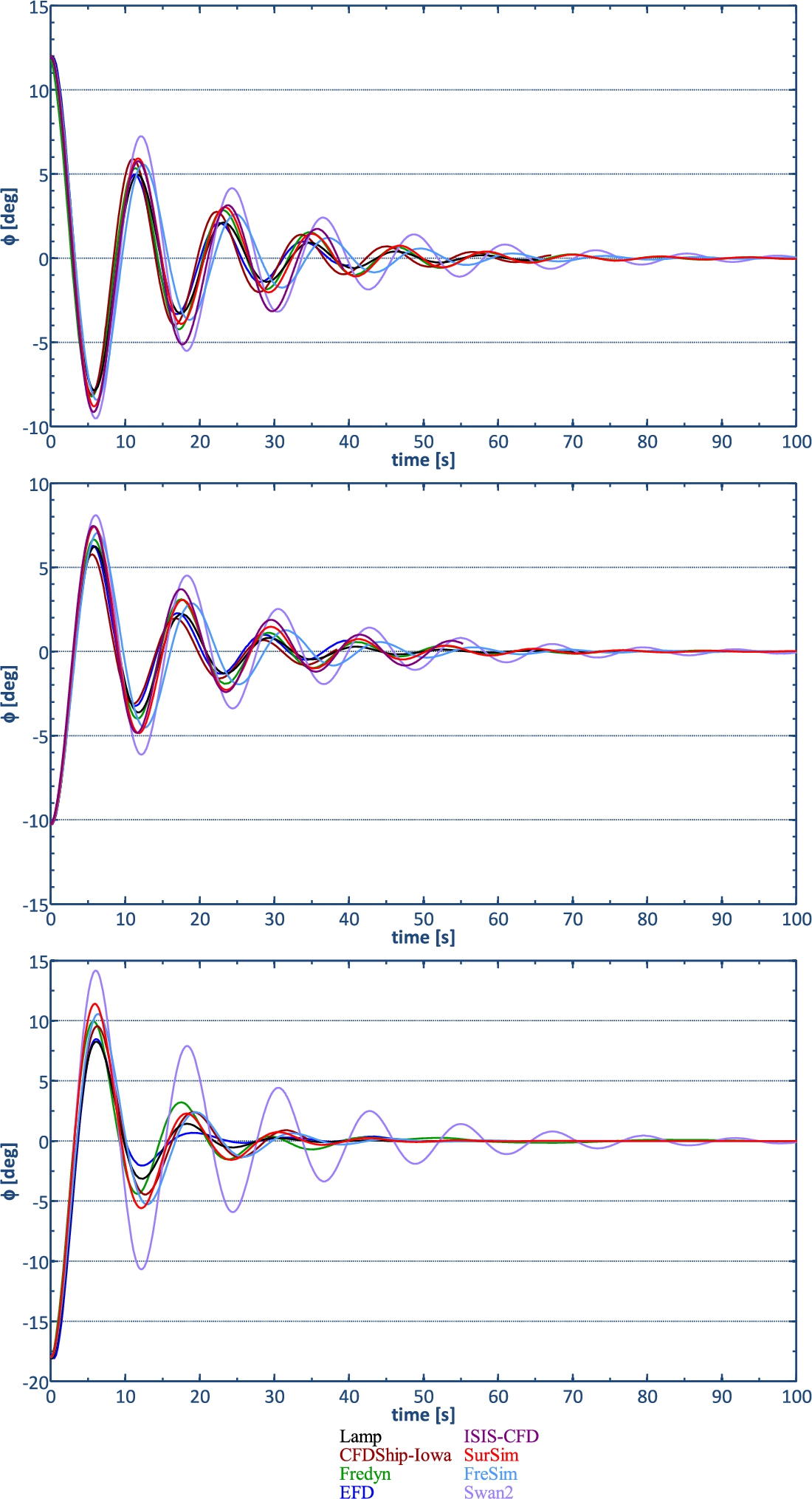
The use of passive fins increases the non-linear damping by 335% compared with the case with no stabilizer fins while the linear damping is similar. Use of active fins results in a three times larger linear damping and a 45% larger non-linear damping compared to the case with passive fins. The non-linear damping with active fins is almost 5 times the non-linear damping of the case without fins.
Comparing all the computed motions with the EFD data shows that most CFD, PF and SB methods predict the roll decay time history fairly well. The effects of passive or active stabilizing fins is reasonably well predicted by all methods.
For the case without fins and the case with passive fins, the roll period is over-predicted by up to 10.8%D. With active fins, the prediction of the period is closer to the experimental one and within 6%D, but this is mainly because there were no predictions made with ISIS-CFD or SWAN2. Generally, the best predictions in terms of damping and period are found for LAMP and CFDShip-Iowa, and the largest for SWAN2. It is difficult to conclude whether the use of CFD, PF or SB is best: CFDShip-Iowa shows good predictions, while ISIS-CFD under predicts the roll damping, probably due to the neglect of the autopilot action. The LAMP or Fredyn results are reasonable, while SWAN2 does not predict roll damping accurately. Generally, Sursim shows reasonable roll decay, while the damping predicted by FreSim is good, but the period is too large.
The prediction errors for the linear and quadratic damping coefficients in many cases show large comparison errors. Often, under predictions in the linear damping coefficients are compensated by an over prediction of the quadratic damping and vice versa. Therefore, it is not possible to judge these coefficients independently. Overall, the results show that with a careful setup of the computations, high-fidelity methods such as CFD appear to better predict the nonlinearities and complex physics associated with roll decay. It should be noted that in PF and SB methods the viscous roll damping, which is caused by hull friction and eddies generated by hull, bilge keels and other appendages, is included using empirical models. The roll damping in LAMP was tuned using the experimental results and obviously the roll decay is predicted well as a result. In the SWAN2 predictions only the wave and lift damping was modeled and the viscous damping was not included. Furthermore, the fins were not set to active mode. Therefore large comparison errors are found.
6.3.Forced roll in calm water
6.3.1.Rudder induced roll with passive fins
The results for rudder-induced roll with passive fins are shown in Table 4 and Fig. 4. The roll response shows only first harmonic oscillations at TR with amplitude of 0.464δ due to the first order rudder/yaw and roll coupling. The yaw motion oscillates mainly at TR with amplitude of 0.018δ and 236 deg phase lag with rudders due to the ship inertia and lethargy. The first order coupling of sway motion with yaw causes harmonic oscillations on side motions with amplitude of 0.24 m at TR.
Table 4
FFT of ship motions and rudder angle for forced roll induced by rudders with passive fins
| Value | EFD | CFDShip-Iowa | Fredyn | LAMP | FreSim | SurSim | ||||||||||||
| a1 | Phase | Phase | Phase | Phase | Phase | Phase | ||||||||||||
| E%D | E%D | E%2π | E%D | E%D | E%2π | E%D | E%D | E%2π | E%D | E%D | E%2π | E%D | E%D | E%2π | ||||
| δ | 13.4 | 0.003 | 0 | −4.5 | 0 | 0 | −11.9 | 0 | 0 | −6.5 | 0 | 0 | −10.2 | 0 | 0 | −10.2 | 0 | 0 |
| ϕ/δ | 0.464 | 0.001 | 137 | −30 | 0 | 5.6 | −58.2 | 0 | 10.8 | −6.3 | 0 | 5.8 | −13.5 | 0 | 11.1 | −41.9 | 0 | 0.8 |
Table 5
FFT of ship motions and rudder angle for forced roll induced by rudders with active fins
| Value | EFD | CFDShip-Iowa | Fredyn | FreSim | SurSim | ||||||||||
| a1 | Phase | Phase | Phase | Phase | Phase | ||||||||||
| E%D | E%D | E%2π | E%D | E%D | E%2π | E%D | E%D | E%2π | E%D | E%D | E%2π | ||||
| δ | 13.43 | 0.002 | 0 | −4.2 | 0 | 0 | −11.6 | 0 | 0 | −10.0 | 0 | 0 | −10.0 | 0 | 0 |
| 0.737 | 0.009 | 27 | −34.3 | 0 | 1.7 | −92.0 | 0 | 6.9 | −34.3 | 0 | 5.3 | −60.5 | 0 | −1.9 | |
| 0.274 | 0.004 | 132 | −34.2 | 0 | 5.3 | −93.4 | 0 | 8.9 | −35.8 | 0 | 7.8 | −62.4 | 0 | 0.6 | |
Table 6
FFT of ship motions and rudder angle for forced roll induced by fins
| Value | EFD | CFDShip-Iowa | Fredyn | LAMP | FreSim | SurSim | ||||||||||||
| a1 | a2/a1 | Phase | Phase | Phase | Phase | Phase | Phase | |||||||||||
| E%D | E%D | E%2π | E%D | E%D | E%2π | E%D | E%D | E%2π | E%D | E%D | E%2π | E%D | E%D | E%2π | ||||
| 25.48 | 0 | 0 | 1.8 | 0 | 0 | 1.8 | 0 | 0 | 1.9 | 0 | 0 | 2.4 | 0 | 0 | 2.4 | 0 | 0 | |
| 0.01 | 0.075 | 18 | 25.2 | 0.1 | −81.7 | NA | NA | NA | −231.6 | 0 | −0.3 | NA | NA | NA | NA | NA | NA | |
| 0.252 | 0.002 | 300 | 13.0 | 0 | 3.6 | 39.6 | 0 | 7.5 | 24.3 | 0 | 4.7 | 41.5 | 0 | 12.2 | 31.6 | 0 | 3.1 | |
Fig. 4.
Forced roll: Rudder, passive fins (top), rudder, active fins (middle), fins (bottom).
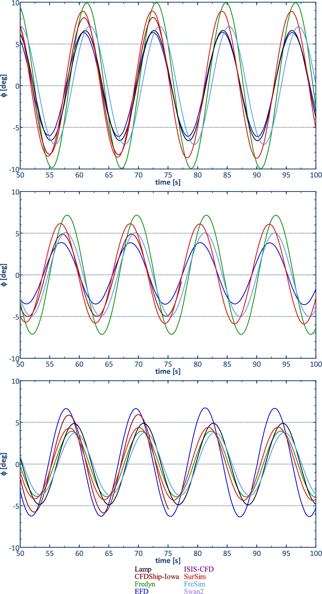
All numerical methods show roll oscillations at TR. However, the roll amplitude is over predicted by all of the methods with E = 6–58%D suggesting under prediction of roll damping and/or over prediction of roll moment due to the rudder action. Fredyn has the maximum over-prediction while the best agreement is for LAMP as the damping could be tuned properly to EFD value. FreSim was not tuned and showed an over prediction of the amplitude of 13.5%D. The roll phase is also predicted within E = 0.8–10.8%2π.
6.3.2.Rudder induced roll with active fins
Table 5 and Fig. 4 show the results for forced roll motion induced by rudders while the fins are active to control the roll motion. The forced rudder motions induce roll oscillations at TR with the amplitude of 3.7 deg, compared to 6.2 deg roll amplitude for previous test with passive fins. The fins are controlled by
The roll motion in the simulations is over predicted for all methods within E = 34–93%D with minimum error for CFDShip-Iowa and maximum error for Fredyn. Fredyn also shows large errors for the roll phase. The fin angles are over predicted as well since the fin angles are correlated with the roll angle.
Compared to the case with passive fins, the FreSim prediction of the roll amplitude deteriorates. The over prediction of the roll amplitude increases to 36%D. This means that the roll moments generated by the fins is under predicted by FreSim.
6.3.3.Fins induced roll
Unlike the two previous cases where the roll was induced by forced rudder motion, the forced roll motion can be provided by harmonically moving the fins. During these tests, the rudders were set to autopilot mode to avoid too large course deviations.
Table 6 and Fig. 4 show the EFD and numerical results for forced roll induced by fins. The oscillatory motion of the fins creates a roll motion with amplitude of 6.43 deg and 60 deg phase lag with the fin motion.
Table 7
FFT of ship motions and rudder and fin angles for regular head waves,
| Value | EFD | CFDShip-Iowa | Fredyn | LAMP | SWAN2 | ||||||||||
| a1 | a2/a1 | Phase | Phase | Phase | Phase | Phase | |||||||||
| E%D | E%D | E%2π | E%D | E%D | E%2π | E%D | E%D | E%2π | E%D | E%D | E%2π | ||||
| 19.34 | 0.498 | 7 | 1.7 | 0.5 | 1.4 | −2.6 | 0.5 | 1.4 | 2.7 | 0.5 | −98.1 | 1.3 | 0.5 | 1.4 | |
| 0.753 | 0.008 | 56 | −1.3 | 0 | −82.5 | 0.8 | 0 | −82.2 | −25.6 | 0 | 15 | 4.9 | 0 | 15.6 | |
| 0.808 | 0.008 | 274 | −7.6 | 0 | 15.3 | 10.5 | 0 | 13.6 | −4.1 | 0 | 15.3 | 3.3 | 0 | 15 | |
The roll angle amplitude as computed by the numerical tools is under predicted by all methods with E = 13–42%D with minimum and maximum error obtained by CFDShip-Iowa and FreSim, respectively. The phase difference between roll and fin motions is under predicted by all methods, with the smallest error of 3.1%D by SurSim and the largest error found for FreSim with E > 12%D. Looking back at the rudder oscillation test with active fins, this confirms that in FreSim the action of the fins is under predicted.
Fig. 5.
Regular head waves,
6.4.Seakeeping in waves
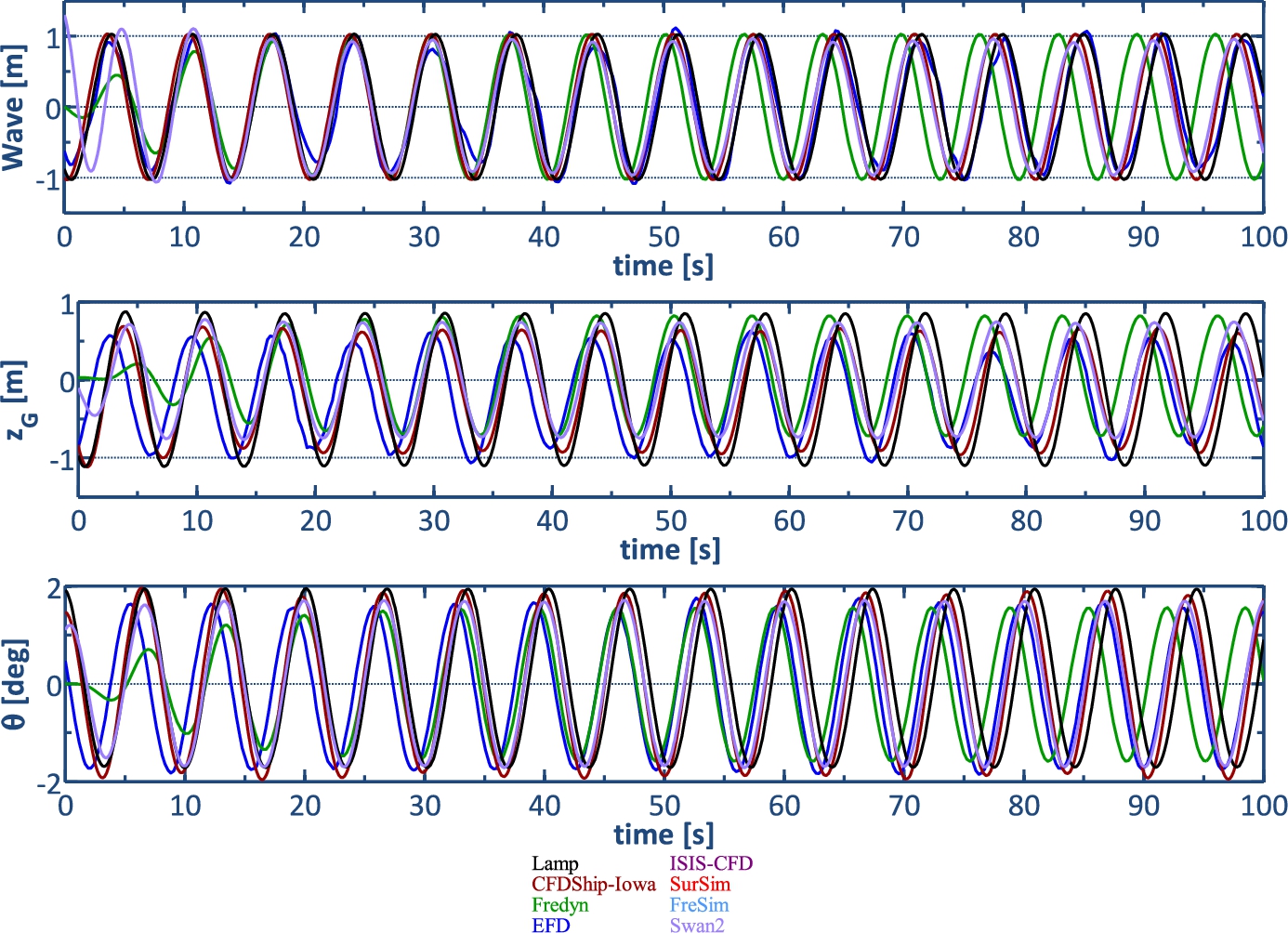
6.4.1.Regular head waves with active fins
The results of the case of seakeeping in regular head waves are shown in Table 7 and Fig. 5. The ship is subjected to a wave with amplitude of 1.03 m and frequency of 0.6 rad/s (
Note that the SB methods could not be used for wave cases, as their mathematical models are only suitable for calm water. Also, ISIS-CFD is not used and the rudders and fins are passive for the SWAN2 simulations. In addition, the roll and yaw motions (as well as dynamic fin and rudder) are not considered in the Fredyn and LAMP computations since the ship is assumed to sail in head waves while the CFDShip-Iowa and SWAN2 computations allow small heading deviations and subsequently predict roll and yaw motions. The time history of the wave shows that all methods follow the EFD in terms of phase and period except Fredyn. In Fredyn, the ship speed is over predicted and encounter period is under predicted. This is caused by an imbalance of the given RPM and the corresponding ship speed. The amplitude of pitch motion is quite well predicted by all methods, with largest error of 11%D by Fredyn. The phase of pitch motion is not predicted well for all methods showing about 50 deg phase lag. For heave motion, the mean value is well predicted for all methods. The comparison error in heave amplitude is within 5%D, except for LAMP, for which an over prediction of 26%D is found. The results show about 60 deg phase lag for all heave predictions compared with EFD data.
6.4.2.Regular beam waves with active fins
The EFD results for seakeeping in regular beam waves are shown in Table 8 and Fig. 6. The wave amplitude is 0.96 m and the wave frequency is 0.8 rad/sec (
Table 8
FFT of ship motions and rudder and fin angles for regular beam waves,
| Value | EFD | CFDShip-Iowa | Fredyn | LAMP | SWAN2 | ||||||||||
| a1 | a2/a1 | Phase | Phase | Phase | Phase | Phase | |||||||||
| E%D | E%D | E%2π | E%D | E%D | E%2π | E%D | E%D | E%2π | E%D | E%D | E%2π | ||||
| 0.325 | 0.047 | 151 | 11.2 | 0.1 | −18.6 | −161.6 | 0 | −12.2 | −331.1 | 0 | −1.7 | NA | NA | NA | |
| 2.833 | 0.001 | 25 | 31.2 | 0 | −1.1 | 44.6 | 0.1 | −7.5 | 21 | 0 | −5.3 | NA | NA | NA | |
| 24.448 | 0.499 | 10 | −0.7 | 0.5 | 1.7 | −4.5 | 0.5 | −96.4 | 2.1 | 0.5 | 2.8 | 1.5 | 0.5 | −96.9 | |
| 0.717 | 0.02 | 266 | −8.6 | 0 | −2.5 | 3.8 | 0 | −3.6 | 5.1 | 0 | −2.2 | 4.2 | 0 | −10.3 | |
| 1.061 | 0.002 | 345 | −1 | 0 | −1.7 | 13.7 | 0 | −3.1 | −2.5 | 0 | −3.9 | 7 | 0 | 95 | |
| 0.71 | 0.002 | 137 | 31.4 | 0 | 4.2 | 44.8 | 0 | −1.4 | 21.2 | 0 | 0.8 | 30.4 | 0 | 17.5 | |
| 0.025 | 0.182 | 121 | 9.1 | 0.1 | −3.3 | −202.3 | 0 | −56.1 | 25 | 0.1 | −3.1 | −38.6 | 0 | −64.4 | |
| 0.025 | 0.052 | 306 | 6.7 | 0.1 | −0.8 | −91 | 0 | 7.5 | −70.8 | 0 | −6.1 | −78.7 | 0 | 6.7 | |
Fig. 6.
Regular beam waves,
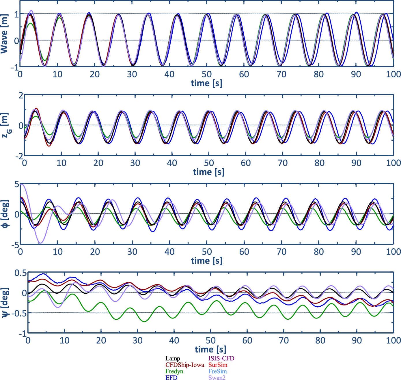
The results for different predictions shown in Fig. 6 indicate that the generated waves follow closely the experimental data in terms of the amplitude and phase. The roll motion shows that all methods under predict the roll amplitude with E = 21–45%D. The best agreement is for LAMP and the largest under prediction is for Fredyn, as shown in Table 8. The roll phase is predicted within E = 0.8–17%D with the largest error for SWAN2. Since the roll is under predicted, the fin angle is also under predicted by all methods. The yaw motion shows oscillations at Te for all prediction methods while the amplitude is over predicted by PF methods with E > 70%D compared to E = 6.7%D for the CFD method, showing that the yaw damping is not properly modeled in PF methods. In addition, the trend of yaw motion (mean value) is not predicted by PF methods. The amplitude of oscillations at Te is predicted for side motion by all methods but the mean value and the trend is only predicted well by CFDShip-Iowa. For pitch response, the amplitude is predicted fairly well by CFDShip-Iowa (E = 9%D) while all PF methods show large errors with E > 25%D. The pitch phase is not predicted well by Fredyn and SWAN2 while CFDShip-Iowa and LAMP show E = 3%D. For heave amplitude, PF methods show E = 2.5–14%D while CFDShip-Iowa prediction has an error with E = 1%D. The ship speed is quite constant and close to EFD value for all methods except Fredyn, which shows an increase of speed during the run, due to the imbalance of propeller thrust and resistance as before. The rudder angle amplitude shows large errors for PF methods particularly for Fredyn as it is correlated with yaw motion.
6.4.3.Stern-quartering bi-chromatic waves with active fins
The EFD results for seakeeping in bi-chromatic waves are shown in Fig. 7. The bi-chromatic wave consists of two regular waves with same amplitude of 1.77 m and periods of 9.4 sec (
Fig. 7.
Stern-quartering bi-chromatic waves.
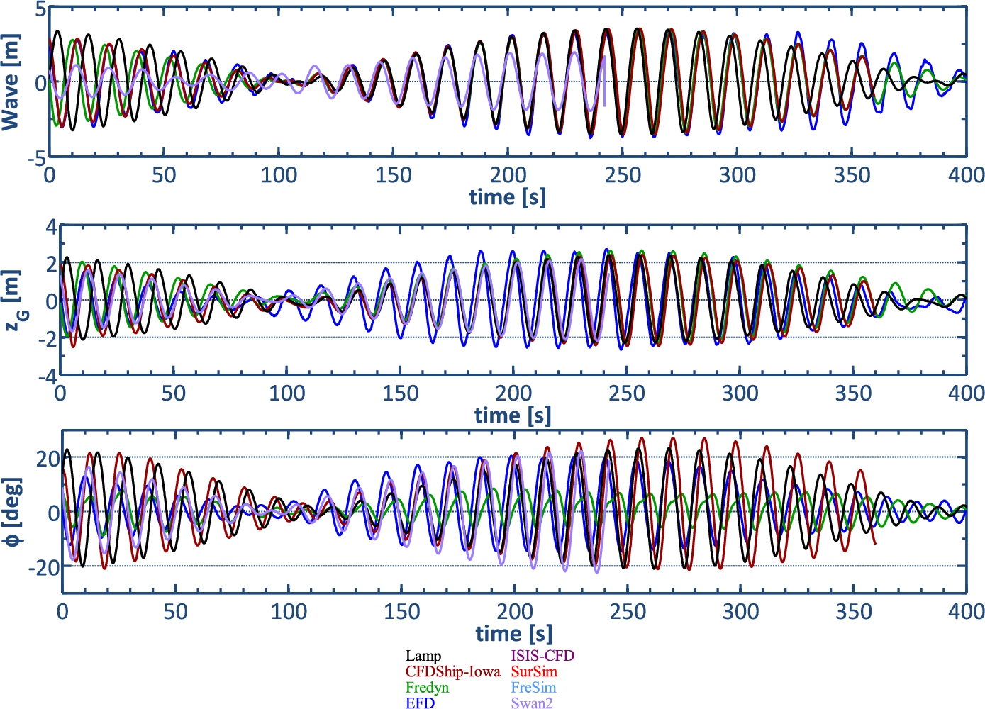
The predictions for different methods are shown in Fig. 7 as well. The wave at the center of gravity shows a phase lag compared to EFD for most predictions due to differences in ship speed. The predictions for roll show that LAMP, SWAN2 and CFDShip-Iowa over predict the roll angle but Fredyn under predicts the roll considerably. Since the fin angle prediction is correlated with roll motion prediction, the fin angles are over predicted by all methods except Fredyn. The amplitude of side motion oscillations is only predicted well by CFDShip-Iowa in terms of the mean value and the trend. The yaw motion shows good agreement for CFDShip-Iowa while Fredyn over predicts the yaw oscillations amplitude. LAMP under predicts the yaw amplitudes. For pitch and heave motions, good agreement is observed for all methods. The rudder angle prediction is dependent on the yaw motion prediction such that the agreement for LAMP and Fredyn predictions are not good. The surge motion and velocity prediction show some differences with EFD. The amplitude of surge velocity oscillations are under predicted by most of methods with the largest errors for the PF methods.
7.Conclusions
SB, PF, and CFD free running simulations were performed for the 5415M in calm water and waves and the results were compared against available experimental data. A detailed validation study was conducted for the motions of the ship and controllers.
The SB methods (FreSim and SurSim) were only applied for roll decay and forced roll in calm water. For roll decay in calm water, the roll motion was predicted reasonably well. The largest errors were found for the case with active fins. For forced roll cases, SB could predict the harmonics induced on ship motions by forced rudder or fins but often showed quite large errors for the amplitudes.
The PF methods (Fredyn, LAMP and SWAN2) are able to accurately predict the roll period during the roll decay cases. The linear roll damping coefficients showed reasonable agreement with the EFD, but large errors were obtained for the non-linear terms suggesting compensation of errors or that nonlinearities are not fully considered in PF methods. For forced roll cases, roll showed similar motions to EFD for all codes but with different amplitudes. The PF methods in waves predicted quite well the amplitude of oscillations on most of motions. Overall, LAMP showed the best results of all PF codes, indicating that a-priori tuning of PF codes using PMM results or experiments improves the predictive capability of the tool considerably. Generally, the amplitudes of coupled motions (roll-yaw, roll-heave or roll-pitch) were poorly predicted by the PF codes.
For the roll decay cases predicted with CFD, the roll period was generally predicted better than with SB and PF codes. The linear roll damping was predicted with the same order of error as PF codes with tuned damping terms but the nonlinear damping showed much better agreement with EFD data. The good prediction of roll and nonlinearities also resulted in good predictions for other motions including heave and pitch. For forced roll cases, CFD could predict the same harmonics as EFD for all motions. The roll amplitude was better predicted compared with SB and PF methods and also other motions are often predicted with less error, in particular for the second harmonics on heave and pitch. For wave cases, the amplitude and phase of the oscillations on most motions were again predicted better than PF methods. Overall, it is concluded that only high fidelity CFD is capable of accurately simulating the physics associated with roll decay, forced roll and sailing in regular or bi-chromatic waves. Despite the additional preparation and computing times involved with CFD compared to SB or PF computations, it is worthwhile to study individual cases of a ship in waves with CFD to obtain better understanding of the physics involved, or to improve the tuning of PF methods before applying them to a wide range of sea states and wave directions.
Acknowledgements
The authors gratefully acknowledge the permission given by the Danish, Italian and Netherlands Navies to use the test results obtained within Supplement Joint Program 10.111 to the Western European Armaments Group Memorandum of Understanding for THALES.
The research by MARIN was partly funded by the Dutch Ministry of Economic Affairs. Computations with ISIS-CFD were performed using HPC resources from GENCI-IDRIS (Grant2009-x2009021308), which is gratefully acknowledged. The research performed at IIHR was sponsored by the US Office of Naval Research grant N000141010017 under administration of Dr. Thomas Fu. The CFD simulations were conducted utilizing DoD HPC.
References
[1] | M. Araki, H. Sadat-Hosseini, Y. Sanada, K. Tanimoto, N. Umeda and F. Stern, Estimating maneuvering coefficients using system identification methods with experimental, system-based, and CFD free-running trial data, Ocean Engineering 51: ((2012) ), 63–84. doi:10.1016/j.oceaneng.2012.05.001. |
[2] | M. Araki, H. Sadat-Hosseini, Y. Sanada, N. Umeda and F. Stern, Study of system-based mathematical model using system identification method with experimental, CFD, and system-based free-running trials in wave, in: 11th International Conference on the Stability of Ships and Ocean Vehicles, Athens, Greece, (2012) , pp. 23–28. |
[3] | H. Boonstra, M.P. de Jongh and L. Pallazi, Safety assessment of small container feeders, in: 9th Symposium on Practical Design of Ships and Other Floating Structures (PRADS), Lübeck-Travemünde, Germany, (2004) . |
[4] | T.H.J. Bunnik, E.F.G. van Daalen, G.K. Kapsenberg, Y. Shin, R.H.M. Huijsmans, G. Deng, G. Delhommeau, M. Kashiwagi and B. Beck, A comparative study on state-of-the-art prediction tools for seakeeping, in: 28th Symposium on Naval Hydrodynamics, Pasadena, California, (2010) , pp. 12–17. |
[5] | N.F. Carette and F. van Walree, Calculation method to include water on deck effects, in: 11th International Ship Stability Workshop (ISSW), Wageningen, The Netherlands, (2010) , pp. 166–172. |
[6] | P.M. Carrica, F. Ismail, M. Hyman, S. Bhushan and F. Stern, Turn and zigzag maneuvers of a surface combatant using a URANS approach with dynamic overset grids, Journal of Marine Science and Technology 18: ((2013) ), 166–181. doi:10.1007/s00773-012-0196-8. |
[7] | J.O. de Kat and J.R. Paulling, Prediction of extreme motions and capsizing of ships and offshore marine vehicles, in: 20th International Conference on Offshore Mechanics and Arctic Engineering (OMAE), Rio de Janeiro, Brazil, (2001) , paper number OMAE2001/OFT-1280. |
[8] | R. Duvigneau, M. Visonneau and G.B. Deng, On the role played by turbulence closures in hull shape optimization at model and full scale, Journal of Marine Science and Technology 8: ((2003) ), 11–25. doi:10.1007/s10773-003-0153-8. |
[9] | Y. Himeno, Prediction of Ship Roll Damping, State of the Art, University of Michigan, Report No. 239, 1981. |
[10] | J. Holtrop and G.G.J. Mennen, An approximate power prediction method, International Shipbuilding Progress 29: (335) ((1982) ), 166–170. doi:10.3233/ISP-1982-2933501. |
[11] | J.P. Hooft, The cross flow drag on a maneuvering ship, Ocean Engineering 21: (3) ((1994) ), 329–342. doi:10.1016/0029-8018(94)90004-3. |
[12] | J. Huang, P. Carrica and F. Stern, Semi-coupled air/water immersed boundary approach for curvilinear dynamic overset grids with application to ship hydrodynamics, International Journal for Numerical Methods in Fluids 58: ((2008) ), 591–624. doi:10.1002/fld.1758. |
[13] | D.C. Kring, Y.F. Huang, P.D. Sclavounos, T. Vada and A. Braathen, Nonlinear ship motions and wave induced loads by a Rankine panel method, in: 21st Symposium of Naval Hydrodynamics, Trondheim, (1996) , pp. 45–63. |
[14] | A. Leroyer and M. Visonneau, Numerical methods for RANSE simulations of a self-propelled fish-like body, Journal of Fluids & Structures 20: (7) ((2005) ), 975–991. doi:10.1016/j.jfluidstructs.2005.05.007. |
[15] | M. Levadou and G. Gaillarde, Operational guidance to avoid parametric roll, in: RINA – Container Vessels Conference, (2003) . |
[16] | W.M. Lin, S. Zhang, K. Weems and D. Liut, Numerical Simulations of Ship Maneuvering in Waves, in: 26th Symposium on Naval Hydrodynamics, Rome, Italy, (2006) . |
[17] | W.M. Lin, S. Zhang, K. Weems and D.K.P. Yue, A mixed source formulation for nonlinear ship-motion and wave-load simulations, in: 7th International Conference on Numerical Ship Hydrodynamics, Nantes, France, (1999) , pp. 1.3-1–1.3-12. |
[18] | S.M. Mousaviraad, S. Bhushan and F. Stern, CFD prediction of free-running SES/ACV deep and shallow water maneuvering in calm water and waves, in: MARSIM, Singapore, (2012) . |
[19] | F.H.H.A. Quadvlieg, E. Armaoğlu, R. Eggers and P. van Coevorden, Prediction and verification of the maneuverability of naval surface ships, in: SNAME Annual Meeting and Expo, Seattle/Bellevue, WA, (2010) . |
[20] | P. Queutey and M. Visonneau, An interface capturing method for free-surface hydrodynamic flows, Computers & Fluids 36: (9) ((2007) ), 1481–1510. doi:10.1016/j.compfluid.2006.11.007. |
[21] | H. Sadat-Hosseini, M. Araki, N. Umeda, M. Sano, D.J. Yeo, Y. Toda and F. Stern, CFD, system-based method, and EFD investigation of ONR tumblehome instability and capsize with evaluation of the mathematical model, in: 12th International Ship Stability Workshop (ISSW), (2011) , pp. 135–145. |
[22] | H. Sadat-Hosseini, P.M. Carrica, F. Stern, N. Umeda, H. Hashimoto, S. Yamamura and A. Mastuda, CFD, system-based and EFD study of ship dynamic instability events: Surf-riding, periodic motion, and broaching, Journal of Ocean Engineering 38: (1) ((2011) ), 88–110. doi:10.1016/j.oceaneng.2010.09.016. |
[23] | H. Sadat-Hosseini, D.H. Kim, S.L. Toxopeus, M. Diez and F. Stern, CFD and Potential Flow Simulations of Fully Appended Free Running 5415M in Irregular Waves, in: World Maritime Technology Conference (WMTC), Providence, RI, (2015) . |
[24] | H. Sadat-Hosseini, Y. Sanada and F. Stern, Experiments and CFD for ONRT Course Keeping in Regular Waves, SNAME Transactions (2016). |
[25] | H. Sadat-Hosseini and F. Stern, System based and CFD simulations of 5415M maneuvering, in: Verification and Validation of Ship Maneuvering Simulation Method Workshop (SIMMAN), Lyngby, Denmark, (2014) . |
[26] | H. Sadat-Hosseini, F. Stern, A. Olivieri, E.F. Campana, H. Hashimoto, N. Umeda, G. Bulian and A. Francescutto, Head-wave parametric rolling of a surface combatant, Ocean Engineering 37: ((2010) ), 859–878. doi:10.1016/j.oceaneng.2010.02.010. |
[27] | H. Sadat-Hosseini, P.C. Wu and P.M. Carrica Stern F, CFD simulations of KVLCC2 maneuvering with different propeller modeling, in: Verification and Validation of Ship Maneuvering Simulation Method Workshop (SIMMAN), Lyngby, Denmark, (2014) . |
[28] | T. Sato, K. Izumi and H. Miyata, Numerical Simulation of Maneuvering motion, in: 22nd Symposium on Naval Hydrodynamics, Fukuoka, Japan, (1998) , pp. 724–737. |
[29] | P.D. Sclavounos, Computation of Wave Ship Interactions, M. Qhkusu, ed., Advances in Marine Hydrodynamics, Computational Mechanics Publication, (1996) . |
[30] | F. Stern, K. Agdrup, S.Y. Kim A. Cura Hochbaum, K.P. Rhee, F.H.H.A. Quadvlieg, P. Perdon, T. Hino, R. Broglia and J. Gorski, Experience from SIMMAN 2008-the first workshop on verification and validation of ship maneuvering simulation methods, Journal of Ship Research 55: ((2011) ), 135–147. |
[31] | SWAN2 User Manual, Ship Flow Simulation in Calm Water and in Waves, Boston Marine Consulting Inc., Boston, MA 02116, USA, (2002) . |
[32] | S.L. Toxopeus, Validation of slender-body method for prediction of linear maneuvering coefficients using experiments and viscous-flow calculations, in: 7th ICHD International Conference on Hydrodynamics, Ischia, Italy, (2006) , pp. 589–598. |
[33] | S.L. Toxopeus, Practical application of viscous-flow calculations for the simulation of manoeuvring ships, PhD thesis, Delft University of Technology, 2011. ISBN 978-90-75757-05-7. |
[34] | S.L. Toxopeus and S.W. Lee, Comparison of maneuvering simulation programs for SIMMAN test cases, in: SIMMAN 2008 Workshop on Verification and Validation of Ship Maneuvering Simulation Methods, Copenhagen, Denmark, (2008) , pp. E56–61. |
[35] | S.L. Toxopeus, F. van Walree and R. Hallmann, Maneuvering and Seakeeping Tests for 5415M, in: AVT-189 Specialists’ Meeting, Portsdown West, UK, (2011) . |
[36] | T. Yen, S. Zhang, K. Weems and W.M. Lin, Development and validation of numerical simulations for ship maneuvering in calm water and in waves, in: 28th Symposium of Naval Hydrodynamics, Pasadena, California, USA, (2010) . |
[37] | T.G. Yen, D.A. Liut, S. Zhang, W.M. Lin and K.M. Weems, LAMP simulation of calm water maneuvers for a US navy surface combatant, in: SIMMAN 2008 Workshop on Verification and Validation of Ship Maneuvering Simulation Methods, Copenhagen, Denmark, (2008) . |


