A comparison study of chi-square and uniform distributions of mesh clients for different router replacement methods using WMN-PSODGA hybrid intelligent simulation system

1.Introduction

The wireless networks and devices are becoming increasingly popular and they provide users access to information and communication anytime and anywhere [2, 10, 13, 16, 20, 23]. Wireless Mesh Networks (WMNs) are gaining a lot of attention because of their low-cost nature that makes them attractive for providing wireless Internet connectivity. A WMN is dynamically self-organized and self-configured, with the nodes in the network automatically establishing and maintaining mesh connectivity among itself (creating, in effect, an ad hoc network). This feature brings many advantages to WMN such as low up-front cost, easy network maintenance, robustness and reliable service coverage [1]. Moreover, such infrastructure can be used to deploy community networks, metropolitan area networks, municipal and corporative networks, and to support applications for urban areas, medical, transport and surveillance systems.

Mesh node placement in WMNs can be seen as a family of problems, which is shown (through graph theoretic approaches or placement problems, e.g. [8, 14]) to be computationally hard to solve for most of the formulations [27].

We consider the version of the mesh router nodes placement problem in which we are given a grid area where to deploy a number of mesh router nodes and a number of mesh client nodes of fixed positions (of an arbitrary distribution) in the grid area. The objective is to find a location assignment for the mesh routers to the cells of the grid area that maximizes the network connectivity, client coverage and consider load balancing for each router. Network connectivity is measured by Size of Giant Component (SGC) of the resulting WMN graph, while the user coverage is simply the number of mesh client nodes that fall within the radio coverage of at least one mesh router node and is measured by Number of Covered Mesh Clients (NCMC). For load balancing, we added in the fitness function a new parameter called NCMCpR (Number of Covered Mesh Clients per Router).

Node placement problems are known to be computationally hard to solve [11, 12, 28]. Machine learning and evolutionary-based algorithms are some practical approaches capable of solving computationally hard problems. These approaches, which have been applied to fields ranging from networking and telecommunications to automation and power control systems [5, 7], are investigated for node placement problems in several previous works [3, 9, 15, 18].

In [21], we implemented a Particle Swarm Optimization (PSO) based simulation system, called WMN-PSO. Also, we implemented another simulation system based on Genetic Algorithm (GA), called WMN-GA [19], for solving node placement problem in WMNs. Then, we designed and implemented a hybrid simulation system based on PSO and Distributed GA (DGA). We call this system WMN-PSODGA.

Using the WMN-PSODGA, we can explore different router replacement methods and various distributions of mesh clients. This is important because each router replacement method does not achieve the same performance on every distribution of mesh clients. Moreover, every distribution of mesh clients yields different results for different WMN applications since the topology of a WMN can vary widely. In this paper, we compare the simulation results of chi-square and uniform distributions of mesh clients for different router replacement methods.

The rest of the paper is organized as follows. In Section 2, we introduce intelligent algorithms. In Section 3 is presented the implemented hybrid simulation system. The simulation results are given in Section 4. Finally, we give conclusions and future work in Section 5.

2.Intelligent algorithms

2.1.Particle swarm optimization

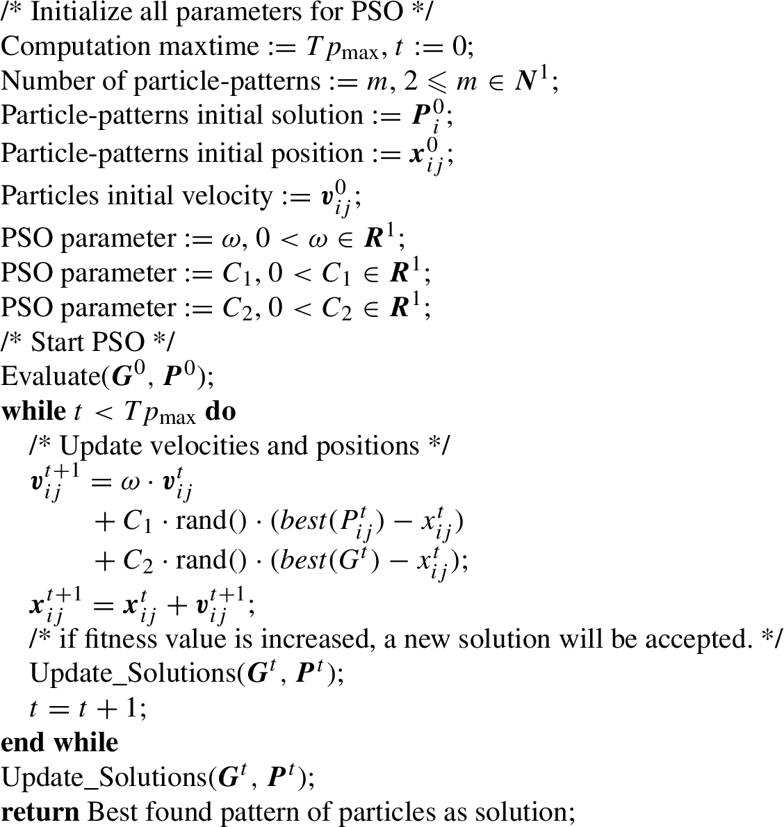
In PSO a number of simple entities (the particles) are placed in the search space of some problem or function and each evaluates the objective function at its current location. The objective function is often minimized and the exploration of the search space is not through evolution [17].

Each particle then determines its movement through the search space by combining some aspect of the history of its own current and best (best-fitness) locations with those of one or more members of the swarm, with some random perturbations. The next iteration takes place after all particles have been moved. Eventually the swarm as a whole, like a flock of birds collectively foraging for food, is likely to move close to an optimum of the fitness function.

Each individual in the particle swarm is composed of three D-dimensional vectors, where D is the dimensionality of the search space. These are the current position x→i, the previous best position p→i and the velocity v→i.

The particle swarm is more than just a collection of particles. A particle by itself has almost no power to solve any problem; progress occurs only when the particles interact. Problem solving is a population-wide phenomenon, emerging from the individual behaviors of the particles through their interactions. In any case, populations are organized according to some sort of communication structure or topology, often thought of as a social network. The topology typically consists of bidirectional edges connecting pairs of particles, so that if j is in i’s neighborhood, i is also in j’s. Each particle communicates with some other particles and is affected by the best point found by any member of its topological neighborhood. This is just the vector p→i for that best neighbor, which we will denote with p→g. The potential kinds of population “social networks” are hugely varied, but in practice certain types have been used more frequently. We show the pseudo code of PSO in Algorithm 1.

In the PSO process, the velocity of each particle is iteratively adjusted so that the particle stochastically oscillates around p→i and p→g locations.

Algorithm 1

Pseudo code of PSO

2.2.Distributed genetic algorithm

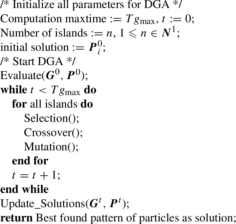
Classic GAs have proved their effectiveness in solving real-world optimization problems. However, in problems with a huge search space and with many local optima, they cannot guarantee success in finding the global optima. To successfully find the global optima, many different approaches can be used in combination with the classic GA. For example, the gradient-descent (GD) technique for local searching and constraints management has demonstrated great feasibility to provide high precision with reduced number of individuals and generations [6]. Distributed Genetic Algorithm (DGA), on the other hand, has shown their usefulness for the resolution of many computationally hard combinatorial optimization problems. We show the pseudo code of DGA in Algorithm 2.

Algorithm 2

Pseudo code of DGA

Population of individuals: Unlike local search techniques that construct a path in the solution space jumping from one solution to another one through local perturbations, DGA use a population of individuals giving thus the search a larger scope and chances to find better solutions. This feature is also known as “exploration” process in difference to “exploitation” process of local search methods.

Fitness: The determination of an appropriate fitness function, together with the chromosome encoding are crucial to the performance of DGA. Ideally we would construct objective functions with “certain regularities”, i.e. objective functions that verify that for any two individuals which are close in the search space, their respective values in the objective functions are similar.

Selection: The selection of individuals to be crossed is another important aspect in DGA as it impacts on the convergence of the algorithm. Several selection schemes have been proposed in the literature for selection operators trying to cope with premature convergence of DGA. There are many selection methods in GA. In our system, we implement 2 selection methods: Random method and Roulette wheel method.

Crossover operators: Use of crossover operators is one of the most important characteristics. Crossover operator is the means of DGA to transmit best genetic features of parents to offsprings during generations of the evolution process. Many methods for crossover operators have been proposed such as Blend Crossover (BLX-α), Unimodal Normal Distribution Crossover (UNDX), Simplex Crossover (SPX).

Mutation operators: These operators intend to improve the individuals of a population by small local perturbations. They aim to provide a component of randomness in the neighborhood of the individuals of the population. In our system, we implemented two mutation methods: uniformly random mutation and boundary mutation.

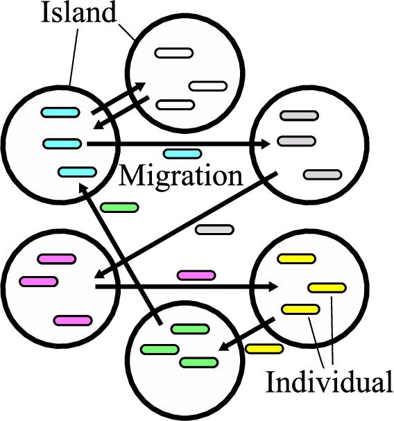
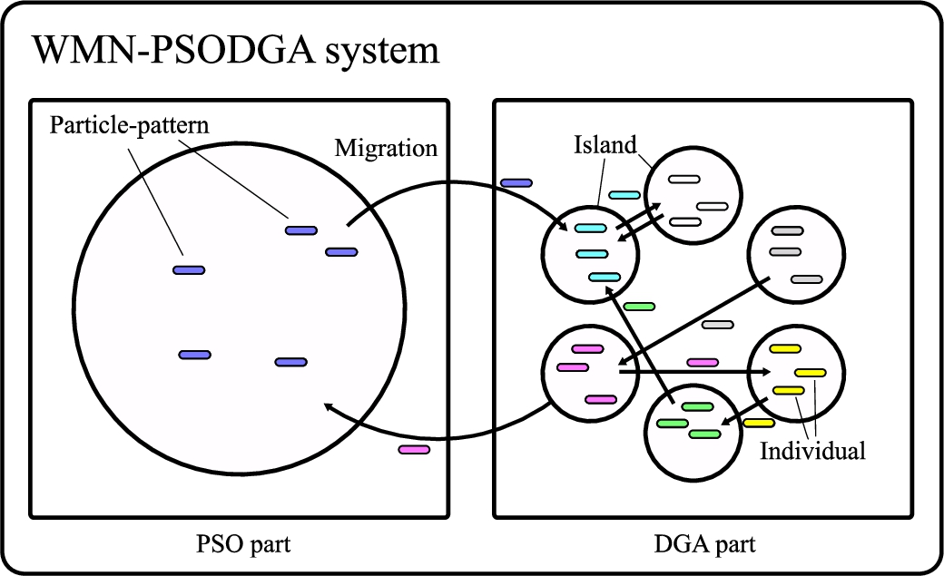
Escaping from local optima: GA itself has the ability to avoid falling prematurely into local optima and can eventually escape from them during the search process. DGA has one more mechanism to escape from local optima by considering some islands. Each island computes GA for optimizing and they migrate its gene to provide the ability to avoid from local optima (see Fig. 1).

Convergence: The convergence of the algorithm is the mechanism of DGA to reach to good solutions. A premature convergence of the algorithm would cause that all individuals of the population be similar in their genetic features and thus the search would result ineffective and the algorithm getting stuck into local optima. Maintaining the diversity of the population is therefore very important to this family of evolutionary algorithms.

Fig. 1.

Model of migration in DGA.

3.Proposed and implemented WMN-PSODGA hybrid intelligent simulation system

In this section, we present the proposed WMN-PSODGA hybrid intelligent simulation system. In the following, we describe the initialization, particle-pattern, gene coding, fitness function, and replacement methods. The pseudo code of our implemented system is shown in Algorithm 3. Also, our implemented simulation system uses Migration function as shown in Fig. 2. The Migration function swaps solutions among lands included in PSO part.

Algorithm 3

Pseudo code of WMN-PSODGA system

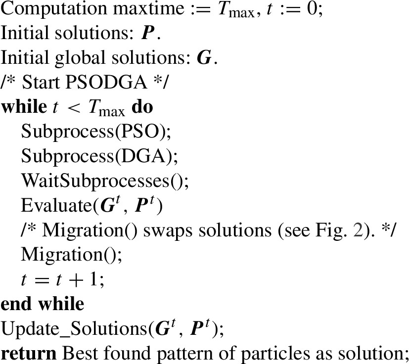
Fig. 2.

Model of WMN-PSODGA migration.

Initialization. We decide the velocity of particles by a random process considering the uniform sampling of the area size. For instance, when the area size is W×H, the velocity is decided randomly from −W2+H2 to W2+H2.

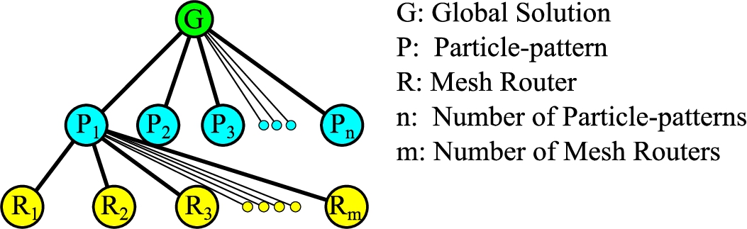
Particle-pattern. A particle is a mesh router. A fitness value of a particle-pattern is computed by combination of mesh routers and mesh clients positions. In other words, each particle-pattern is a solution as shown is Fig. 3.

Fig. 3.

Relationship among global solution, particle-patterns, and mesh routers in PSO part.

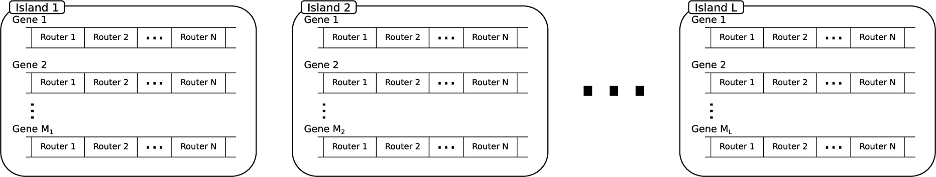
Gene coding. A gene (individual) describes a WMN. As shown in Fig. 4, each individual has its own combination of mesh routers, which includes information about their position and communication distance. In other words, each individual has information over the WMN that can calculate the value of its fitness function. Therefore, each combination of these mesh routers is a solution.

Fig. 4.

Graphical representation of gene coding for a problem with N mesh routers using L islands and M individuals (DGA part).

Fitness function. WMN-PSODGA has the fitness function to evaluate the temporary solution of the router’s placements. The fitness function is defined as:

This function uses the following indicators.

WMN-PSODGA aims to maximize the value of the fitness function in order to optimize the placements of the routers using the above three indicators. Weight-coefficients of the fitness function are α, β, and γ for NCMC, SGC, and NCMCpR, respectively. Moreover, the weight-coefficients are implemented as α+β+γ=1.

Router replacement methods. A mesh router has x, y positions, and velocity. Mesh routers are moved based on velocities. There are many router replacement methods as showing in the following.

4.Simulation results

In this section, we compare the simulation results of chi-square and uniform distributions of mesh clients for different router replacement methods. The weight-coefficients of fitness function were adjusted for optimization. In this paper, the weight-coefficients are α=0.6, β=0.3, γ=0.1. The number of mesh routers is considered 16 and the number of mesh clients 48. Table 1 summarizes the common parameters used for simulation. Figure 5 and Fig. 6 show the visualization results after the optimization for chi-square distribution and uniform distribution, respectively. Figure 7 and Fig. 8 show the number of covered mesh clients by each router. Figure 9 and Fig. 10 show the standard deviation where r is the correlation coefficient.

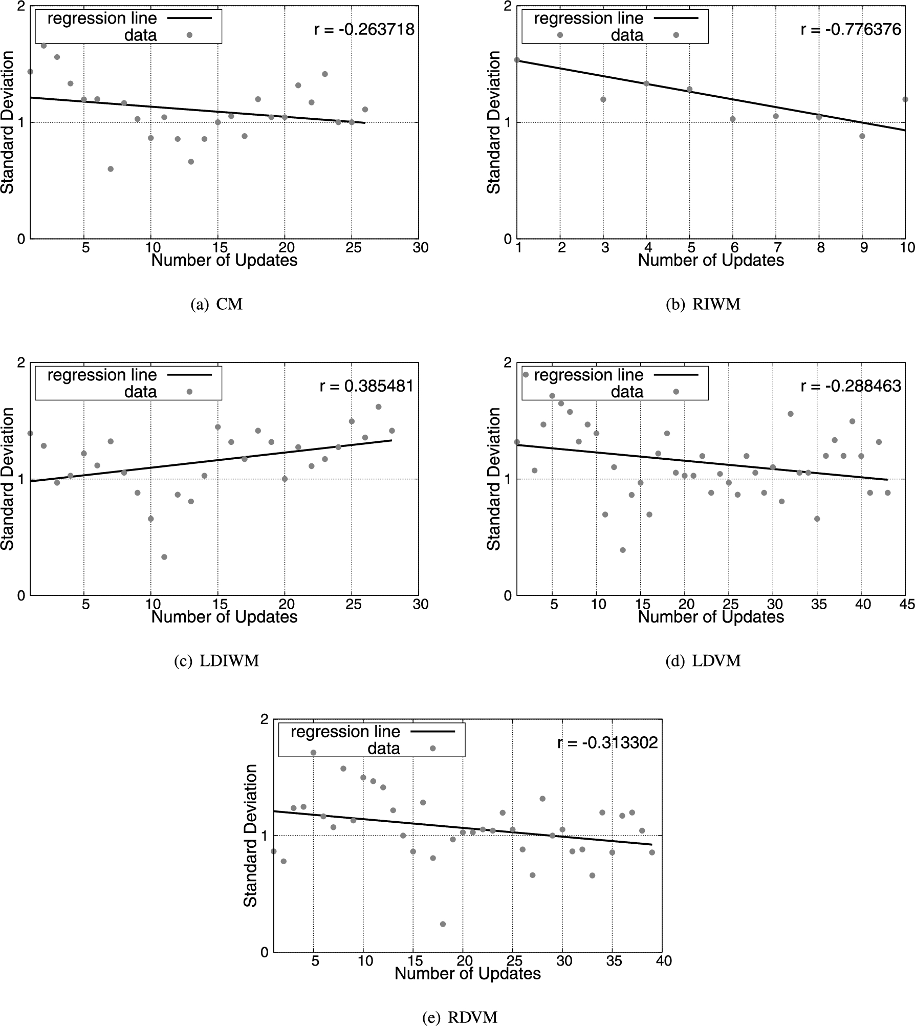
As shown in Fig. 5, when using chi-square distribution, 16 mesh routers can cover all mesh clients for all router replacement methods. On the other hand, in Fig. 6, the simulation results show that for the uniform distribution, 16 mesh routers are not enough to cover all mesh clients regardless of router replacement method used. This can be seen also from Fig. 7 and Fig. 8. In Fig. 9 and Fig. 10, we can see which router replacement methods show better results for load balancing by comparing their standard deviations and their correlation coefficients. When the standard deviation is an increasing line (r>0), the number of mesh clients for each router tends to be different. On the other hand, when the standard deviation is a decreasing line (r<0), the number of mesh clients for each router tends to go close to each other. For chi-square distribution (see Fig. 9), CM, RIWM, LDIWM and LDVM have a positive correlation coefficient r, indicating that each of these router replacement methods does not show good load balancing. For this distribution, the best performance is achieved for RDVM. Figure 10 shows that when using uniform distribution, there are four router replacement methods (CM, RIWM, LDVM and RDVM) that show good load balancing, and only one (LDIWM) has a positive correlation coefficient. Among the four methods that give better results, RIWM is the one outperforming the other methods.

Fig. 5.

Visualization results after the optimization (chi-square distribution).

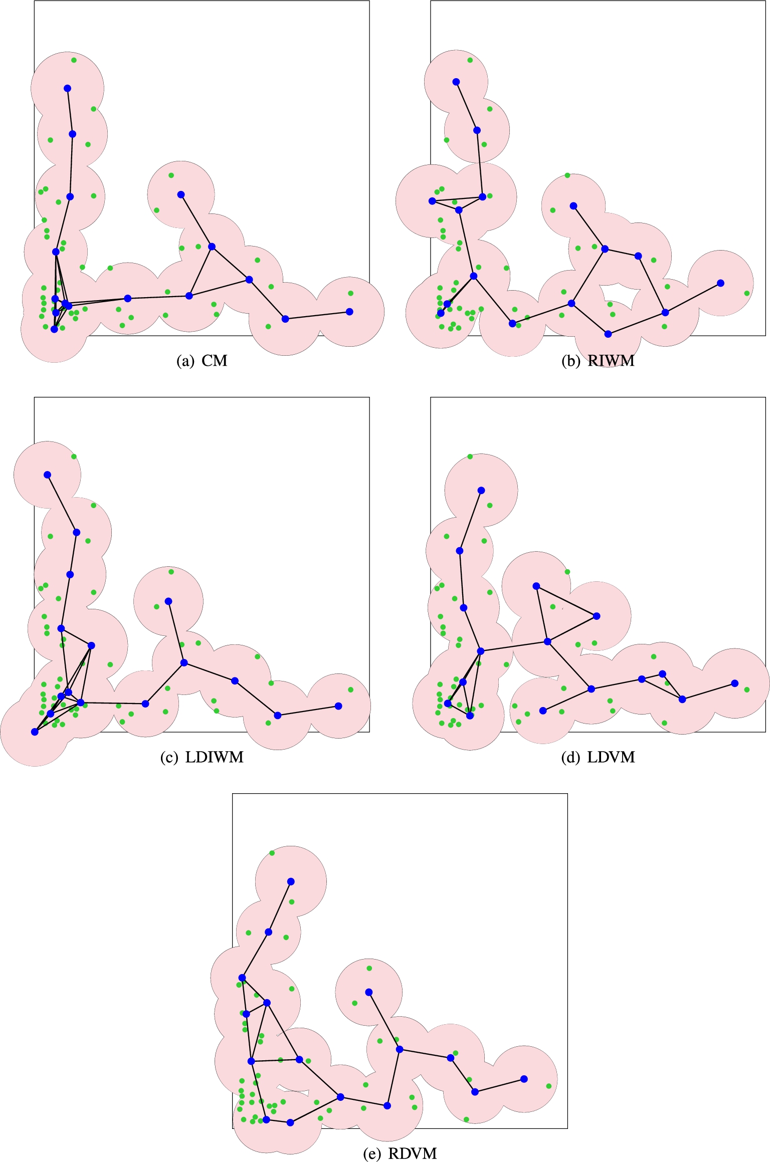
Fig. 6.

Visualization results after the optimization (uniform distribution).

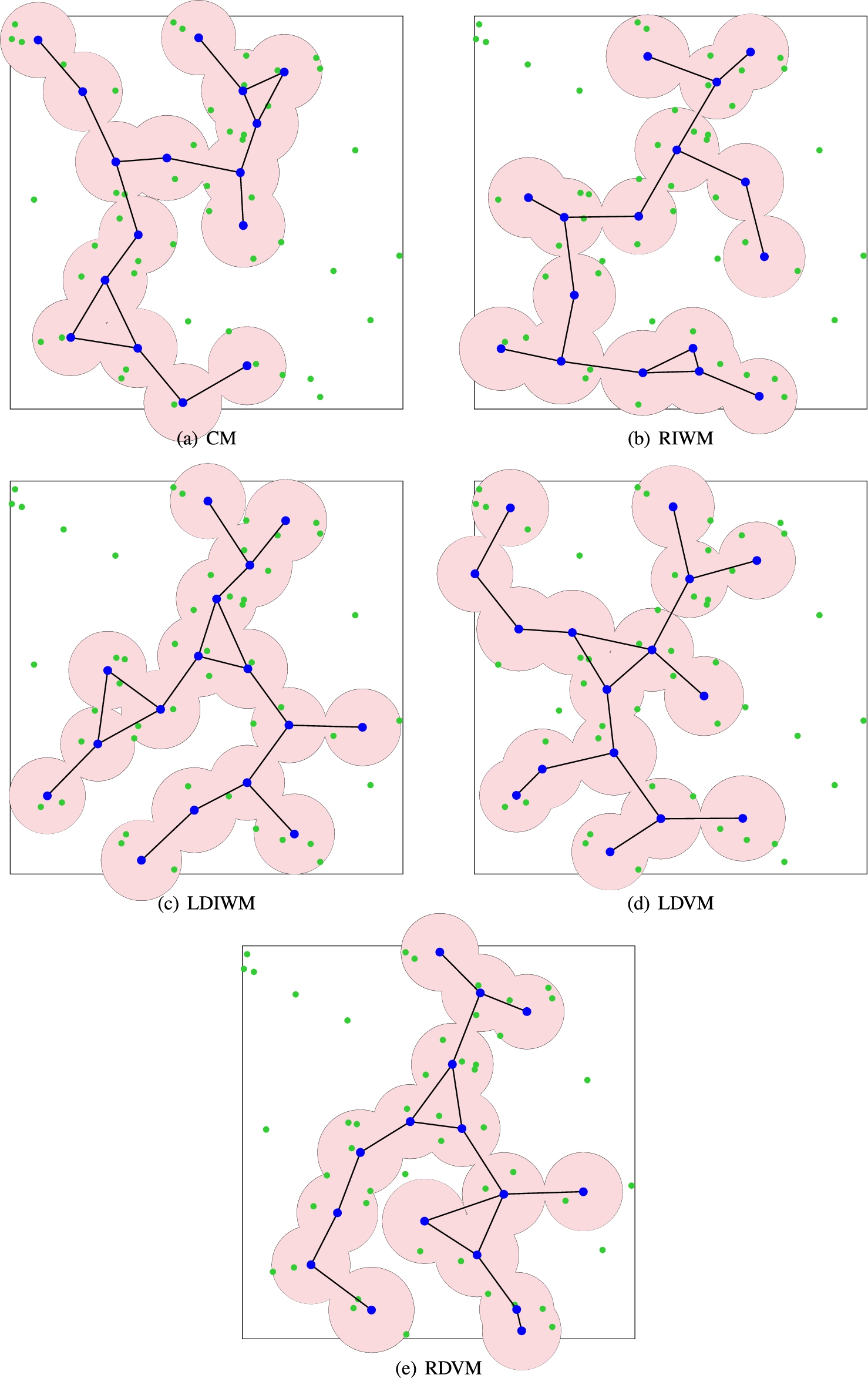
Fig. 7.

Number of covered clients by each router after the optimization (chi-square distribution).

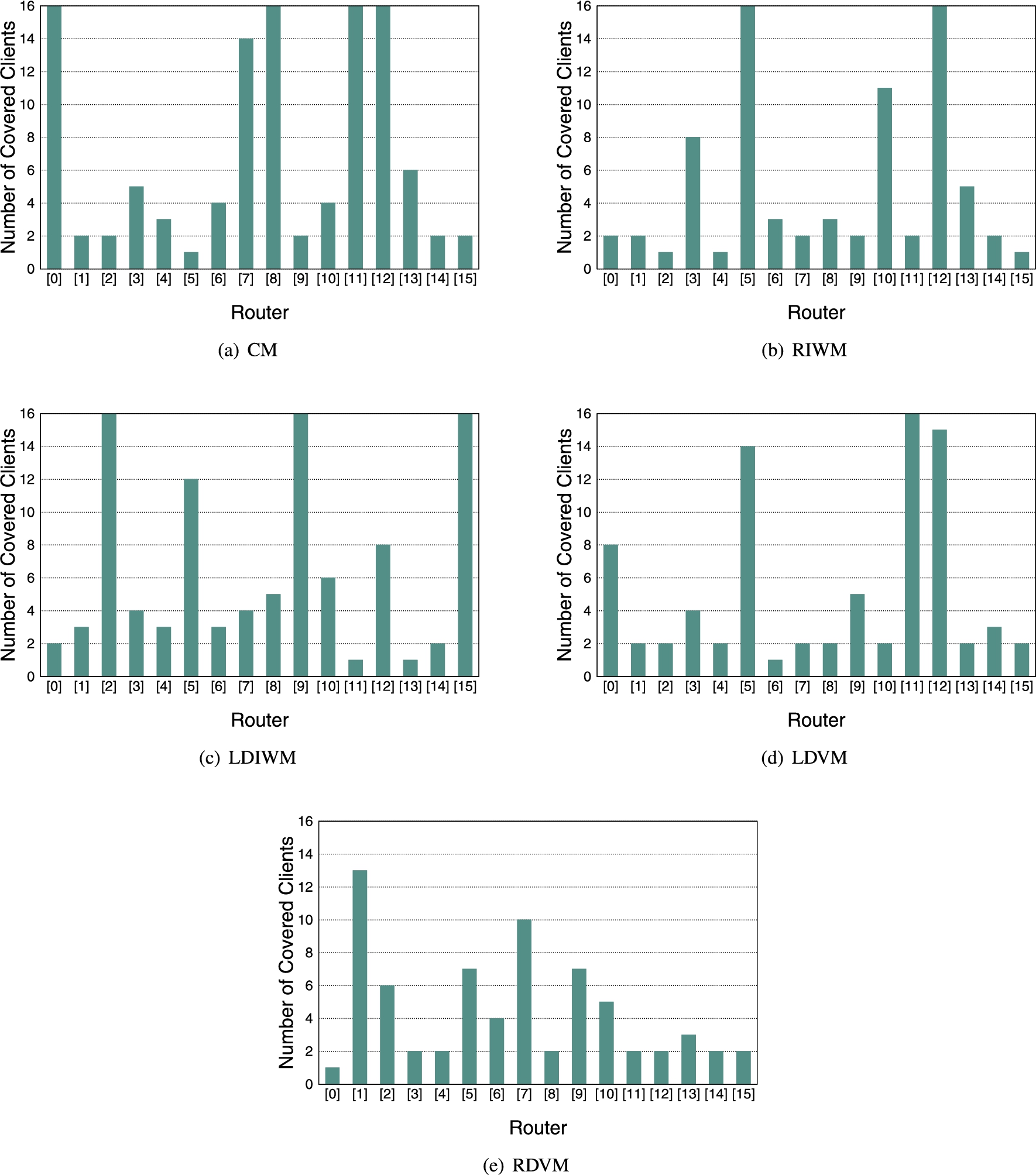
Fig. 8.

Number of covered clients by each router after the optimization (uniform distribution).

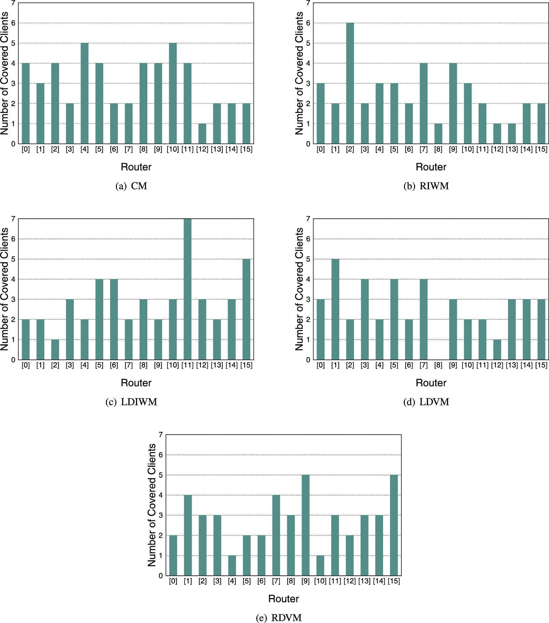
Fig. 9.

Transition of the standard deviations (chi-square distribution).

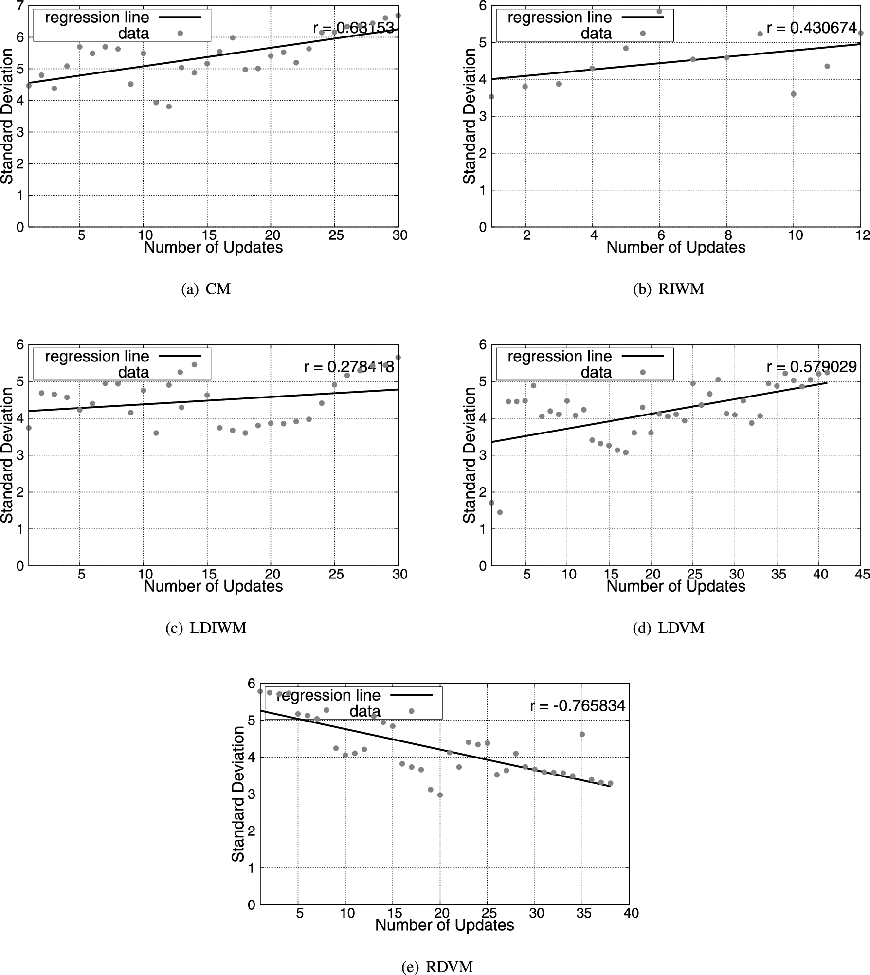
Fig. 10.

Transition of the standard deviations (uniform distribution).

5.Conclusions

In this work, we evaluated the performance of WMNs using a hybrid intelligent simulation system based on PSO and DGA (called WMN-PSODGA). We compared the simulation results of chi-square and uniform distributions of mesh clients for different router replacement methods: CM, RIWM, LDIWM, LDVM and RDVM.

The simulation results show that the uniform distribution makes a good load balancing for four router replacement methods, but the mesh routers do not cover all mesh clients. On the other hand, in terms of load balancing, the only method that shows poor results for this distribution is LDIWM. All other methods show satisfactory results, with RIWM showing slightly better results than the rest of methods. For chi-square distribution, the mesh routers can cover all mesh clients but this distribution has not good load balancing for four of the replacement methods. Nevertheless, RDVM does show good loading balancing results for this distribution, and this makes it the most adequate method. Thus, the best scenario is chi-square distribution of mesh clients with RDVM as a router replacement method.

In future work, we will consider other distributions of mesh clients such as normal, exponential and weibull distribution.

Conflict of interest

The authors have no conflict of interest to report.

References

[1] | I.F. Akyildiz, X. Wang and W. Wang, Wireless mesh networks: A survey, Computer Networks 47: (4) ((2005) ), 445–487. doi:10.1016/j.comnet.2004.12.001. |
[2] | A. Barolli, S. Sakamoto, L. Barolli and M. Takizawa, Performance analysis of simulation system based on particle swarm optimization and distributed genetic algorithm for WMNs considering different distributions of mesh clients, in: International Conference on Innovative Mobile and Internet Services in Ubiquitous Computing, Springer, (2018) , pp. 32–45. |
[3] | A. Barolli, S. Sakamoto, K. Ozera, L. Barolli, E. Kulla and M. Takizawa, Design and implementation of a hybrid intelligent system based on particle swarm optimization and distributed genetic algorithm, in: International Conference on Emerging Internetworking, Data & Web Technologies, Springer, (2018) , pp. 79–93. |
[4] | M. Clerc and J. Kennedy, The particle swarm-explosion, stability, and convergence in a multidimensional complex space, IEEE Transactions on Evolutionary Computation 6: (1) ((2002) ), 58–73. doi:10.1109/4235.985692. |
[5] | G. D’Angelo and F. Palmieri, Network traffic classification using deep convolutional recurrent autoencoder neural networks for spatial-temporal features extraction, Journal of Network and Computer Applications 173: ((2021) ), 102890. doi:10.1016/j.jnca.2020.102890. |
[6] | G. D’Angelo and F. Palmieri, GGA: A modified genetic algorithm with gradient-based local search for solving constrained optimization problems, Information Sciences 547: ((2021) ), 136–162. doi:10.1016/j.ins.2020.08.040. |
[7] | G. D’Angelo and F. Palmieri, A stacked autoencoder-based convolutional and recurrent deep neural network for detecting cyberattacks in interconnected power control systems, International Journal of Intelligent Systems. doi:10.1002/int.22581. |
[8] | A.A. Franklin and C.S.R. Murthy, Node placement algorithm for deployment of two-tier wireless mesh networks, in: Proc. of Global Telecommunications Conference, IEEE, (2007) , pp. 4823–4827. |
[9] | M.R. Girgis, T.M. Mahmoud, B.A. Abdullatif and A.M. Rabie, Solving the wireless mesh network design problem using genetic algorithm and simulated annealing optimization methods, International Journal of Computer Applications 96: (11) ((2014) ), 1–10. doi:10.5120/16835-6680. |
[10] | K. Goto, Y. Sasaki, T. Hara and S. Nishio, Data gathering using mobile agents for reducing traffic in dense mobile wireless sensor networks, Mobile Information Systems 9: (4) ((2013) ), 295–314. doi:10.1155/2013/604068. |
[11] | A. Lim, B. Rodrigues, F. Wang and Z. Xu, k-center problems with minimum coverage, Theoretical Computer Science 332: (1–3) ((2005) ), 1–17. |
[12] | T. Maolin et al., Gateways placement in backbone wireless mesh networks, International Journal of Communications, Network and System Sciences 2: (1) ((2009) ), 44–50. doi:10.4236/ijcns.2009.21005. |
[13] | K. Matsuo, S. Sakamoto, T. Oda, A. Barolli, M. Ikeda and L. Barolli, Performance analysis of WMNs by WMN-GA simulation system for two WMN architectures and different TCP congestion-avoidance algorithms and client distributions, International Journal of Communication Networks and Distributed Systems 20: (3) ((2018) ), 335–351. doi:10.1504/IJCNDS.2018.091068. |
[14] | S.N. Muthaiah and C.P. Rosenberg, Single gateway placement in wireless mesh networks, in: Proc. of 8th International IEEE Symposium on Computer Networks, (2008) , pp. 4754–4759. |
[15] | S. Naka, T. Genji, T. Yura and Y. Fukuyama, A hybrid particle swarm optimization for distribution state estimation, IEEE Transactions on Power systems 18: (1) ((2003) ), 60–68. doi:10.1109/TPWRS.2002.807051. |
[16] | F. Palmieri and A. Castiglione, Condensation-based routing in mobile ad-hoc networks, Mobile Information Systems 8: (3) ((2012) ), 199–211. doi:10.3233/MIS-2012-0140. |
[17] | R. Poli, J. Kennedy and T. Blackwell, Particle Swarm Optimization, Swarm intelligence 1: (1) ((2007) ), 33–57. doi:10.1007/s11721-007-0002-0. |
[18] | S. Sakamoto, E. Kulla, T. Oda, M. Ikeda, L. Barolli and F. Xhafa, A comparison study of simulated annealing and genetic algorithm for node placement problem in wireless mesh networks, Journal of Mobile Multimedia 9: (1–2) ((2013) ), 101–110. |
[19] | S. Sakamoto, E. Kulla, T. Oda, M. Ikeda, L. Barolli and F. Xhafa, A comparison study of hill climbing, simulated annealing and genetic algorithm for node placement problem in WMNs, Journal of High Speed Networks 20: (1) ((2014) ), 55–66. doi:10.3233/JHS-140487. |
[20] | S. Sakamoto, R. Obukata, T. Oda, L. Barolli, M. Ikeda and A. Barolli, Performance analysis of two wireless mesh network architectures by WMN-SA and WMN-TS simulation systems, Journal of High Speed Networks 23: (4) ((2017) ), 311–322. doi:10.3233/JHS-170573. |
[21] | S. Sakamoto, T. Oda, M. Ikeda, L. Barolli and F. Xhafa, Implementation and evaluation of a simulation system based on particle swarm optimisation for node placement problem in wireless mesh networks, International Journal of Communication Networks and Distributed Systems 17: (1) ((2016) ), 1–13. doi:10.1504/IJCNDS.2016.077935. |
[22] | S. Sakamoto, T. Oda, M. Ikeda, L. Barolli and F. Xhafa, Implementation of a new replacement method in WMN-PSO simulation system and its performance evaluation, in: The 30th IEEE International Conference on Advanced Information Networking and Applications (AINA-2016), (2016) , pp. 206–211. |
[23] | S. Sakamoto, K. Ozera, M. Ikeda and L. Barolli, Implementation of intelligent hybrid systems for node placement problem in WMNs considering particle swarm optimization, hill climbing and simulated annealing, Mobile Networks and Applications 23: (1) ((2017) ), 27–33. doi:10.1007/s11036-017-0897-7. |
[24] | J.F. Schutte and A.A. Groenwold, A study of global optimization using particle swarms, Journal of Global Optimization 31: (1) ((2005) ), 93–108. doi:10.1007/s10898-003-6454-x. |
[25] | Y. Shi, Particle swarm optimization, IEEE Connections 2: (1) ((2004) ), 8–13. |
[26] | Y. Shi and R.C. Eberhart, Parameter Selection in Particle Swarm Optimization, Evolutionary Programming VII, Springer, (1998) , pp. 591–600. |
[27] | T. Vanhatupa, M. Hannikainen and T.D. Hamalainen, Genetic algorithm to optimize node placement and configuration for WLAN planning, in: Proc. of the 4th IEEE International Symposium on Wireless Communication Systems, (2007) , pp. 612–616. |
[28] | J. Wang, B. Xie, K. Cai and D.P. Agrawal, Efficient mesh router placement in wireless mesh networks, in: Proc. of IEEE Internatonal Conference on Mobile Adhoc and Sensor Systems (MASS-2007), IEEE, (2007) , pp. 1–9. |