
Comparative evaluation of ballet-type and conventional stent graft configurations for endovascular aneurysm repair: A CFD analysis
Abstract
PURPOSE:
Cross limb stent graft (SG) configuration technique for endovascular aneurysm repair (EVAR) is employed for splayed aortic bifurcations to avoid device kinking and smoothen cannulation. The present study investigates three types of stent graft (SG) configurations for endovascular aneurysm repair (EVAR) in abdominal aortic aneurysm. A computational fluid dynamic analysis was performed on the pulsatile non-Newtonian flow characteristics in three ideally modeled geometries of abdominal aortic (AA) SG configurations.
METHODS:
The three planar and crosslimb SG configurations were ideally modeled, namely, top-down nonballet-type, top-down ballet-type, and bottom-up nonballet-type configurations. In top-down SG configuration, most of the device is deployed in the main body in the vicinity of renal artery and the limbs are extended to the iliac artery. While in the bottom-up configuration, some of the SG device is deployed in the main body, the limbs are deployed in aortic bifurcation, and the extra stent graft of the main body is extended to the proximal aorta until the below of the renal artery. The effects of non-Newtonian pulsatile flow on the wall stresses and flow patterns of the three models were investigated and compared. Moreover, the average wall shear stress (AWSS), oscillatory shear stress index (OSI), absolute helicity, pressure distribution, graft displacement and flow visualization plots were analyzed.
RESULTS:
The top-down ballet-type showed less branch blockage effect than the top-down nonballet-type models. Furthermore, the top-down ballet-type configuration showed an increased tendency to sustain high WSS and higher helicity characteristics than that of the bottom-up and top-down non-ballet type configurations. However, displacement forces of the top-down ballet-type configuration were 40% and 9.6% higher than those of the bottom-up and top-down nonballet-type configurations, respectively.
CONCLUSIONS:
Some complications such as graft tearing, thrombus formation, limb disconnection during long term follow up periods might be relevant to hemodynamic characteristics according to the configurations of EVAR. Hence, the reported data required to be validated with the clinical results.
Nomenclature
AAA | Abdominal aortic aneurysm |
BU | Bottom-up |
CVD | Cardiovascular disease |
CT | Computed tomography |
d | Diameter at the inlet |
DMB | Main body diameter |
DCI | Common iliac branch diameter |
D | Deformation tensor |
EVAR | Endovascular aneurysm repair |
L | Total length |
LMB | Main body length |
LCI | Common iliac branch length |
LVD | Variable diameter length |
p(t) | Exit pressure [Pa] |
Re | Reynolds number |
SG | Stent graft |
TD | Top-down |
T | Time period |
um(t) | Inlet mean velocity |
Wt | Wall thickness |
WSS | Wall shear stress |
Greek symbols
θCI | Common iliac branches angle [°] |
ρ | Density [kg m–3] |
τ | Stress tensor |
| Fluid velocity vector |
| Shear rate [1/s] |
η | Dynamic viscosity [Pa.s] |
σnn | Traction parallel to
|
η∞ | Infinite shear rate viscosity [Pa.s] |
η0 | Zero shear rate [Pa.s] |
λ | Relaxation time constant [s] |
1Introduction
Cardiovascular diseases (CVDs) are the primary cause of deaths worldwide with a mortality rate of 17.3 million individuals annually and the numbers of CVD related deaths are expected to increase to 23.6 million by 2030. The 2019 update of heart disease and stroke statistics shows that CVDs caused approximately 17.6 million deaths in 2016 globally [1, 2]. CVD types include thrombus, stenosis, aneurysm, and infarction [3]. Aortic aneurysms are the 14th leading cause of deaths in the US [4, 5]. Abdominal aortic aneurysm (AAA), the permanent localized dilation of the abdominal aorta, increases the diameter of the abdominal aorta by at least 50% relative to that of normal aorta [6]. The infrarenal abdominal aorta is generally prone to aortic aneurysms. The flow mechanics behavior of the abdominal aorta shows that the anomalies in the wall morphology lead to variations in blood flow patterns and stresses in abdominal aortic (AA) walls. These variations impose negative effects on the mechanical properties of the aortic walls and thereby cause aneurysms and dilation and eventually result in the vascular rupture. This condition is a life-threatening situation that requires immediate treatment upon discovery [7]. A major treatment modality for AAA is endovascular aneurysm repair (EVAR) using stent graft (SG). This technique has evolved dramatically over the past few decades and caused a paradigm shift in the field of aortic aneurysm surgery [8–10]. A Finland-based clinical study conducted in 2017 proved that this technique reduces the mortality rates by 30% [11].
In 1990, Juan Parodi, an Argentinian vascular surgeon, performed a clinical trial using SG in AAA. In the early stage of the EVAR trial, the main indicated patients with EVAR were considered unfit for the surgical procedure due to the high risk of morbidity and mortality related to their comorbidity. Therefore, to date, the open surgical repair of EVAR is considered only for non-indicated patients [12–14]. With the expansion of EVAR treatments worldwide, multiple complications related to EVAR procedures, including the development of new SGs, management of endo-leaks, long-term durability, management of the internal iliac artery, the design of a specialized SG for complex anatomy, anatomical aortal remodeling after EVAR, and SG migration, have been reported [15–18].
Currently, bifurcated SG (conventional EVAR), which is deployed in two steps, is the most common type of SG used for the EVAR treatment of AAAs. The types of SGs are distinguished by their deployment methods; in the bottom-up (conventional) approach, some of the SG device is deployed in the main body, the limbs are deployed in aortic bifurcation, and the extra stent graft of the main body is extended to the proximal aorta until the below of the renal artery. However, a severely angulated aortic neck or a laterally splayed angle of the proximal common iliac artery may compromise the bottom-up graft deployment through conventional contralateral access route. In top-down crosslimb approach, most of the SG device is deployed in main body in the vicinity of renal artery facing the ipsilateral access, which reduces the angle of approach from the contralateral side. The deployment methods of top-down planar and crosslimb SG configurations are dependent on the tortuosity of the vessels, where the surgeon decides whether to use the crosslimb SG configuration. Following these approaches, three planar and crosslimb SG configurations were ideally modeled, namely, top-down nonballet-type, top-down ballet-type, and bottom-up nonballet-type configurations. Some complications such as graft tearing, thrombus formation, limb disconnection during long term follow up periods might be relevant to hemodynamic characteristics of the EVAR configurations. Therefore, the present study is aimed at identifying the hemodynamic effects of the ballet-type and conventional EVAR practices in relevance to their clinical applications. The induced hemodynamic wall stresses and flow patterns based on the study of transient non-Newtonian pulsatile flow in three patient-specific AA SG geometries were evaluated to predict and compare their risks of SG migration and SG thrombosis. Hemodynamic evaluation parameters such as helicity, time averaged wall shear stress (TAWSS), oscillatory shear stress index (OSI), and total displacement forces were also evaluated. The differences in wall stresses, helical flow streamlines, velocity, and pressure contours of three SG configurations were also highlighted.
2Numerical methodology
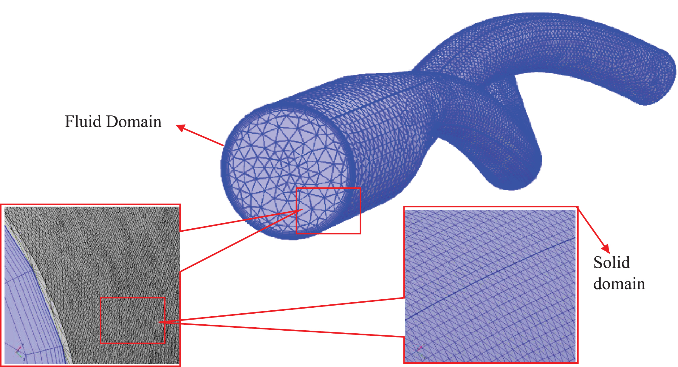
Computational fluid dynamics (CFD) was developed in the 1930 s as a branch of fluid mechanics to solve problems that are extremely complex for analytical methods. This method offers insights into hemodynamic factors, such as fluid velocity visualization and wall shear stress [19, 20]. In CFD, a fluid domain is usually divided into small tetrahedral or hexahedral elements called meshes (Fig. 4). Several governing equations are assigned to mesh elements, which further define boundary conditions to the neighboring elements in accordance with their equations of state. Therefore, a coupled system of elements is formed with an integrated view of the fluid dynamics of the system under consideration. The accuracy of the results obtained from this integration depends on the mesh quality, the imposed boundary conditions, and the algorithm implemented to compute the system of equations. Additionally, for a time-dependent study, the time step size between each iteration affects the solution accuracy. Hence, special care is required to develop a method for an accurate solution that matches the level of understanding of the investigated biological phenomenon [21].
Fig. 4
Mesh generated for the CFD evaluation of the ballet-type model. Tetrahedral mesh was generated for the fluid and solid domains, and hexahedral boundary layers were used near the boundary wall of fluid domain.
2.1Physical description
In this study, three representative patient specific, post-EVAR computed tomography (CT) images (Fig. 1a) were employed to model three-dimensional SG geometries. As depicted in Fig. 1b, the three planar and crosslimb SG configurations were ideally modeled, namely, top-down nonballet-type, top-down ballet-type, and bottom-up nonballet-type configurations. In top-down SG configuration, most of the device is deployed in the main body in the vicinity of renal artery and the limbs are extended to the iliac artery. While in the bottom-up configuration, some of the SG device is deployed in the main body, the limbs are deployed in aortic bifurcation, and the extra stent graft of the main body is extended to the proximal aorta until the below of the renal artery. The angle between the left and right iliac arteries (q CI) was defined as 42°. The dimensions of all three SG models, including the diameter of the infrarenal aortic artery (DMB), the diameter of the left and right common iliac arteries (CIA) (DCI), and the total length of the SG (L), were kept constant (Table 1) to perform a representative comparison. In all the models, the influence of graft roughness, graft limb tapering, and stent strut patterns were excluded.
Fig. 1a
CT images of the representative crosslimb EVAR patients.
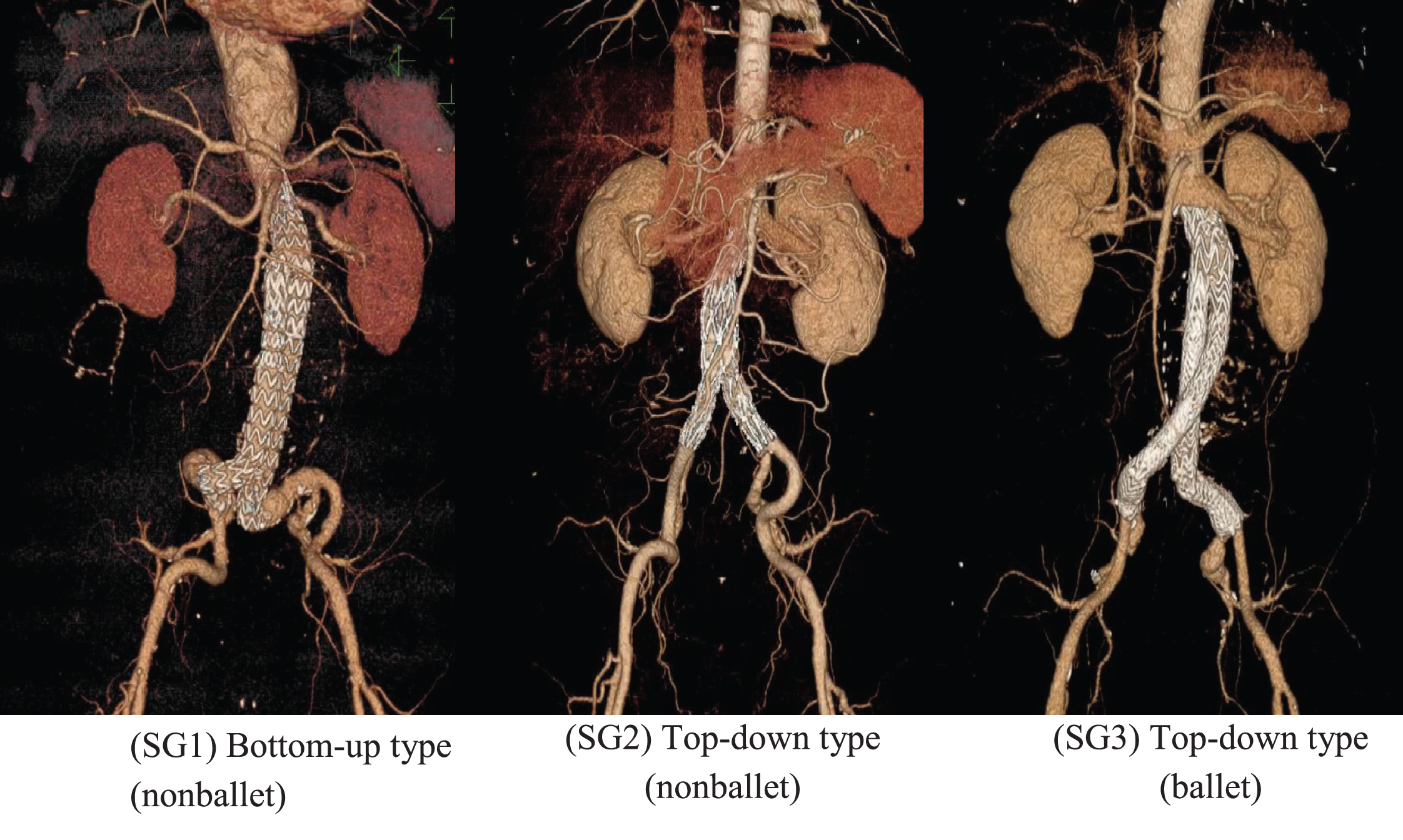
Fig. 1b
Ideally constructed three-dimensional models of patient specific geometries: bottom-up nonballet-type, top-down nonballet-type, top-down ballet-type.
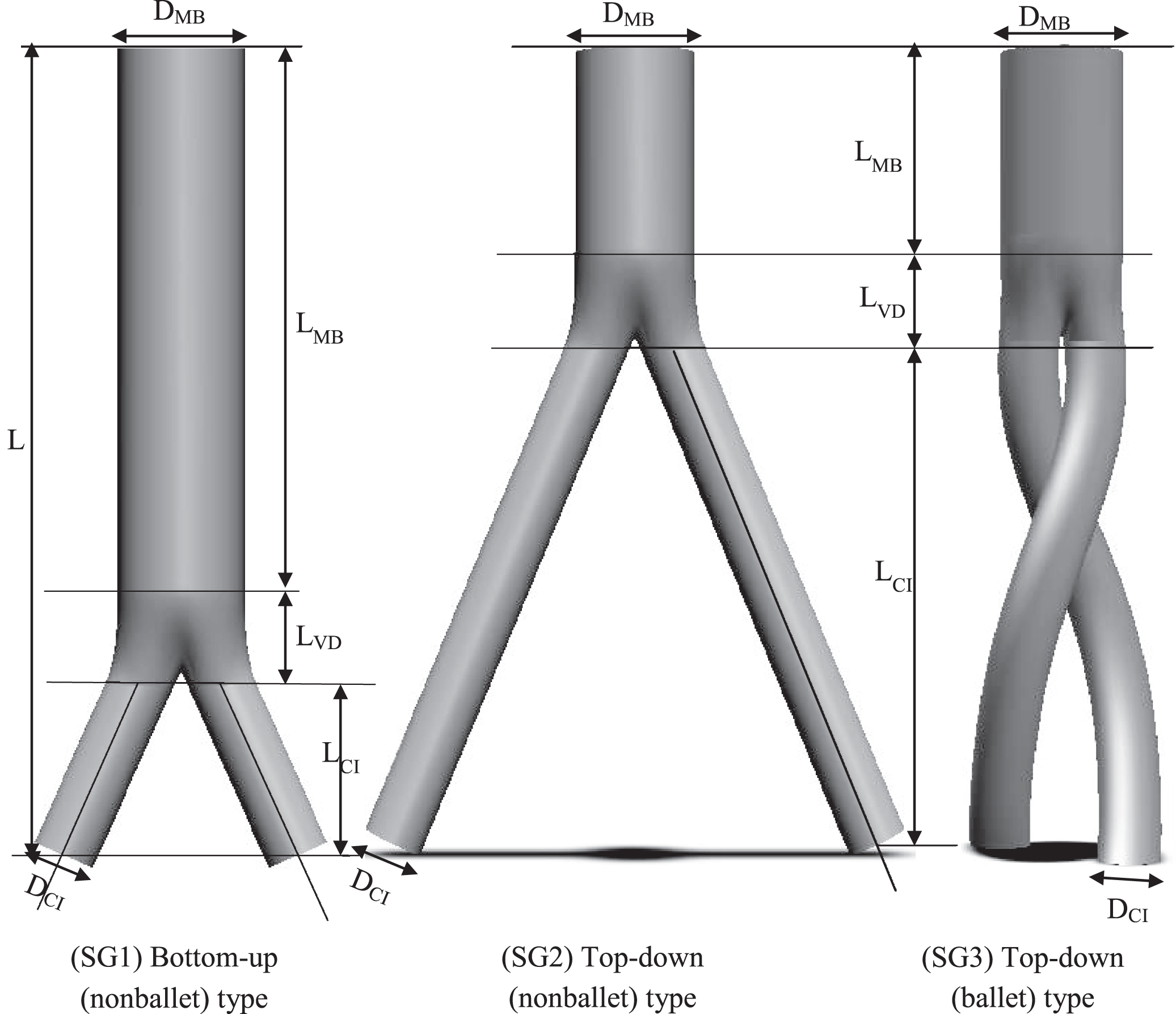
Table 1
Modeled dimensions of nonballet- and ballet-type models
| Parameters | Model 1 (a) | Model 2 (b) | Model 3 (c) |
| DMB | 26 | 26 | 26 |
| DCI | 13 | 13 | 13 |
| L | 170 | 170 | 170 |
| LMB | 110 | 40 | 40 |
| LCI | 40 | 110 | 110 |
| LVD | 20 | 20 | 20 |
2.2Mathematical model
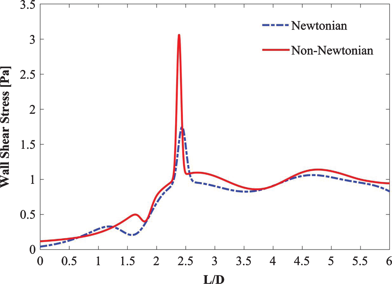
Blood can be treated as a homogenous and Newtonian fluid in vessels with hydraulic diameters exceeding approximately 0.5 mm [22–24]. Blood possesses variable viscous properties at low Reynolds numbers. In large arteries, for-example, in the aortic arch, blood is assumed to be a Newtonian fluid with a dynamic viscosity of 0.00345 Pa-s and density of 1050 kg/m3 [22, 25, 26]. Despite a number of supporting studies, several researchers claim that the assumption of blood as a Newtonian fluid underestimates the WSS values [27–29]. Non-Newtonian and Newtonian steady-state simulations were carried out to verify these assumptions as shown in Fig. 2. As inferred from the figure, the Newtonian flow assumption underestimates (with the maximum percentage difference of 6%) the WSS when compared with the non-Newtonian flow assumption. Moreover, the pulsatile cycle is dominated by the laminar flow in transient simulations. Though the Reynolds number at the peak systole is larger than the laminar range of flow and is followed by a flow declaration phase, however, these flow destabilization characteristics are temporary. They are preceded by an acceleration phase during systole and followed by a lengthy low-velocity diastole; both contribute to restabilizing the flow [30, 31]. Therefore, in this study, the laminar non-Newtonian velocity flow model was adopted for transient simulations with Reynolds number ranging from 158 to 3481.
Fig. 2
Comparison of steady Newtonian vs non-Newtonian flow.
Non-Newtonian pulsatile blood flow in the aorta was examined by using the Careau model of blood viscosity and fluid flow. This model is based on the three-dimensional incompressible Navier Stokes equation. The governing equations are described as follows:
(1)
(2)
where
(3)
where D and
(4)
where the infinite shear rate viscosity η∞ is 3.45×10⁻³ Pa.s, the zero shear rate η0 is 5.6×10⁻² Pa.s, n = 0.3568, and the relaxation time constant l is equivalent to 3.313 s. Table 2 summarizes all the blood flow properties used in the Eqs. 1–4.
Table 2
Physical properties of blood and SGs
| Material | ρ (kg/m3) | η∞ (Pa.s)) | η0 (Pa.s) | n | λ (s) | Ref. |
| Blood | 1050 | 3.45 × 10⁻³ | 0.607 | 0.3568 | 3.313 | [24, 25] |
| SG | Rigid | [23, 25] | ||||
Mills et al. [34] suggested that the um(t) inlet mean velocity and p(t) exit pressure waveforms corresponding to Re = 3348, are necessary to simulate pulsatile blood flow, especially in time-dependent analysis. In their study, velocity waveforms and blood pressure were examined in a series of patients at cardiac catheterization. The patients examined in this investigation were from a series of 23 and inspected during the course of routine diagnostic right or left cardiac catheterization at the National Heart Institute, Bethesda [34]. The ages of the patients ranged from 24 years to 60 years. According to the said study, the pressure in the abdominal aorta ranged from 70 mmHg to 110 mmHg. The inlet velocity peak systole, peak diastole, and exit pressure peak systole occurred at t = 0.4, 0.92, 0.5 s, respectively (Fig. 3). The Reynolds number (Re) is defined as follows:
(5)
![Velocity and pressure waveforms (Mills et al. [34]).](https://content.iospress.com:443/media/ch/2021/78-1/ch-78-1-ch200996/ch-78-ch200996-g003.jpg)
where u and μ signify the inlet mean velocity and blood viscosity, respectively.
Given that the present study is primarily focused on demonstrating the characteristics of blood flow within the three SG configurations, the effects of the cross pattern of stent wires were ignored, and the SG wall was assumed to be rigid. The SG walls were modelled by employing the rigid material model. The maximum Reynolds number in the present study is Re = 3481 based on the infrarenal inlet hydraulic diameter (DMB).
2.3Numerical scheme and boundary conditions
The finite element method-based commercial code COMSOL Multiphysics (V5.4) [35] was employed for the investigation of flow characteristics in the SG configurations. A time-dependent fluid flow study was simulated over a cardiac cycle for 1.1 s. The time step size was 0.01 s. Steady-state and transient simulations were conducted for each SG configuration. Keeping the initial velocity value zero caused no difference given that the simulation of multiple cardiac cycles rendered the initial condition of zero velocity negligible. Moreover, the velocity was specified as spatially uniform because variations in the inlet velocity profile negligibly affect the outlet velocity profiles [36]. A spatially uniform inlet velocity provides high estimates of shear stress magnitudes near the inlet boundary regions [31]. The convergence criterion for all the simulations was restricted to less than 1e-6. All computations were performed on an Intel(R) Xeon (R) CPU E5-2620 v3 with processors of 2.40 GHz and 64 GB RAM and 64-bit operating system. The post processing of hemodynamic indicators was done using MATLAB (vR2019b).
The inlet and outlet of the fluid domain were defined with the following time-dependent velocity and pressure formulas:
(6)
(7)
where d is the inlet diameter of the aorta, σnn represents the component of the traction parallel to the normal vector
(8)
2.4Evaluation parameters
The induced hemodynamic wall stresses and flow patterns based on the study of transient non-Newtonian pulsatile flow in three patient-specific AA SG geometries were evaluated to predict and compare their risks of SG migration and SG thrombosis. The differences in wall stresses, helical flow streamlines, graft displacement, velocity, and pressure contours of three SG configurations were also highlighted. Evaluation parameters such as helicity, time averaged wall shear stress (TAWSS), and oscillatory shear stress index (OSI) were evaluated using the mathematical expressions described in the following paragraphs.
Figure 9 depicts the absolute helicity values of all SG configurations during one cardiac cycle (Fig. 9). Absolute helicity is used to evaluate the intensity of helical flow throughout the SGs and is defined by using the following expression:
(9)
where ∇ × ν is the curl of velocity (vorticity) and n is the velocity vector.
The AWSS distribution at the critical sections of the throat and branches of the SG configurations at systolic, diastolic, and peak pressure conditions is illustrated in Fig. 10. The time-averaged WSS (TAWSS) is estimated by using the following expression:
(10)
where
(11)
(12)
where u is the velocity of the fluid and y is the distance from the surface.
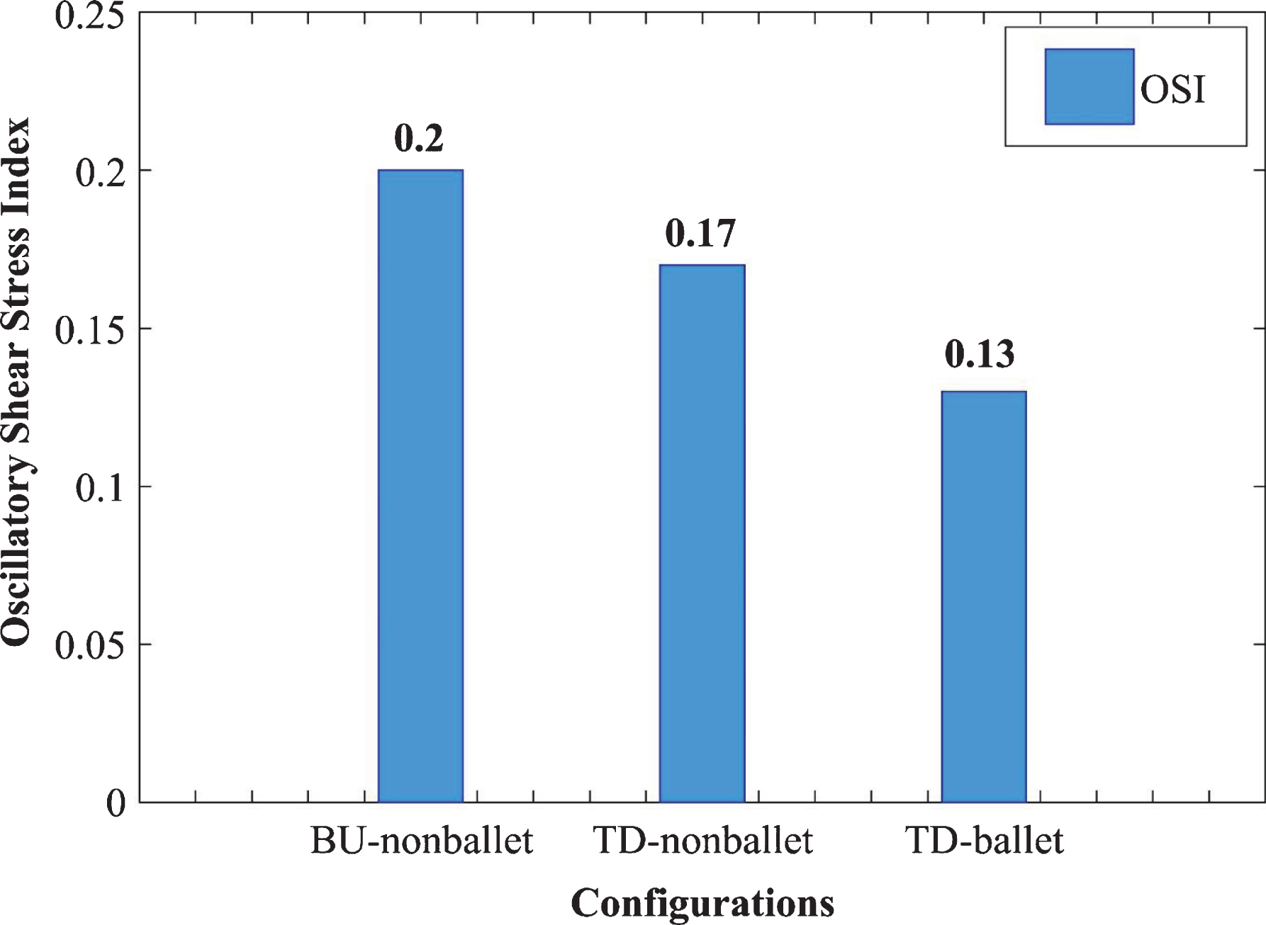
To quantify the directional change in WSS through time, the area-averaged OSI values for the three SG configurations were analyzed and compared using a bar graph (Fig. 11). The OSI values were calculated using the following expression [37];
(13)
Fig. 11
Area averaged OSI comparison of three SG configurations.
Where τ denotes the WSS vector and t signifies the time in the cardiac cycle of length T in seconds.
3Mesh independence
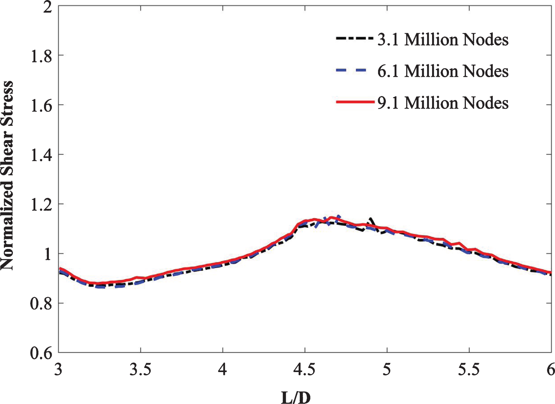
The accuracy of a computed solution considerably depends on the number of elements (mesh size) used per study. The accuracy of results improves by increasing the number of mesh elements at the expense of increasing computational costs. Therefore, an acceptable compromise between the mesh size and solution accuracy must be established. Thus, repeated computations are performed with various mesh sizes to obtain an optimal mesh size for the simulation of physical phenomena by utilizing the minimum computation cost without compromising the integrity of the computed solutions. This procedure is known as mesh independence or mesh refinement.
A finite element free-tetrahedral mesh was used for the fluid and solid domains to discretize the computational domain as depicted in Fig. 4. The three idealized graft configurations were imported into COMSOL Multiphysics (v5.4) [35] for tetrahedral meshing with hexahedral boundary layers. Mesh independence for each configuration was performed by applying steady-state boundary conditions and non-Newtonian Careau blood viscosity model properties. For the top-down ballet-type graft configuration, the predicted values of outlet velocity profiles (Table 3) and WSS (Fig. 5) were plotted and monitored for three different mesh sizes: M1, M2, and M3. Comparing the outlet velocity results revealed increasing the mesh size from M1 to M2 resulted in a maximum percentage difference of 0.02%. The average percentage differences between the values of WSS obtained by utilizing meshes M1, M2, and M3 were 1.3% (M1–M2) and 0.6% (M1–M3). Therefore, the M1 mesh with 3.1 million nodes was adopted for subsequent simulations to obtain an accurate solution at the expense of minimal computational resources.
Table 3
Details of the mesh independence study
| Mesh | Total number of nodes | Outlet velocity (m/s) | % Difference |
| M1 | 3.1 million | 0.9113 | – |
| M2 | 6.1 million | 0.9111 | 0.02% |
| M3 | 9.1 million | 0.9110 | 0.03% |
Fig. 5
Mesh independence study.
4Model validation
The employed computational model was validated on the basis of the experimental study of Shemer et al. [38] at a Reynolds number of 4,000. The authors investigated pulsatile turbulent fluid flow at the inlet of a pipe and applied an oscillatory pressure at the pipe outlet. Afterward, they studied the flow properties throughout the pipe and measured the velocity at the pipe exit. Given that the properties of this research are similar to those of the present study, the conditions of the experiment by Shemer et al. [38] were regenerated numerically, and the obtained results were compared with the corresponding experimental values. The computed velocity values were normalized with the maximum velocity magnitude. Figure 6 demonstrates that the nondimensional velocity results are in accordance with the experimental data and yielded a maximum deviation of 3%, which is within an acceptable range.
Fig. 6
Comparison of the normalized axial velocity in a pipe between the present results and those of Shemer et al. [38] at Re = 4,000.
![Comparison of the normalized axial velocity in a pipe between the present results and those of Shemer et al. [38] at Re = 4,000.](https://content.iospress.com:443/media/ch/2021/78-1/ch-78-1-ch200996/ch-78-ch200996-g006.jpg)
5Results
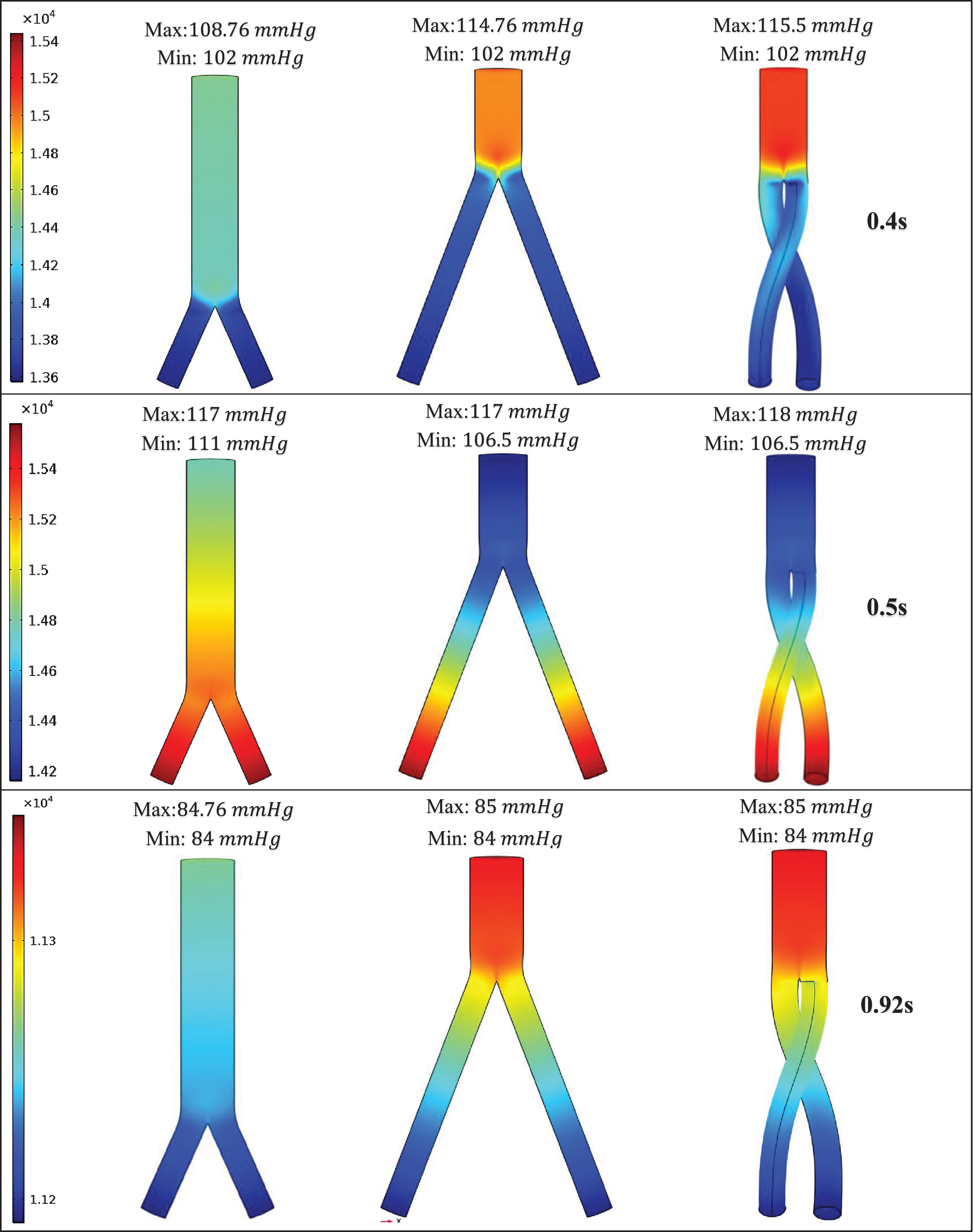
In this study, the blood flow patterns and induced hemodynamic wall stresses in three ideally designed patient-specific AA SG configurations were comparatively analyzed. The investigated SG configurations included a top-down nonballet-type, a top-down ballet-type, and a bottom-up nonballet-type model. Blood flow dynamics were examined at three stages of a pulsatile cycle: systole (maximum velocity) (0.4 s), peak pressure (0.5 s), and diastole (0.92 s). The results are analyzed in terms of WSS, flow streamlines, helicity, velocity, and pressure contours.
The flow streamlines were plotted at the three time points (systole [0.4 s], peak pressure [0.5 s] and diastole [0.92 s]) to visualize the blood flow pattern and distribution in the three aortic SG configurations as shown in Fig. 7. The flow streamlines for the systolic (0.4 s) condition or at maximum velocity (Fig. 7a) demonstrate that the velocity magnitude was smallest in the bottom-up nonballet-type SG configuration. While the highest value of velocity was observed in the top-down ballet-type SG configuration followed by that in the top-down nonballet-type SG configuration.
Fig. 7a
Mean velocity streamline plots of the (SG1) bottom-up nonballet-type model (SG2) top-down nonballet-type model (SG3) top-down ballet-type model under systolic conditions (0.4 s).
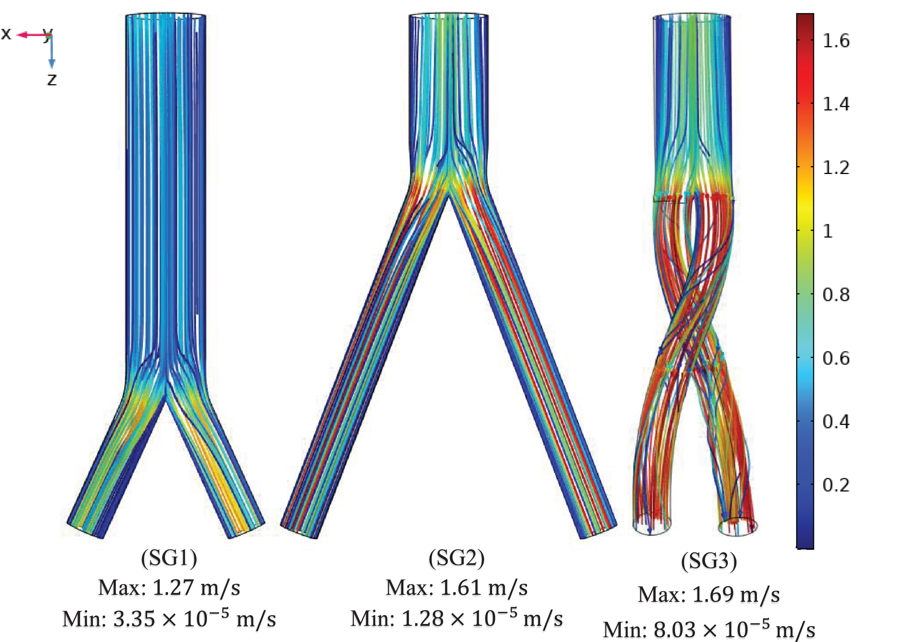
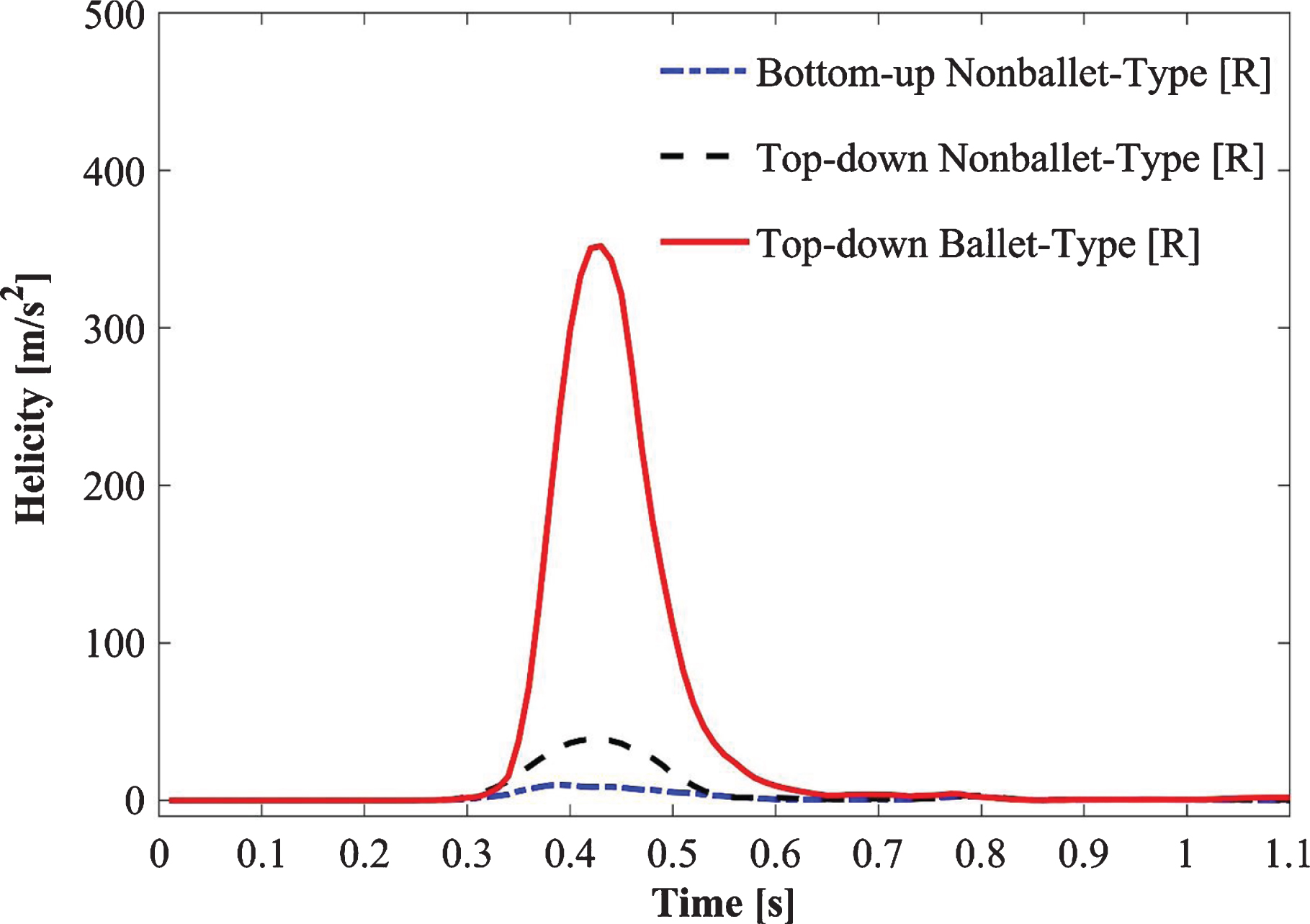
Figure 9 depicts the absolute helicity values of all SG configurations during one cardiac cycle (Fig. 9). For all SG configurations, a peak helicity value was detected at the time point 0.4 s >t>0.5 s. The ballet-type model showed the maximum magnitude of helicity, whereas negligible helicity was observed for the bottom-up nonballet-type SG. Compared with those of the bottom-up and top-down nonballet-type models, the helicity values of the ballet-type model have reached a maximum of 95% and 84%, respectively. The helicity values ranged from 0.01-418 m/s2 as shown in the Fig. 9.
The AWSS distribution at the critical sections of the throat and branches of the SG configurations at systolic, diastolic, and peak pressure conditions is illustrated in Fig. 10. Figure 10 (a, b) demonstrates that the trend of the AWSS distribution is analogous across the right and left iliac arterial SGs of different configurations. Depending on the flow mean velocity, the TAWSS values were plotted in the order of systolic, peak pressure, and diastolic stage of the cardiac cycle for all the stent configurations as shown in Fig. 10 (a, b). The AWSS for the nonballet SG models exhibited a peak value along the wall of the SGs and declined to considerably reduced stabilized values after the bifurcation region. The peak AWSS values of different SG models decreased in the order of top-down nonballet-type, bottom-up nonballet-type, and top-down ballet-type models. However, the ballet-type model featured the highest overall AWSS among all SG configurations, and its WSS values were uniformly distributed. The AWSS values of the ballet-type model were 21% and 38% higher than those of the top-down and bottom-up nonballet type models, respectively. The AWSS values ranged from 0.2-24 Pa, as shown in Fig. 10.
Fig. 10a
AWSS for the right iliac arterial SG at systole (0.4 s), peak pressure (0.5 s) and diastole (0.92 s).
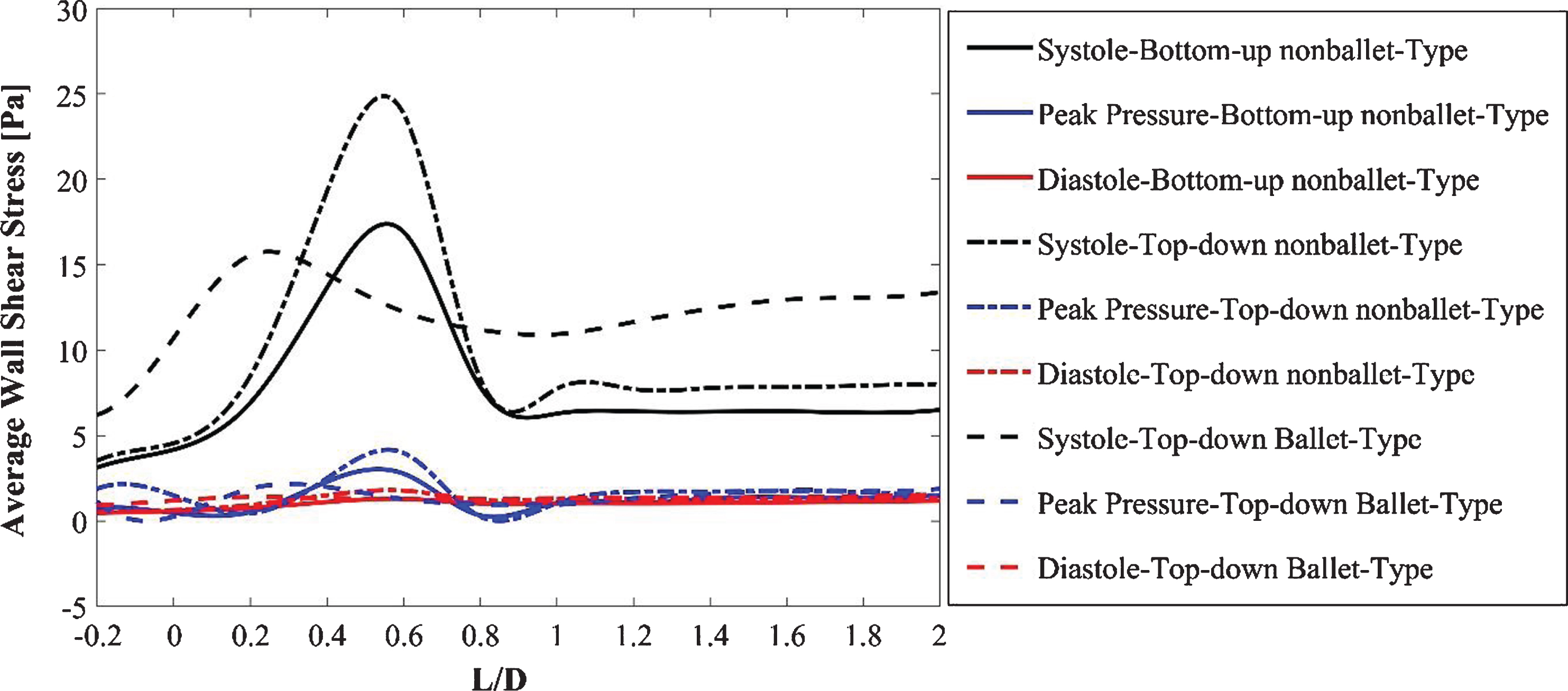
Fig. 10b
AWSS for the left iliac arterial stent graft at systole (0.4 s), peak pressure (0.5 s) and diastole (0.92 s).
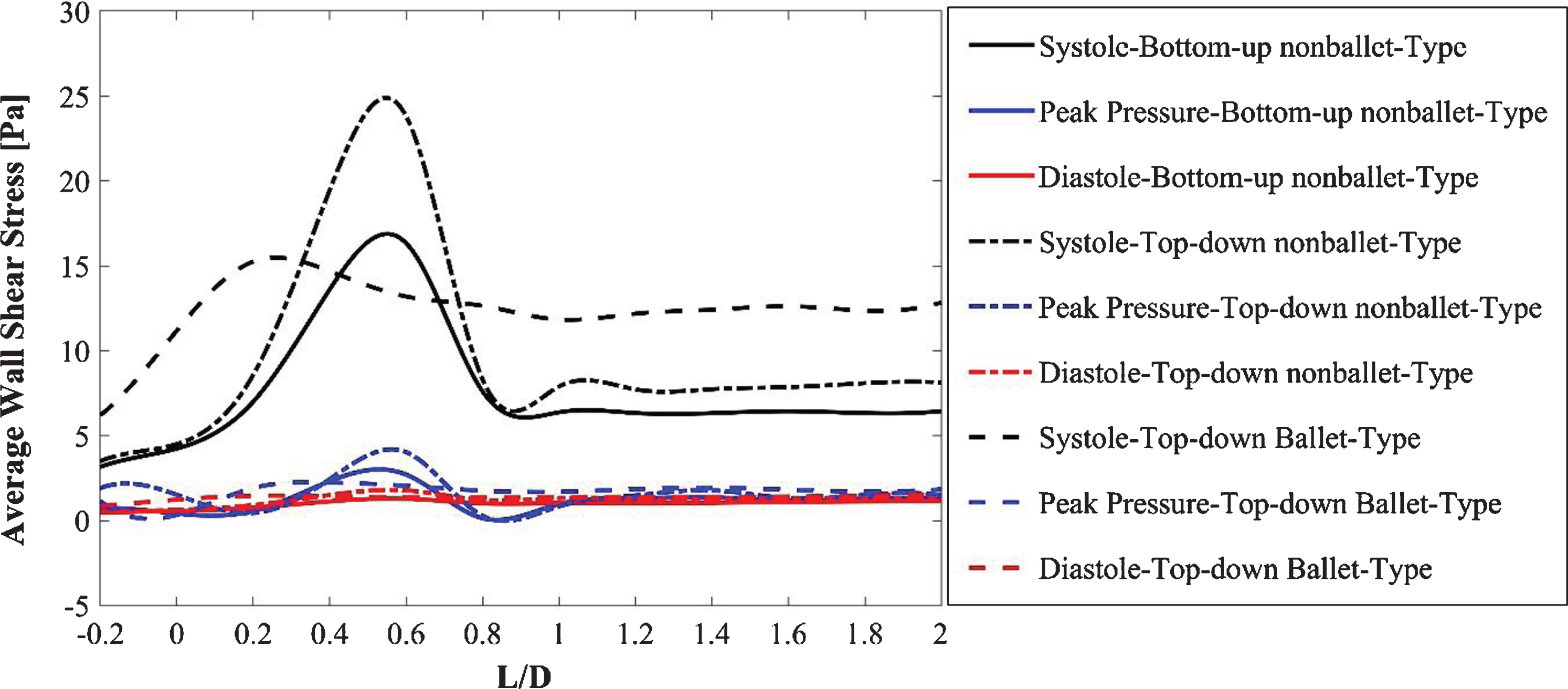
To quantify the directional change in WSS through time, the area-averaged OSI values for the three SG configurations were analyzed and compared using a bar graph (Fig. 11). The 0 magnitude of OSI represents unidirectional flow with no change in the WSS direction over the time period T, and a value of 0.5 indicates an intensively oscillating flow. A larger OSI demonstrates the higher risk of local thrombosis [39]. The OSI results of the ballet type model showed approximately 23% lesser values than that of the top-down nonballet-type model. The OSI values ranged from 0.13-0.2, as shown in Fig. 11.
Figure 12 displays the total pressure distributions across all three SG configurations under systole (0.4 s), peak pressure (0.5 s), and diastole (0.92 s) conditions. At all time points of the cardiac cycle, the bottom-up nonballet type model featured the lowest pressure among all three SG configurations. The pressure distributions in top-down type models were similar in terms of the gradient. However, the ballet type model showed a maximum magnitude of pressure under systolic and peak pressure conditions. The largest pressure gradients were observed under the peak systole and peak pressure conditions. The maximum pressure of the ballet-type model is 5.83% and 0.64% higher than that of the low- and top-down nonballet-type models, respectively, at the peak systolic instance. The maximum pressure of the ballet-type model is 0.85% higher than that of the bottom-up and top-down nonballet-type models at the peak pressure instance.
Fig. 12
Pressure distribution under systolic (0.4 s), peak pressure (0.5 s), and diastolic (0.92 s) conditions.
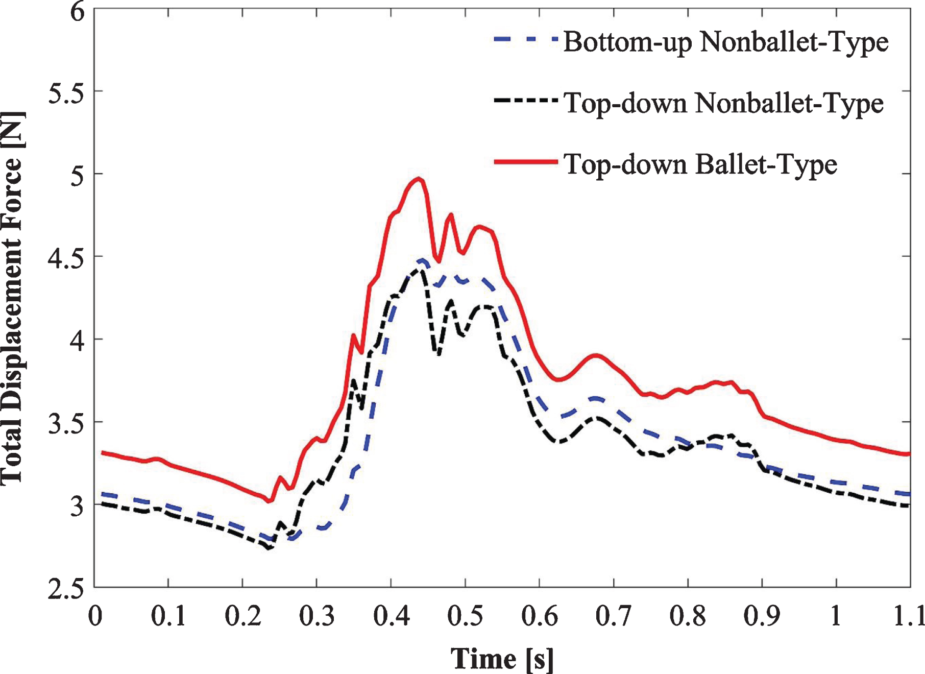
The total displacement forces are calculated for the three SGs as depicted in Fig. 13. The displacement forces acting on the SG walls include: the normal force exerted by the blood pressure and the WSS induced tangential force. The summation of these force components yields the total displacement force which is helpful to forecast the SG migration [31, 40–42]. Figure 13 demonstrates that in accordance with the pressure waveforms, the displacement force is maximum at the optimal value of pressure in the cardiac cycle (Fig. 3). Ballet-type model displacement forces are 40% higher than the bottom-up nonballet-type model and 9.6 % higher than the top-down nonballet-type model. The total displacement force observed in these SGs was 40% and 9.6% lower than the ballet-type (non-planar) SG. In all the SG configurations, the direction of the total displacement force was noted to be in the upward direction. The total displacement force values ranged from 2.75-4.97 N, as shown in Fig. 13.
Fig. 13
Variation of total displacement forces over time for bottom-up nonballet-type model, top-down nonballet-type model and top-down ballet-type model.
6Discussion
Several researchers examined the effects of in vivo crosslimb EVAR. One such clinical in vivo study compared the conventional and crosslimb EVAR techniques in 27 patients by employing the Kaplan-Meier method. The comparison showed an insignificant difference between the two techniques and rendered it safe to use on AAA patients [43]. Yagihashi et al. [44] reported similar results in another investigation based on the early and midterm results of crosslimb and conventional EVAR techniques. The researchers considered EVAR technique to be safe for the treatment of all AAA cases including the severely splayed iliac angulation [44].
6.1Fluid flow physiognomies
In all the SG configurations, the flow velocity increases as the fluid enters the branched sections to conserve momentum. The helicity of the ballet type model promotes helical flow patterns as the blood flows downstream of the branches (Fig. 7a). Compared with those observed under systolic and diastolic conditions, complex blood flow patterns were observed under peak pressure conditions (Fig. 7b) in all three SG configurations. These flow patterns can be escribed to the reduction in the fluid inlet mean velocity and reverse flow at this instance of the systolic cycle. Therefore, a negative velocity gradient, which promotes the formation of two lateral vortices (flow recirculation) near the entrance of the stent, is generated. These lateral vortices are highly prominent in the nonballet and ballet type models. The lateral vortices of the stent entrance disappeared at the diastole stage (0.92 s), and the flow was in a steady state as depicted in Fig. 7c.
Fig. 7b
Mean velocity streamline plots of the (SG1) bottom-up nonballet-type model (SG2) top-down nonballet-type model (SG3) top-down ballet-type model under peak pressure conditions (0.5 s).

Fig. 7c
Mean velocity streamline plots of the (SG1) bottom-up nonballet-type model (SG2) top-down nonballet-type model (SG3) top-down ballet-type model under diastolic conditions (0.92 s).
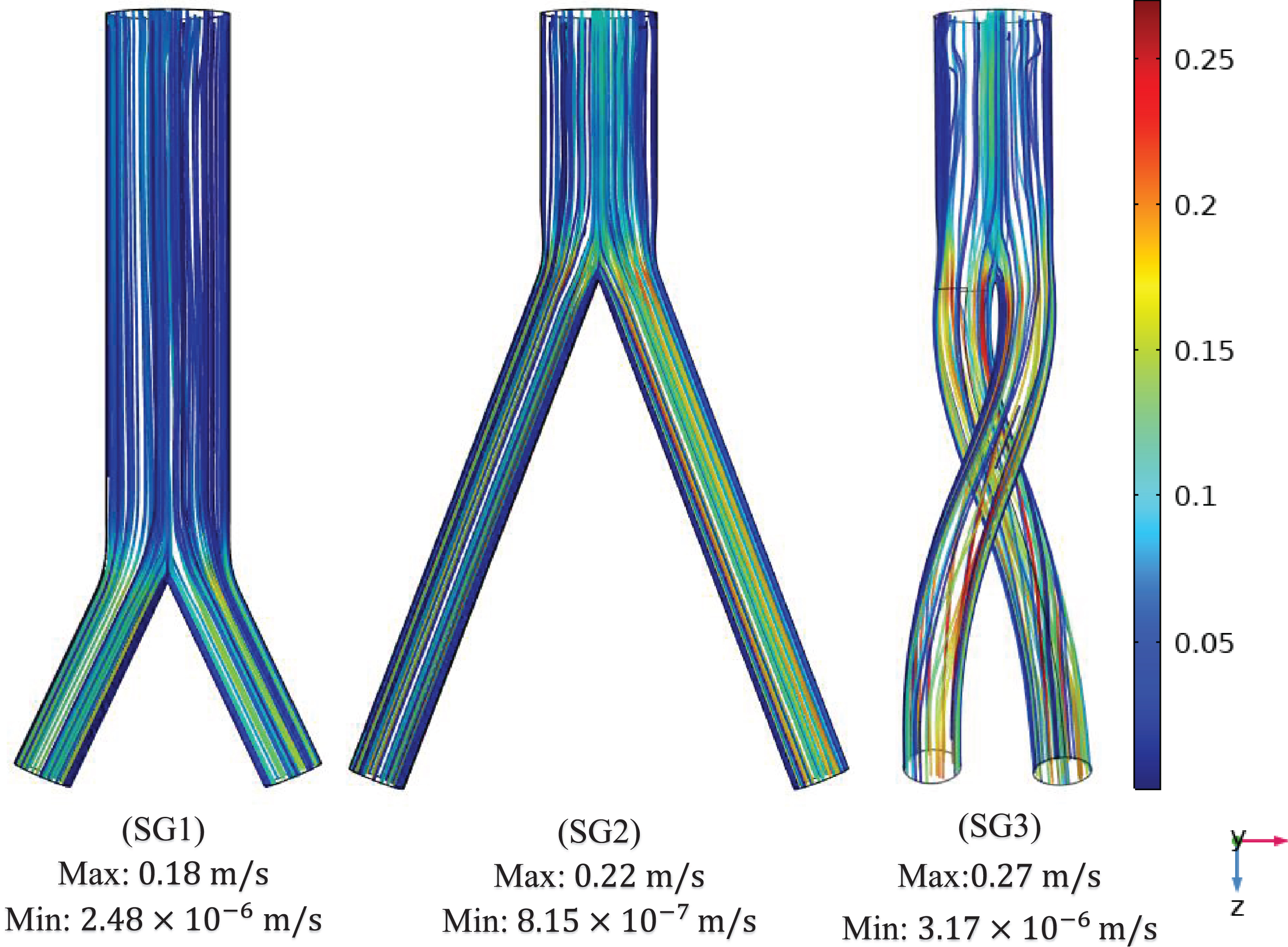
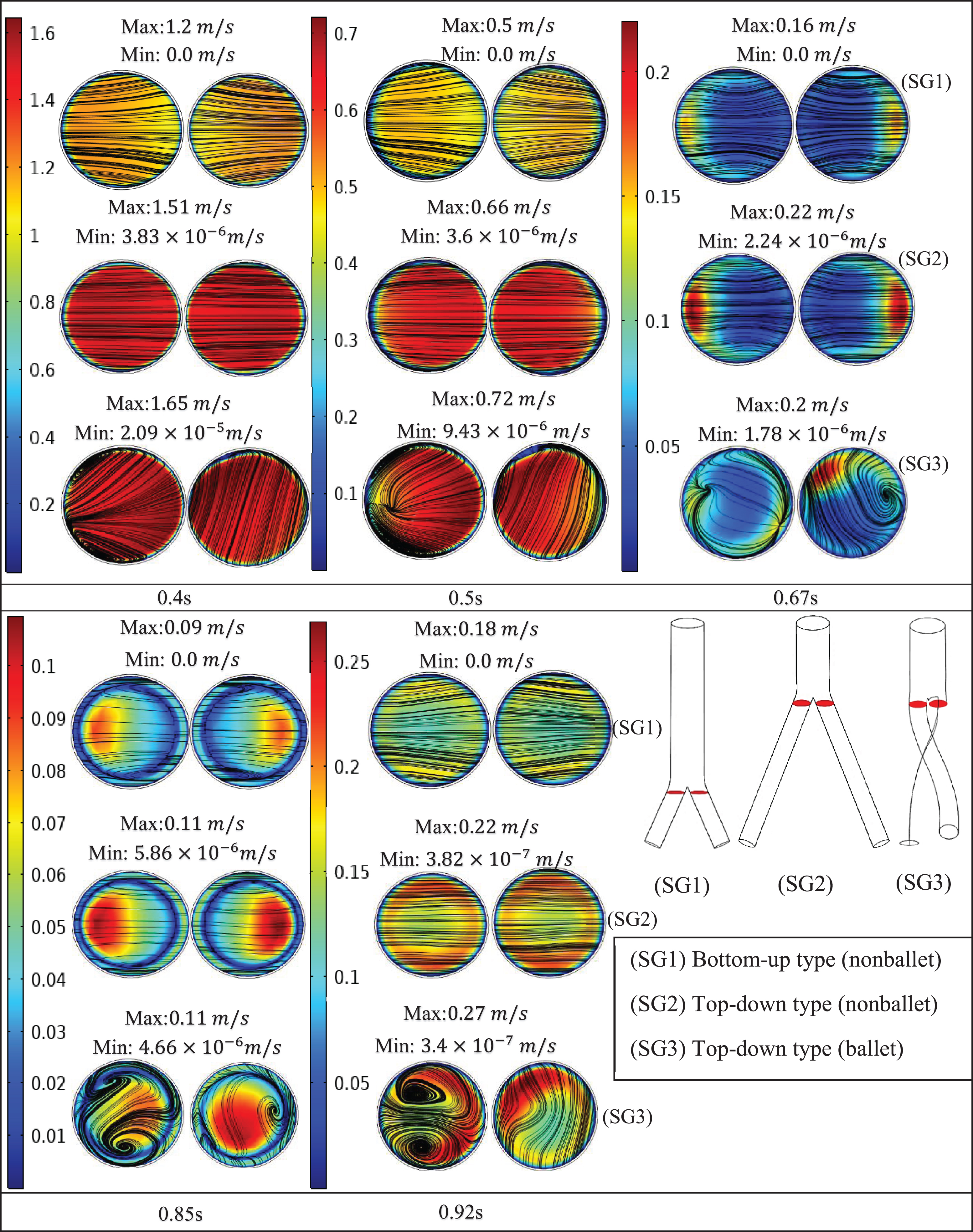
Figure 8 presents the velocity contours and streamlines along three cross-sections (throat, branch intersection, and early branches) of the three SG configurations at all the studied stages of the cardiac cycle. Two pairs of symmetrical vortices and one pair of helical vortices can be observed at the throat of the top-down nonballet- type and top-down ballet-type SGs, at t = 0.67 s (Fig. 8a). These vortices intensified at t = 0.85 s. Additionally, the bottom-up nonballet-type model also demonstrated the formation of two pairs of symmetrical vortices at this instance. At the branch intersections and early branch cross-sections (Fig. 8b, c), the flow distribution in the branches was uniform without vortices at all the time points for the nonballet-type SG models. However, the helical vortices at the branch intersection and early branch cross-sections of the ballet type SG configuration presented a flow helicity at t≥0.67 s. Helicity can be explained as the flow reaching the branched sections and the streamlines converging toward the interior interface of branches. Meanwhile, under the action of centrifugal forces and high-pressure magnitudes, the flow swirls generate backflow at late systole (0.67 s). These flow swirls lead to the generation of secondary flow vortices at the later time points (0.85 s) (Fig. 8a, b, c).
Fig. 8a
Velocity magnitude and streamline contour plots at throat representing systole (0.4 s), peak pressure (0.5 s), late systole (0.67 s), early diastole (0.85 s) and diastole (0.92 s).
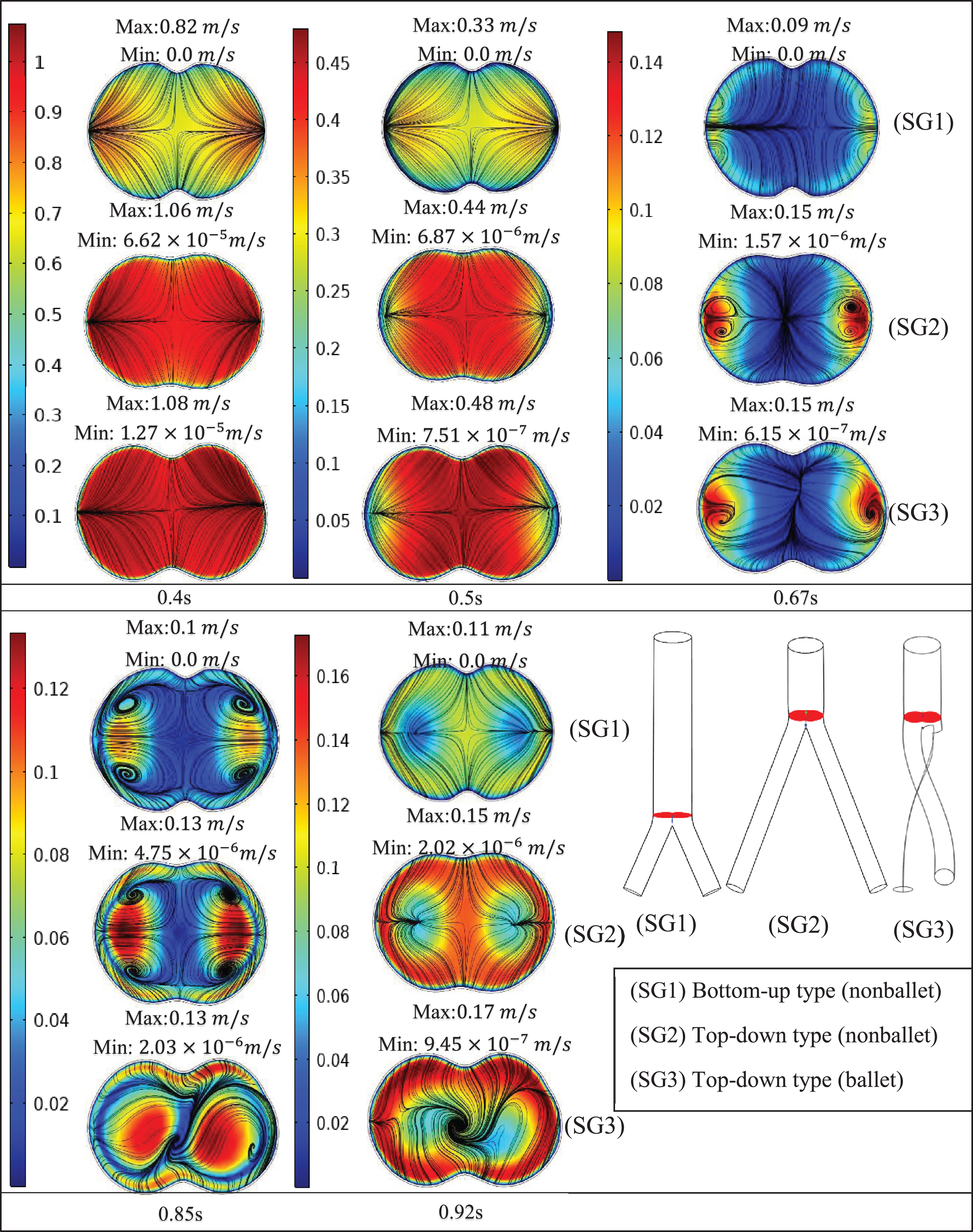
Fig. 8b
Velocity magnitude and streamline contour plots at branch intersection representing systole (0.4 s), peak pressure (0.5 s), late systole (0.67 s), early diastole (0.85 s) and diastole (0.92 s).
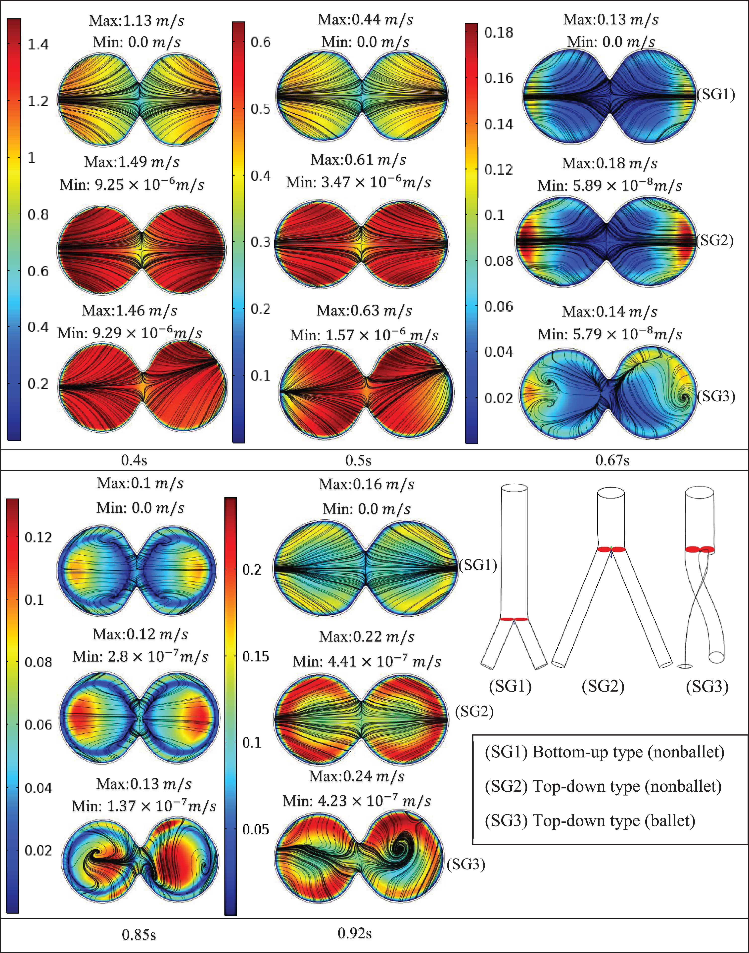
Fig. 8c
Velocity magnitude and streamline contour plots at early branches representing systole (0.4 s), peak pressure (0.5 s), late systole (0.67 s), early diastole (0.85 s) and diastole (0.92 s).
6.2Helicity
Blood flow helicity in the human vascular system demonstrates multiple beneficial effects [45–53]. Morbiducci et al. [50] demonstrated that efficient perfusion can be achieved in the human vascular system with the help of helical flow form. Flow helicity inhibits excessive energy dissipation and thereby stabilizes blood flow [51]. Helical flow reduces flow separation within the carotid bifurcation and, thus prevents atheroprone hemodynamics [52]. Moreover, helical flow displays important biological features; for example, it inhibits atherosclerosis and thrombosis formation by disrupting the transport of materials, such as atherogenic lipids, thereby decreasing platelet adhesion on walls of arteries [45, 53–55].
The high magnitude of helicity in the ballet-type configuration, which signifies good helical flow patterns, is reflected by the large magnitude of WSS for the ballet-type model throughout the limbs. High average WSS (AWSS) in the ballet-type model resulted from the high centrifugal forces of helical flow. Furthermore, as the diastole of the physiologic inlet velocity profile approached, it dampened the helical flow in the later periods of the cycle. At the outlet of the graft limb, the effective helical flow in all the configurations occurred for only 0.3 s (from 0.3 s ≤t≤0.6 s) as shown in Fig. 9a, b. The short duration of effective helical flow may be ascribed to the high dependence of helicity on velocity; given this dependence, low magnitudes of velocities resulted in near-zero helicity at the outlets [31]. Moreover, the high helicity values in the left graft outlets for top-down type models are likely inherited from the natural posteriority of the left CIA [56]. Past studies suggested that sustained helical flow contributes to the reduction in graft-limb occlusion stimulated by thrombosis formation within the SG [45, 54, 55, 57, 58]; therefore the cross-limb configuration may help in increasing resistance to thrombosis.
Fig. 9a
Absolute helicity variation at the left outlet of the iliac branch of SG configurations.
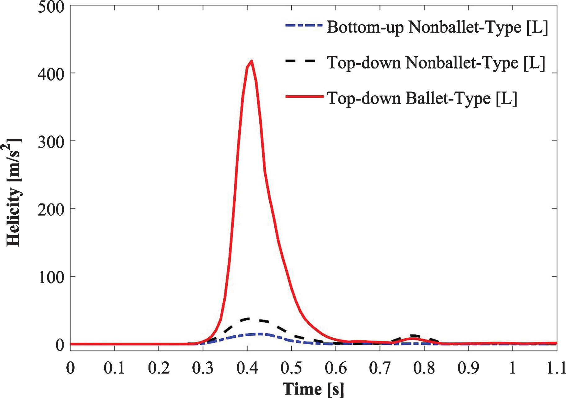
Fig. 9b
Absolute helicity variation at the right outlet of the iliac branch of SG configurations.
6.3Average Wall Shear Stress (AWSS)
The EVAR effect on vascular wall stresses is a postprocedural complication. The spatial distribution of WSS plays an important role in the localization and development of graft thrombosis and predicting rupture risk [31, 47, 59]. The concentration of vascular stress is influenced by various factors, including the location of the aneurysm, asymmetry, and geometric irregularities [59]. The regions of the SG walls, which experience high unidirectional WSS, show high resistance to flow-related thrombosis, whereas oscillatory WSS contributes to flow-related thrombosis [37, 39]. Furthermore, helical flow reduces thrombosis risk by enhancing the WSS due to the presence of centripetal and centrifugal forces [47, 60]. Centrifugal force diminishes deposit accumulation and flow separation and stagnation, whereas centripetal force accelerates mass transport.
The peak AWSS values of the SG models are correlated with the sudden change in the orientation of the branches and accelerating flow velocity as the fluid enters the branches of the models as discussed in the previous section (Figs. 7 and 8). In addition, the angle at which the branches are oriented is an important factor that determines the differences in the AWSS values of the three models [61]. Moreover, the differences in flow patterns in the suprarenal and infrarenal abdominal aorta of humans cause blood flow reversal, which can be observed in early diastole in the infrarenal aortas of young, healthy humans; this reversal causes the flow waveform to become a triphasic (forward in systole reverse in early diastole forward in late diastole) waveform over the cardiac cycle (Fig. 3) [62].
Shek et al. [31] analyzed the fluid flow characteristics in a patient-specific crosslimb EVAR configuration by assuming Newtonian blood flow. Their results showed that the helical flow generated in the crosslimb EVAR technique offers a major advantage in increasing the resistance to flow-related thrombosis. The AWSS values of the ballet-type model were 21% and 38% higher than those of the top-down and bottom-up nonballet type models, respectively (Fig. 10a, b). Therefore, the ballet-type configuration may reduce graft thrombosis by increasing the WSS. Moreover, the similar trends shown by the transient AWSS values for all configurations suggest that the identical main body of all the SGs may have accounted for the regions, i.e., bifurcations, with the highest WSS magnitudes.
The absolute value of WSS is used to analyze the spatial variation of shear stress along walls, whereas oscillatory shear stress index (OSI) values are used for characterizing the temporal behavior of WSS. The 0 magnitude of OSI represents unidirectional flow with no change in the WSS direction over the time period T, and a value of 0.5 indicates an intensively oscillating flow. A larger OSI demonstrates the higher risk of local thrombosis [39]. In this report, the area-averaged OSI values for the three SG configurations were analyzed and compared using a bar graph (Fig. 11). As the results show that the OSI of the ballet type model is approximately 23% lower than that of the top-down nonballet-type model. Therefore, balleting (crosslimb) the SG limbs reduces the risk of graft thrombosis relative to nonballeting.
6.4Pressure distribution
As the pressure distributions in the top-down type models were similar in terms of pressure gradients, this similarity suggests that the identical main body of top-down type SGs must have accounted for regions, i.e., bifurcations, hence causing similar gradient trends in top-down type models. However, maximum pressure gradient was observed in ballet-type configuration. The change in wall pressure is time-dependent, and the pulsatile nature of the flow causes the oscillation of wall pressure gradients. The sequential accelerations and decelerations of the flow largely affect the pressure distribution at the wall during pulsatile flow (Fig. 12). The pressure distribution across all the SG configurations at systolic, and peak pressure conditions represents the reverse flow as discussed in Section 6.1. The high-pressure gradients on the walls of the ballet-type model suggest that pressure forces for this model are higher than those for other SG configurations. This condition may lead to fatigue and may thus cause the failure of the SG over the long term.
6.5Total displacement forces
Graft migration is one of the major cause of graft failure and often requires reintervention [16, 63]. It is the slippage of SG to a distal location and is associated with the SG oversizing and aortic neck altercations. Despite the introduction of proximal active fixation devices i.e. hooks, barbs, and proximal stents in latest generations of SGs to provide the uniaxial fixation strengths [64, 65], the graft migration risk still remains. Literature studies demonstrate that the SG displacement forces, the root cause of graft migration, usually tend to augment with the higher blood pressure and non-planar SG configurations [36, 41, 42, 66, 67]. Liu et al. [33] employed the crosslimb strategy to construct various ideal SG configurations with different torsion angles and performed computational and experimental studies to analyze the effect of changing the torsion angles of crossed iliac limbs on the hemodynamics of blood flow and predicted graft migration, and graft thrombosis risks. Their results suggest that an increase in torsion angle increases the risk of SG migration.
The displacement forces of ballet type configuration are 40% and 9.6% higher than the bottom-up nonballet- and top-down nonballet- type configurations, respectively. The direction of the displacement forces was noted to be in upward direction. Though the migration of the SGs in the upward direction is a rare phenomenon, however, multiple reports support this observation [68–70]. However, it is worth mentioning that these displacements forces tend to be lower in magnitude than the displacement resistance offered by active fixations e.g. barbs, hooks, radial forces, and columnar strength [64]. The present results are in agreement with experimental studies reported by Corbett et al. [71] and Liu et al. [33]. These reports demonstrated that the increase in out-of-planarity of SGs is directly related to increment in axial migration forces. Similar trends were noted in this study for the case of bottom-up and top-down nonballet-type (planar) models. Therefore, the crosslimb strategy should be carefully employed in the surgical treatment of AAA. Hence, it can be concluded that the ballet-type SG model is more prone to failure compared to other SG configurations due to different forms of structural fatigue.
7Conclusion
A comparative analysis of the induced hemodynamic wall stress and flow patterns was performed based on the study of transient non-Newtonian pulsatile flow in three ideally designed patient-specific AA SG geometries. A time-dependent fluid flow study was simulated over a cardiac cycle of 1.1 s. The three SG configurations, namely, the top-down nonballet-type, top-down ballet-type, and bottom-up nonballet-type models were evaluated to highlight the differences in wall stresses, flow streamlines, velocity, and pressure contours. The study findings are summarized as follows:
• The generation of helical flow in the ballet-type configuration preserves blood flow and thereby makes the utilization of the ballet configuration as safe as that of conventional configurations.
• The crosslimb configuration may reduce the tendency of bio-cell accumulation (i.e., RBDC, platelet, LDL particles, and any thrombotic structure, etc.) given that the helicity of the ballet-type model is 95% and 84% higher than that of the bottom-up (nonballet) and top-down (nonballet) type SGs, respectively.
• The OSI of the ballet-type model is 23 % less than that of the top-down nonballet-type model. This condition also indicates that the technique of balleting (crosslimb) the SG limbs may reduce the risk of bio-cell accumulation i.e., RBDC, platelet, LDL particles, and any thrombotic structure, etc.
• The pressure magnitude for the ballet-type model is 5.83% and 0.64% larger than that for the low- and top-down nonballet-type models, respectively. While the displacement forces of the Ballet-type model are 40% and 9.6% higher than the bottom-up and top-down nonballet-type models, respectively. This characteristic may cause high fatigue in the ballet-type model and thereby lead to failure over the long term.
Acknowledgments
This study was supported by the National Research Foundation of Korea grant funded by the Korean government (MSIP) (No. 2020R1A2B5B02002512, 2020R1A4A1018652).
Conflict of interest
The authors have no conflict of interest to report.
References
[1] | Benjamin EJ , Muntner P , Alonso A , Bittencourt MS , Callaway CW , Carson AP , et al. Heart Disease and Stroke Statistics-2019 Update: A Report From the American Heart Association. Circulation. (2019) ;139: (10):e56–66. 10.1161/CIR.0000000000000659. |
[2] | Amiri MH , Keshavarzi A , Karimipour A , Bahiraei M , Goodarzi M , Esfahani JA . A 3-D numerical simulation of non-Newtonian blood flow through femoral artery bifurcation with a moderate arteriosclerosis: investigating Newtonian/non-Newtonian flow and its effects on elastic vessel walls. Heat Mass Transf und Stoffuebertragung. (2019) ; 10.1007/s00231-019-02583-4. |
[3] | British Heart Foundation. Heart & Circulatory Disease Statistics 2019 - Cardiovascular Disease Statistics - BHF [homepage on the Internet]. 2019 [cited 2019 Oct 21]. |
[4] | Khanafer KM , Bull JL , Berguer R . Fluid-structure interaction of turbulent pulsatile flow within a flexible wall axisymmetric aortic aneurysm model. Eur J Mech B/Fluids.(2009) ;28: (1):88–102. 10.1016/j.euromechflu.2007.12.003. |
[5] | Gillum RF . Epidemiology of aortic aneurysm in the United States. J Clin Epidemiol. (1995) 48: (11):1289–98. 10.1016/0895-4356(95)00045-3. |
[6] | Al-Omran M , Verma S , Lindsay TF , Weisel RD , Sternbach Y . Clinical Decision Making for Endovascular Repair of Abdominal Aortic Aneurysm CLINICIAN UPDATE e517. Circulation. (2004) 110: :517–23. |
[7] | Katzen BT , Dake MD , MacLean AA , Wang DS . Endovascular repair of abdominal and thoracic aortic aneurysms. Vol. 112, Circulation. 2005. pp. 1663-75. 10.1161/CIRCULATIONAHA.105.541284. |
[8] | Swerdlow NJ , Wu WW , Schermerhorn ML . Open and Endovascular Management of Aortic Aneurysms. Circ Res.(2019) ;124: (4):647–61. 10.1161/CIRCRESAHA.118.313186. |
[9] | Ogawa Y , Watkins AC , Lingala B , Nathan I , Chiu P , Iwakoshi S , et al. Improved midterm outcomes after endovascular repair of nontraumatic descending thoracic aortic rupture compared with open surgery. J Thorac Cardiovasc Surg. 2020;10.1016/j.jtcvs.2019.10.156. |
[10] | Huu A Le , Green SY , Coselli JS . Thoracoabdominal Aortic Aneurysm Repair: From an Era of Revolution to an Era of Evolution [homepage on the Internet]. Vol. 31, Seminars in Thoracic and Cardiovascular Surgery. 2019 [cited 2020 Feb 17]. pp. 703-7. 10.1053/j.semtcvs.2019.05.039. |
[11] | A Population-Based Study of Abdominal Aortic Aneurysm Treatment in Finland 2000 to 2014. Circulation. (2017) ; (136):1726–34. 10.1161/CIRCULATIONAHA.117.028259. |
[12] | Bavaria JE , Appoo JJ , Makaroun MS , Verter J , Yu ZF , Mitchell RS . Endovascular stent grafting versus open surgical repair of descending thoracic aortic aneurysms in low-risk patients:Amulticenter comparative trial. J Thorac Cardiovasc Surg. (2007) ;133: (2). 10.1016/j.jtcvs.2006.07.040. |
[13] | Hughes GC , Nienaber JJ , Bush EL , Daneshmand MA , McCann RL . Use of custom Dacron branch grafts for ‘hybrid’ aortic debranching during endovascular repair of thoracic and thoracoabdominal aortic aneurysms. J Thorac Cardiovasc Surg. (2008) ;136: (1). 10.1016/j.jtcvs.2008.02.051. |
[14] | Hughes GC , McCann RL . Hybrid Thoracoabdominal Aortic Aneurysm Repair: Concomitant Visceral Revascularization and Endovascular Aneurysm Exclusion. Semin Thorac Cardiovasc Surg. (2009) ;21: (4):355–62. 10.1053/j.semtcvs.2009.11.010. |
[15] | Chuter TAM . Durability of Endovascular Infrarenal Aneurysm Repair: When Does Late Failure Occur and Why? Semin Vasc Surg. (2009) ;22: (2):102–10. 10.1053/j.semvascsurg.2009.04.008. |
[16] | Kleinstreuer C , Li Z , Farber MA . Kleinstreuer C, Li Z, Farber MA. Fluid-Structure Interaction Analyses of Stented Abdominal Aortic Aneurysms. Annu Rev Biomed Eng. (2007) ;9: (1):169–204. 10.1146/annurev.bioeng.9.060906.151853. |
[17] | Resch T , Koul B , Dias NV , Lindblad B , Ivancev K . Changes in aneurysm morphology and stent-graft configuration after endovascular repair of aneurysms of the descending thoracic aorta. J Thorac Cardiovasc Surg.(2001) ;122: (1):47–52. 10.1067/mtc.2001.113025. |
[18] | Canaud L , Alric P , Desgranges P , Marzelle J , Marty-Ané C , Becquemin JP . Factors favoring stent-graft collapse after thoracic endovascular aortic repair. J Thorac Cardiovasc Surg. (2010) ;139: (5):1153–7. 10.1016/j.jtcvs.2009.06.017. |
[19] | Sun Z , Chaichana T . A systematic review of computational fluid dynamics in type B aortic dissection. Int J Cardiol.(2016) ;210: :28–31. 10.1016/j.ijcard.2016.02.099. |
[20] | Callington A , Long Q , Mohite P , Simon A , Mittal TK . Computational fluid dynamic study of hemodynamic effects on aortic root blood flow of systematically varied left ventricular assist device graft anastomosis design. J Thorac Cardiovasc Surg. (2015) ;150: :696–704. 10.1016/j.jtcvs.2015.05.034. |
[21] | Turjman AS , Turjman F , Edelman ER . Role of fluid dynamics and inflammation in intracranial aneurysm formation. Vol. 129, Circulation. 2014. pp. 373-82. 10.1161/CIRCULATIONAHA.113.001444. |
[22] | Pedley TJ . The Fluid Mechanics of Large Blood Vessels [homepage on the Internet]. Cambridge: Cambridge University Press; (1980) [cited 2019 Oct 21]. 10.1017/CBO9780511896996. |
[23] | Berger SA , Jou L-D . Flows in Stenotic Vessels. Annu Rev Fluid Mech. (2000) ;32: (1):347–82. 10.1146/annurev.fluid.32.1.347. |
[24] | McDonald DA . Blood flow in arteries. Baltimore: Williams & Wilkins; 1960. |
[25] | Fung YC . Biomechanics [homepage on the Internet]. New York, NY: Springer New York; (1997) [cited 2019 Oct 21]. 10.1007/978-1-4757-2696-1. |
[26] | Perktold K , Resch M , Florian H . Pulsatile Non-Newtonian Flow Characteristics in a Three-Dimensional Human Carotid Bifurcation Model. J Biomech Eng. (1991) ;113: (4):464–75. 10.1115/1.2895428. |
[27] | Soares AA , Gonzaga S , Oliveira C , Simões A , Rouboa AI . Computational fluid dynamics in abdominal aorta bifurcation: non-Newtonian versus Newtonian blood flow in a real case study. Comput Methods Biomech Biomed Engin. (2017) ;20: (8):822–31. 10.1080/10255842.2017.1302433. |
[28] | Kumar D , Vinoth R , Raviraj A , Vijay Shankar CS . Non-Newtonian and newtonian blood flow in human aorta: A transient analysis. Biomed Res. (2017) ;28: (7):3194–203. |
[29] | Khanafer KM , Gadhoke P , Berguer R , Bull JL . Modeling pulsatile flow in aortic aneurysms: Effect of non-Newtonian properties of blood. Biorheology. (2006) ;43: (5):661–79. |
[30] | Morris L , Delassus P , Walsh M , McGloughlin T . A mathematical model to predict the in vivo pulsatile drag forces acting on bifurcated stent grafts used in endovascular treatment of abdominal aortic aneurysms (AAA). J Biomech. (2004) ;37: (7):1087–95. 10.1016/j.jbiomech.2003.11.014. |
[31] | Shek TLT , Tse LW , Nabovati A , Amon CH Computational Fluid Dynamics Evaluation of the Cross-Limb Stent Graft Configuration for Endovascular Aneurysm Repair. J Biomech Eng. (2012) ;134: (12):121002. 10.1115/1.4007950. |
[32] | Morbiducci U , Gallo D , Massai D , Ponzini R , Deriu MA , Antiga L , et al. On the importance of blood rheology for bulk flow in hemodynamic models of the carotid bifurcation. J Biomech. (2011) ;44: (13):2427–38. 10.1016/j.jbiomech.2011.06.028. |
[33] | Liu M , Sun A , Deng X . Numerical and Experimental Investigation of the Hemodynamic Performance of Bifurcated Stent Grafts with Various Torsion Angles. 2018;8:12625. 10.1038/s41598-018-31015-2. |
[34] | Mills CJ , Gabe IT , Gault JH , Mason DT , Ross J , Braunwald E , et al. Pressure-flow relationships and vascular impedance in man. Cardiovasc Res. (1970) ;4: (4):405–17. 10.1093/cvr/4.4.405. |
[35] | COMSOL Multiphysics® V 5. 4. www.comsol.com [homepage on the Internet]. Stockholm, Sweden.; 2018 [cited 2019 472 Oct 30]. |
[36] | Morris L , Delassus P , Grace P , Wallis F , Walsh M , McGloughlin T . Effects of flat, parabolic and realistic steady flow inlet profiles on idealised and realistic stent graft fits through Abdominal Aortic Aneurysms (AAA). In: Medical Engineering and Physics. Elsevier BV; (2006) . pp. 19–26. 10.1016/j.medengphy.2005.04.012. |
[37] | Ku DN , Giddens DP , Zarins CK , Glagov S . Pulsatile flow and atherosclerosis in the human carotid bifurcation. Positive correlation between plaque location and low and oscillating shear stress. Arteriosclerosis.(1985) ;5: (3):293–302. 10.1161/01.atv.5.3.293. |
[38] | Shemer L , Wygnanski I , Kit E . Pulsating flow in a Pipe. J Fluid Mech. (1985) ;153: 313–37. |
[39] | Wootton DM , Ku DN . Fluid Mechanics of Vascular Systems, Diseases, and Thrombosis. Annu Rev Biomed Eng. (1999) ;1: (1):299–329. 10.1146/annurev.bioeng.1.1.299. |
[40] | Liu M , Sun A , Deng X . Numerical and Experimental Investigation of the Hemodynamic Performance of Bifurcated Stent Grafts with Various Torsion Angles. Sci Rep. (2018) ;8: (1):1–11. 10.1038/s41598-018-31015-2. |
[41] | Li Z , Kleinstreuer C . Analysis of biomechanical factors affecting stent-graft migration in an abdominal aortic aneurysm model. J Biomech. (2006) ;39: (12):2264–73. 10.1016/j.jbiomech.2005.07.010. |
[42] | Molony DS , Kavanagh EG , Madhavan P , Walsh MT , McGloughlin TM . A computational study of the magnitude and direction of migration forces in patient-specific abdominal aortic aneurysm stent-grafts. Eur J Vasc Endovasc Surg (2010) ;40: (3):332–9. 10.1016/j.ejvs.2010.06.001. |
[43] | Georgiadis GS , Georgakarakos EI , Antoniou GA , Trellopoulos G , Argyriou C , Nikolopoulos ES , et al. Clinical Outcomes After Crossed-Limb vs. Conventional Endograft Configuration in Endovascular AAA Repair.. J Endovasc Ther. (2013) ;20: (6):853-62. 10.1583/13-4286mr.1. |
[44] | Yagihashi K , Nishimaki H , Ogawa Y , Chiba K , Murakami K , Ro D , et al. Early and Mid-Term Results of Endovascular Aortic Repair Using a Crossed-Limb Technique for Patients with Severely Splayed Iliac Angulation. Ann Vasc Dis. (2018) ;11: (1):91–5. 10.3400/avd.oa.16-00135. |
[45] | Liu X , Pu F , Fan Y , Deng X , Li D , Li S . A numerical study on the flow of blood and the transport of LDL in the human aorta: the physiological significance of the helical flow in the aortic arch. Am J Physiol Hear Circ Physiol. (2009) ;297: :163–70. 10.1152/ajpheart.00266.2009.-It. |
[46] | Kilner PJ , Yang GZ , Mohiaddin RH , Firmin DN , Longmore DB . Helical and retrograde secondary flow patterns in the aortic arch studied by three-directional magnetic resonance velocity mapping. Circulation. (1993) ;88: (5 I):2235–47. 10.1161/01.CIR.88.5.2235. |
[47] | Caro CG , Cheshire NJ , Watkins N . Preliminary comparative study of small amplitude helical and conventional ePTFE arteriovenous shunts in pigs. J R Soc Interface. (2005) ;2: (3):261–6. 10.1098/rsif.2005.0044. |
[48] | Huijbregts HJTAM , Blankestijn PJ , Caro CG , Cheshire NJW , Hoedt MTC , Tutein Nolthenius RP , et al. A Helical PTFE Arteriovenous Access Graft to Swirl Flow Across the Distal Anastomosis: Results of a Preliminary Clinical Study. Eur J Vasc Endovasc Surg. (2007) ;33: (4):472–5. 10.1016/j.ejvs.2006.10.028. |
[49] | Ashraf F , Cheema TA , Park CW . The impact of pulsatile spiral flow on the wall deformation characteristics and low-density lipoproteins accumulation in the aorta. Appl Rheol. (2018) ;28: (3). 10.3933/APPLRHEOL-28-35702. |
[50] | Morbiducci U , Ponzini R , Gallo D , Bignardi C , Rizzo G . Inflow boundary conditions for image-based computational hemodynamics: Impact of idealized versus measured velocity profiles in the human aorta. J Biomech. (2013) ;46: (1):102-9. 10.1016/j.jbiomech.2012.10.012. |
[51] | Morbiducci U , Ponzini R , Rizzo G , Cadioli M , Esposito A , Montevecchi FM , Mechanistic insight into the physiological relevance of helical blood flow in the human aorta: An in vivo study. Biomech Model Mechanobiol. (2011) ;10: (3):339–55. 10.1007/s10237-010-0238-2. |
[52] | Gallo D , Steinman DA , Bijari PB , Morbiducci U . Helical flow in carotid bifurcation as surrogate marker of exposure to disturbed shear. J Biomech. (2012) ;45: (14):2398–404. 10.1016/j.jbiomech.2012.07.007. |
[53] | Zhan F , Fan Y , Deng X , Xu Z . The beneficial effect of swirling flow on platelet adhesion to the surface of a sudden tubular expansion tube: Its potential application in end-to-end arterial anastomosis. ASAIO J. (2010) ;56: (3):172–9. 10.1097/MAT.0b013e3181d0ea15. |
[54] | Liu X , Wang Z , Zhao P , Fan Z , Sun A . Nitric Oxide Transport in Normal Human Thoracic Aorta: Effects of Hemodynamics and Nitric Oxide Scavengers. PLoS One. (2014) ;9: (11). 10.1371/journal.pone.0112395. |
[55] | Zhan F , Fan Y , Deng X , Xu Z . The beneficial effect of swirling flow on platelet adhesion to the surface of a sudden tubular expansion tube: Its potential application in end-to-end arterial anastomosis. ASAIO J. (2010) ;56: (3):172–9. 10.1097/MAT.0b013e3181d0ea15. |
[56] | Dang W , Kilian M , Peterson MD , Cinà C . Relationship between access side used to deliver the main body of bifurcated prostheses for endovascular aneurysm repair and speed of cannulation of the contralateral limb. YMVA. (2010) ;51: :33–37.e1. 10.1016/j.jvs.2009.08.003. |
[57] | Zhan F , Fan Y , Deng X . Swirling flow created in a glass tube suppressed platelet adhesion to the surface of the tube: Its implication in the design of small-caliber arterial grafts. Thromb Res (2010) ;125: (5):413–8. 10.1016/j.thromres.2009.02.011. |
[58] | Stefanov F , McGloughlin T , Morris L . A computational assessment of the hemodynamic effects of crossed and non-crossed bifurcated stent-graft devices for the treatment of abdominal aortic aneurysms. Med Eng Phys. (2016) ;38: (12):1458-73. 10.1016/j.medengphy.2016.09.011. |
[59] | Di Martino ES , Guadagni G , Fumero A , Ballerini G , Spirito R , Biglioli P , et al. Fluid-structure interaction within realistic three-dimensional models of the aneurysmatic aorta as a guidance to assess the risk of rupture of the aneurysm. Med Eng Phys. (2001) ;23: (9):647-55. 10.1016/S1350-4533(01)00093-5. |
[60] | Stonebridge PA , Brophy C . Spiral laminar flow in arteries Lancet. (1991) ;338: (8779):1360–1. 10.1016/0140-6736(91)53792239-X. |
[61] | Xenos M , Alemu Y , Zamfir D , Einav S , Ricotta JJ , Labropoulos N , et al. The effect of angulation in abdominal aortic aneurysms: Fluid-structure interaction simulations of idealized geometries. Med Biol Eng Comput. (2010) ;48: (12):1175-90. 10.1007/s11517-010-0714-y. |
[62] | Amirbekian S , Long RC , Consolini MA , Suo J , Willett NJ , Fielden SW , et al. In vivo assessment of blood flow patterns in abdominal aorta of mice with MRI: implications for AAA localization. Am J Physiol Circ Physiol. (2009) ;297: (4):H1290–5. 10.1152/ajpheart.00889.2008. |
[63] | Howell BA , Kim T , Cheer A , Dwyer H , Saloner D , Chuter TAM . Computational Fluid Dynamics within Bifurcated Abdominal Aortic Stent-Grafts. J Endovasc Ther. (2007) ;14: (2):138–43. 10.1177/152660280701400204. |
[64] | Bosman WMPF , Steenhoven TJ v.d ., Sua´rez DR , Hinnen JW , Valstar ER , Hamming JF . The Proximal Fixation Strength of Modern EVAR Grafts in a Short Aneurysm Neck. An In Vitro Study. Eur J Vasc Endovasc Surg. (2010) ;39: (2):187–92. 10.1016/j.ejvs.2009.10.019. |
[65] | Lawrence -Brown M , Hartley D , Eagleton M , Forbes TL , Resch T , Starnes BW , et al. Choosing the right device for the Patient. Endovascular today. 2014; |
[66] | Howell BA , Kim T , Cheer A , Dwyer H , Saloner D , Chuter TAM . Computational Fluid Dynamics within Bifurcated Abdominal Aortic Stent-Grafts. J Endovasc Ther. (2007) ;14: (2):138–43. 10.1177/152660280701400204. |
[67] | Georgakarakos E , Xenakis A , Manopoulos C , Georgiadis GS , Tsangaris S , Lazarides MK . Modeling and computational analysis of the hemodynamic effects of crossing the limbs in an aortic endograft (‘ballerina’ position). J Endovasc Ther. (2012) ;19: (4):549–57. 10.1583/12-3820.1. |
[68] | Chan YC , Morales JP , Gulamhuseinwala N , Sabharwal T , Carmichael M , Thomas S , et al. Large infra-renal abdominal aortic aneurysms: Endovascular vsopen repair - Single centre experience. Int J Clin Pract. (2007) ;61: (3):373–8. 10.1111/j.1742-1241.2006.01032.x. |
[69] | Civilini E , Melissano G , Baccellieri D , Chiesa R . Delayed Upstream Migration of an Iliac Stent. Eur J Vasc Endovasc Surg. (2007) ;34: (2):214–6. 10.1016/j.ejvs.2007.04.004. |
[70] | Figueroa CA , Taylor CA , Chiou AJ , Yeh V , Zarins CK . Magnitude and direction of pulsatile displacement forces acting on thoracic aortic endografts. J Endovasc Ther. (2009) ;16: (3):350-8. 10.1583/09-2738.1. |
[71] | Corbett TJ , Callanan A , McGloughlin TM . In vitro measurement of the axial migration force on the proximal end of a bifurcated abdominal aortic aneurysm stent-graft model. In: Proceedings of the Institution of Mechanical Engineers, Part H: Journal of Engineering in Medicine. 2011. pp. 401-9. 10.1177/09544119JEIM748. |
[72] | Cengel, Y.A. ; BolesMA . Thermodynamics - An engineering Approach, fifth ed. 2006;503-7. |
[73] | Kamyar A , Saidur R , Hasanuzzaman M . Application of Computational Fluid Dynamics (CFD) for nanofluids. Int J Heat Mass Transf. (2012) ;55: (15-16):4104–15. 10.1016/j.ijheatmasstransfer.2012.03.052. |


