
Improved design of load balancing for multipath routing protocol
Abstract
In this paper, an improved routing protocol for multipath network load balancing is proposed for defects in the traditional AOMDV (Ad hoc On-demand Multipath Distance Vector) protocol. This research work analyzes problems in traditional routing protocols and estimates the available path load according to network transmission in Wireless Mesh Networks (WMN). Moreover, we design a load distribution scheme according to a given load and improve multi-path load balancing by using the MCMR method. We also control path discovery and the number of paths while also establishing routing paths and probability balancing. Lastly, improvements are made to the AOMDV protocol and efficient data transmission is acheived. The performance results of the modified routing protocol show that the designed protocol can improve successful delivery rate and prolong network survival time.
1.Introduction
Wireless Mesh Networks (WMN) are special multi-hop wireless networks [16], which aim to be wireless backbone networks providing higher transmission performance that has both higher bandwidth and lower transmission latency. At this stage, although the bandwidth of wireless networks has improved greatly, compared with traditional self-assembled networks [6] and/or fiber networks [1] with higher bandwidth, the bandwidth resources of wireless networks still have significant limitations. The problem of the scarcity of wireless network bandwidth resources has gradually become prominent. Secondly, the resource utilization of wireless networks is generally low. A wireless link is different from a wired link [5]. All adjacent wireless devices working in the same frequency band share a common channel, which will generate an energy correlation factor [19]. Therefore, there will be very obvious common channel interference between wireless links. In a multi-hop wireless network, different streams need to compete with each other for network resources such as nodes, channels, antennas, and similar resource competition exists between pre-hop and post-hop transmission or even multi-hop transmission of the same stream. Therefore, it is necessary to design special network protocols for WMN characteristics to achieve optimal allocation of network resources to improve transmission performance in WMN. A routing protocol is an important part of any network protocol. Based on the characteristics of WMN and their relationship with other wireless network technologies, routing technology is a core feature of WMN technology. Therefore, multi-route routing technology has become a popular technology used to improve transmission performance in multi-hop wireless networks [17].
To optimize resource utilization of wireless networks, improve transmission throughput, and reduce transmission delay to provide strong support for applications on the network, some of the better load balancing routing protocols are currently proposed by scholars in related fields. Alghamdi et al. [2] proposed a load balancing on-demand multipath routing protocol based on the Cuckoo algorithm. The cuckoo search algorithm is used to specify the best routing path based on residual energy of each node to balance routing overhead among various nodes involved in routing. The routing scheme is optimized in terms of packet delivery rate, battery life, as well as minimum packet delay time.
Yassien et al. [22] proposed a load-balanced routing protocol for a low-power lossy network based on a remote start service. The remote startup service was integrated into the active routing protocol with an IPV6 distance vector, and a time-based load balancing method was proposed. Considering the number of neighbor nodes and the power of remaining nodes, an improved trickle-down timer algorithm was designed. By using this algorithm, the grid and random network topology are deployed and the load balancing routing protocol is improved. RM et al. [18] proposed an Internet of Things (IoT) architecture based on energy efficiency in the cloud. The authors used wind driven optimization algorithm to cluster various IoT networks, optimize energy utilization, and used the Firefly algorithm to select an optimized cluster head for each cluster, reducing data traffic. Wang et al. [20] established a system model considering the active probability in order to obtain indicators under leaky channel access attacks. From the perspective of ordinary potential games, the authors proposed the problem of minimizing AoI based on channel access, and determined a channel access strategy through AACSD and DCASD algorithms. Although the above four protocols have achieved decent results in current applications, in practice there are still problems with uneven energy consumption, resulting in high redundancy, especially in WMN, where the uneven energy consumption is particularly serious, network survival time is short, and probability of achieving successful data transmission is poor.
To address these problems, this paper proposes a load-balancing routing protocol for multipath networks based on probabilistic splitting. Through analysis of the problems existing in traditional routing protocols, we propose the use of multipath routing to design a load balancing algorithm to create a solution by first calculating the path residual capacity according to the transmission process of the dual state wireless link. Next, we make use of the MCMR method to improve the design of multipath load balancing method which helps to control path discovery and path number. Finally, we improve the AOMDV protocol by establishing routing paths and probability balancing to achieve efficient data transmission.
2.Design of load balanced routing protocols for multipath networks
2.1.Problem analysis and solution ideas
Traditional routing protocols can discover multiple acyclic and unrelated paths, which greatly improves network reliability and throughput, but also has some shortcomings. The AOMDV energy-saving routing protocol is taken as an example [12].
1. In the protocol, only “hop count” is used as routing criterion, so that data flow is concentrated on the central node, resulting in local congestion of the network, which is not conducive to the load balance of the network. Therefore, the routing criterion of the AOMDV protocol should be improved.
2. In WMN, network topology is relatively stable, but the use of backup paths to avoid link failures due to node movement is not the key to improving network performance and does not take full advantage of the diversity of paths. A network with relatively fixed nodes is better suited to use multiple paths for parallel transmission, so the AOMDV protocol should be improved to make it capable of multipath concurrent transmission.
3. In a protocol, the path usage order is determined according to the path discovery sequence. However, the path discovered earlier is not necessarily the optimal path, which should consider many factors such as path load and interference between paths.
4. The use of multipath routing to solve the load balancing problem requires a load distribution policy based on the priority of the paths and the path conditions.
Based on the above shortcomings of the traditional AOMDV protocol, this paper proposes an improved approach.
The design of a load balancing algorithm using multipath routing can be divided into the following phases: (1) establishing the transmission model of WMN; (2) designing the routing criterion; (3) finding the routing; (4) estimating the load situation of available paths and designing a load distribution scheme based on the load situation. Thus, it is not only possible to avoid congested paths in the route discovery phase, but also to reasonably allocate the load to alleviate congestion when it occurs.
We adhere to the following assumptions made in the study: for the WMN backbone, the nodes in the network represent WMN routers; the power consumption effect of nodes is completely ignored; the configuration conditions on each node are identical, including transmission distance between nodes, interference distance, number of antennas configured on nodes, number of available channels, etc. In addition, channels of the control messages are fixed.
2.2.Calculation of relevant indicators
2.2.1.Analysis of the network transmission process of WMN
After analyzing the problems of traditional routing protocols and providing solutions, we investigate the calculation of relevant indicators. We define a WMN as a directed graph
Wireless link
In the two-state model, once the transmitting node
Fig. 1.
The transmission process of a two-state wireless link.
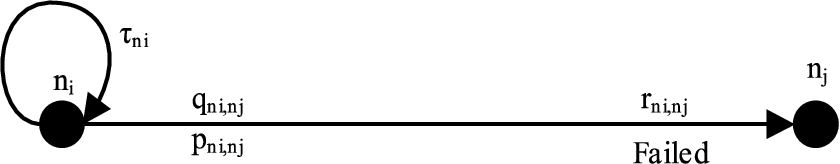
Assuming that the size of the reference packet is denoted as B and the probability of successful transmission of the link is
Equation (1) uses the link failure probability in measuring the quality of WMN links, which reflects the inherent uncertainty characteristic of wireless transmission in WMN.
2.2.2.Calculation of the remaining capacity of the path
Based on the above WMN transmission process, we can calculate the remaining capacity of the path. Assume that U denotes a given path, T denotes the remaining capacity of the routing protocol for that path [14], and C denotes the capacity occupied by the data stream currently being transmitted on that path. However, the difference between the two is the remaining capacity of that path R.
In a real network, it is also necessary to add a smoothing factor to integrate the channel interference effects around the path [3,8], to better match the actual network environment, which gives an approximate expression for the theoretical residual capacity
The capacity C occupied by the data stream currently being transmitted by the path is calculated as in Equation (4).
Combining the above calculations yields the final computational expression for the remaining capacity R of the path as in Equation (5).
2.3.Multipath network load balancing method design
According to the residual capacity of the path, a multi-path network load balancing method is designed. The multi-channel multi-interface approach is also known as the multi-channel multi-antenna approach. Multiple antennas are configured for each node in the network and then the channels are assigned to the antennas [4,10], which is used to improve the efficiency of data transmission. Using MCMR (Multi-channel multi-radio) method multiple interfaces are configured for the nodes in the network and channels are assigned to these interfaces so that inter-channel conflicts can be effectively avoided. This paper will combine the above indicators to improve the design of the multi-path load balancing method.
2.3.1.MCMR network topology design
Assuming that n denotes the nodes in the network, l denotes the link,
Fig. 2.
MCMR network topology schematic.
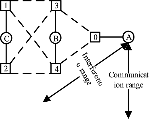
In Fig. 2, circles represent nodes in the network, squares represent interfaces configured on the nodes and dashed lines between interfaces represent assigned channels. Interface 0 is configured on the node A, interfaces 1, 2 on the node B, and interfaces 3 and 4 on the node C. The inter-interface relationships can be represented by an undirected graph, calculated as in Equation (6).
2.3.2.Design of routing criteria for load balancing in multipath network
In the AOMDV protocol, “hop count” is used as the routing criterion, which is easy to cause congestion in intermediate nodes and does not reflect the current load of the path explicitly. The study takes “interference” and “residual capacity” into consideration in the design of the routing criterion. First, the multipath interference model is established, and then the remaining capacity is taken as the current path load estimation. Finally, the interference-sensitive perceptive routing criterion is established considering the impact of interference on the path load to provide the basis for multi-path load balancing.
For the results of the inter-interface links calculated in Equation (6) above, the obtained links are numbered using L,
Total link interference
The interference present in a link is equal to the sum of the interference received by other links using the same channel. According to Equation (7), the interference received by the link
Sum of path disturbances
There are multiple links on a path, and the sum of the interference each link receives from the other links is used as an indicator of the interference on a path.
Remaining capacity
The load on the link can be measured by the remaining capacity on the interfaces at both ends of the link, the remaining capacity of the interface
The load on the path
Routing Criteria
In addition to the current load condition on the path, interference can also have an impact on the path load level. Two links will compete in the same channel and communication range. This will cause inter-link interference, which affects the quality of the wireless link, causing packets in the interface queue to wait and causing an increase in node load. Therefore, the interference factor of the path should also be considered as part of the impact path load indicator
2.4.Route discovery and path count control
Through the multi-path network load balancing method designed above, further control the route discovery and the number of paths. The AOMDV protocol can discover multiple paths, but only one primary path is used. The AOMDV protocol is improved so that it can discover and select multiple paths based on the routing criterion
The new field L,
2.5.AOMDV protocol improvement based on probabilistic triage
The improved AOMDV protocol on the one hand enables data to be transmitted with minimum energy relaying as much as possible, and on the other hand makes data change its original routing path with a certain probability, which avoids partial node overloading instead of balancing the nodes after the phenomenon of node overloading occurs. The improved AOMDV protocol is divided into two parts: routing path establishment and probabilistic equalization.
2.5.1.Routing path establishment
After controlling route discovery and number of paths, we can establish a route path. In the network, relay nodes are selected from their characteristic distances according to the coordinates of neighbor nodes to achieve minimum capacity relay. At the same time, a candidate node with the most remaining energy [9,13] is selected from the neighbor nodes for this node. If the remaining energy of the candidate node is more than this node, it is considered that a routing path with a light load is found from the multipath.
Assuming that the distance between a node S and the sink node is denoted as D, when D satisfies the condition in Equation (13), node S takes the sink node as the next hop directly without passing the relay node. Otherwise, node S selects node H which is closest to node S among all nodes
The candidate relay node
2.5.2.Probabilistic equilibrium for multipath routing protocols
Through the established routing path, the probability of multi-path routing protocol is balanced. During data transmission, a node uses candidate nodes as trunks with a certain probability to transfer data from the heavily loaded routing path to the lightly loaded routing path, which is called path switching[7]. Path switchover down hop count for data is set in which the initial value is 1. When the value is 0, data path switchover is prohibited.
Assuming that the remaining energy of each node in the network at a given moment is
If the node
We require timely updates to candidate node
According to the above rules, multipath data transmission with improved AOMDV protocol can be implemented.
Analyzing the difference in energy consumed by each node in the network in transmitting unit data, it is known that the closer the aggregation node bears the heavier the load of the relay, the more energy consumed is increasing and the residual energy is decreasing. Assuming that the residual energy of each path in the network
If a node
As the size of each path varies, the degree of the load varies during data transmission and the residual energy of the nodes has variability. The above probabilistic shunting method allows each node to switch paths with a certain probability during each data transmission, forwarding the data to the node with more residual energy, namely the path with a lighter load, so that the energy consumption of each path is equalized and the premature death of some nodes due to heavy load is avoided.
3.Experimental methods
3.1.Experimental environment
To verify the routing protocol in this paper, simulation experiments are conducted in a MATLAB environment using NS2 network simulation software, and the effectiveness and performance of the proposed routing protocol in this paper are analyzed based on the simulation. A modified AOMDV protocol with distributed coordination mechanism is used in the simulation environment, and the transmission rate of the wireless link is 54 Mbps. 30 CBR and VBR service flows are randomly generated during the experiment, and three routing algorithms WCETT-LB, MMESH, and Cluste_MMESH are deployed in the simulation environment. In 1000 m × 1000 m network coverage, the number of nodes deployed in a general WMN is 50 ∼80. When the number of nodes exceeds 80, the scale of the network is larger and the requirements for the routing protocols deployed in the network are higher. The parameters in the simulation experiments are set as shown in Table 1.
Table 1
Simulated environmental parameters
| Parameters | Setpoint |
| Network coverage | 1000 × 1000 |
| Number of nodes/pc | 20, 40, 60, 80, 100 |
| Data transfer rate/Mbps | 54 |
| Number of channels/pc | 15 |
| Channel bandwidth/Mbps | 12 |
| Data transmission range/m | 300 |
| Interference range/m | 600 |
| Number of business flows | 30 |
| Type of business flow | UDP |
| Data transmission method | CBR, VBR |
| Experimental run time | 600 s |
In this paper, the experiments use a 15-node experimental network topology diagram, using five computers and a switch to virtualize the experimental network, mainly for data success delivery rate, redundancy, network survival time, and network node survival number, using multiple experimental sampling, which takes the average of the method to optimize the above parameter value settings. The experimental network topology diagram is shown in Fig. 3.
Fig. 3.
Schematic diagram of the experimental network topology.
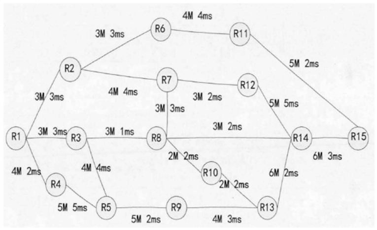
The number of each node in Fig. 3 is
In the simulation results, the following four metrics are used to evaluate the performance of the routing protocol in this paper. i) successful delivery rate is the probability that the source node can correctly receive a packet when it is sent by the aggregation node, which reflects the reliability of the network, the higher the value is, the higher the network reliability is, and vice versa ii) standard residual degree, the total number of times the aggregation node needs to send a packet when it correctly receives it, the lower the redundancy is, the higher the energy efficiency of the network is, and vice versa. iii) network survival time is how much time the network has remaining energy to send packets from the source node to the destination node, the longer the lifetime is, the higher the success rate of the transmission node is, and vice versa. iv) the number of nodes in the network is the number of nodes in the network that can continue to transmit data after some time, the more nodes survive, the more balanced and efficient the energy load of network nodes.
3.2.Performance analysis
3.2.1.Successful delivery rate
Successful delivery rate is defined in Equation (15), where M denotes the number of hops elapsed during data transmission. Furthermore, J denotes the packet length,
The simulation system sends a certain number of original packets from the source node, and then counts the number of packets successfully received by the aggregation node. The successful delivery rate is obtained by comparing the number of successfully received packets with the total number of packets sent by source node
Fig. 4.
Comparison of successful delivery rates before and after improvements to the AOMDV protocol.
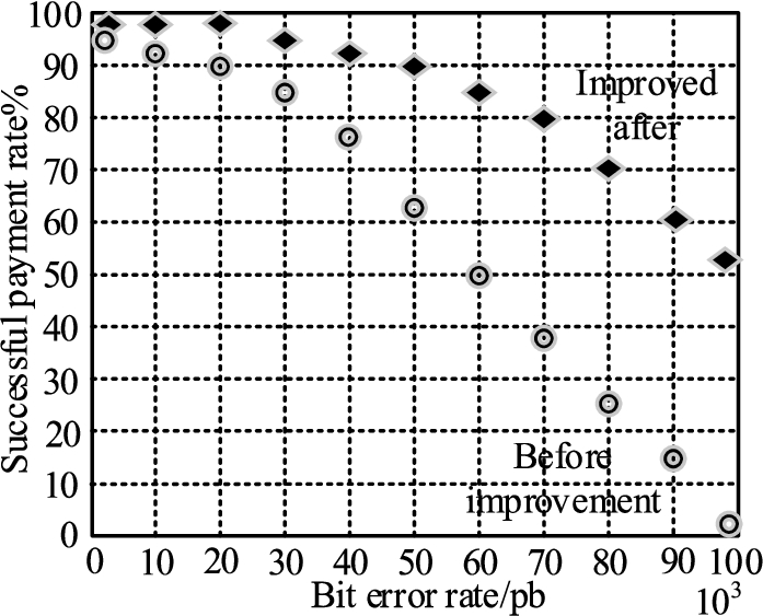
From Fig. 4, it can be seen that the successful delivery rate is not much different before and after the improvement of the AOMDV protocol in the case of very small BER, which is because when the BER is very small the data transmission process is almost error-free, so the successful delivery rate is very high. As the BER keeps increasing, the successful delivery rate of the pair before the improvement of the AOMDV protocol decreases significantly and drops to 0 when the BER reaches 100. The successful delivery rate of AOMDV protocol after improvement is always higher than 50%, which is because the improved AOMDV protocol adopts a multipath probability sending and probability balancing mechanism, which can quickly recover the routing path and improve the successful delivery rate of packet transmission when there is a problem in multipath routing.
3.2.2.Redundancy
Redundancy is calculated using Equation (16) where
Fig. 5.
Comparison of standardized redundancy before and after AOMDV protocol improvement.
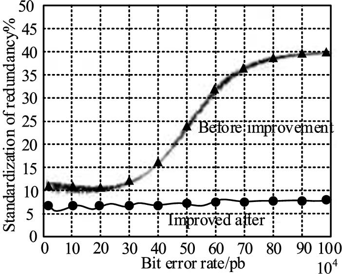
The redundancy reflects the energy consumption of the network because the total packets sent by the network are proportional to energy consumption. When redundancy is lower, it shows the higher energy effectiveness of the network, seeing that the redundancy is related to the successful delivery rate, which explains the reason why the redundancy increases with the BER in Fig. 5. As can be seen from Fig. 5, with the increase of bit error rate, the redundancy of the AOMDV routing protocol before improvement is also increasing. With the improved AOMDV routing protocol, although the bit error rate is increasing, the redundancy can maintain a more stable state, and the redundancy increases slowly. The establishment and probability equalization of multiple routing paths increase the success delivery rate, thereby reducing the redundancy.
3.2.3.Network survival time
Network survival time is defined as how much time the network has remaining energy to send packets from source node to destination node. If the node energy is limited, each source node tries to deliver data packets to the sink node. The simulation program is used until the node failure message cannot be delivered, and the effective time is recorded. The comparison of the network survival time under the AOMDV routing protocol before and after using the improvement is shown in Fig. 6.
Fig. 6.
Comparison of network survival time before and after AOMDV routing protocol improvement.
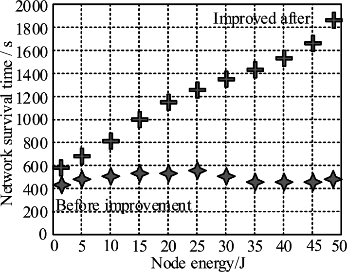
From Fig. 6, it can be seen that the network survival time is closely related to the energy of the nodes, and the higher the energy of the nodes, the longer the effective life cycle of the network. The network life cycle of the improved AOMDV routing protocol is better than that of the original AOMDV routing protocol. This is because the improved AOMDV routing protocol establishes multi-path routing and carries out probability balance, so that the data is sent to the link with more residual energy and less data, and the energy of the whole network can be balanced. As a result, the life cycle of the network is greatly improved.
3.2.4.Number of nodes surviving in the network
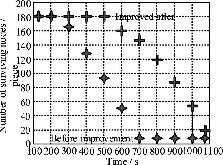
The number of node stocks in the network is defined as how many nodes in the network are continuing to transmit data after a given period, which varies with time. The number of node stocks in the network for the pre-improved and improved AOMDV routing protocols is shown in Fig. 7.
Observing Fig. 7, it can be found that the pre-improved AOMDV routing protocol has some nodes in the network beginning to die at 300 seconds (s) and all nodes in the network die when reaching 700 s. However, the improved AOMDV routing protocol delayed the node death by 200 s, because the improved AOMDV routing protocol adopted the method of probability shunt to make the energy load of network nodes more balanced and more effective. When the protocol reaches 1000 s, there are still surviving nodes in the improved AOMDV routing protocol, while all the nodes of the pre-improved AOMDV routing protocol have already died by this time. It can also be seen from Fig. 7 that when nodes start to die in the AOMDV routing protocol network before and after the improvement, the death rate of the remaining surviving nodes is gradually accelerated, which is because the remaining surviving nodes take on more data forwarding tasks and accelerate the death rate of the nodes.
Fig. 7.
Comparison of the number of nodes surviving in the network.
In this paper, several metrics are tested on the routing protocol using MATLAB and NS2 simulation tools, namely (i) successful delivery rate, (ii) redundancy, (iii) network survival time, and (iv) number of surviving nodes in the network. The test results validate the superiority of the multipath load balancing routing protocol based on the probabilistic diversion proposed in this paper.
4.Conclusion
As one of the key technologies in WMN, a routing protocol is directly related to the operation efficiency of the entire network. This paper focuses on how to establish efficient and reliable routing for wireless sensor networks. First, the advantages of multipath routing protocols are explored in WMN, then the improvement of AOMDV routing protocols is discussed on multipath routing performance. This is followed by looking at the advantages of probabilistic diversion in establishing energy-efficient multipath. Finally, this paper combines multipath routing establishment and probabilistic balancing methods to design and implement a load-balancing routing protocol for multipath networks based on probabilistic triage, which improves the energy efficiency and reliability of WMN.
An improved load-balancing routing protocol for a multipath network is proposed to solve the problem of unbalanced protocol communication in WMN in our research work. Simulation results show that the successful delivery rate of the improved AOMDV protocol is always higher than 50%, and the redundancy is lower than 10%. The node starts to die in 200 s. It is proved that the proposed protocol can effectively balance the node load and prolong the network lifetime, and the network congestion caused by node overload can be avoided in advance by a probabilistic shunt strategy, which reduces redundancy. In the aspect of multi-path generation, in addition to factors such as energy and number of surviving nodes, other influencing factors should also be considered. In future research, changes in packet transmission delay should be considered when the traffic in the network increases instantaneously to improve the rationality of the algorithm.
Acknowledgements
This paper was supported by the Provincial High-level Specialty Group Construction Project of Guangdong Higher Vocational Colleges (No. GSPZYQ20200069).
Conflict of interest
None to report.
References
[1] | A.M. Alatwi and A.N.Z. Rashed, Abd El Aziz I A. High speed modulated wavelength division optical fiber transmission systems performance signature, Telkomnika (Telecommunication Computing Electronics and Control) 19: (2) ((2021) ), 380–389. doi:10.12928/telkomnika.v19i2.16871. |
[2] | S.A. Alghamdi, Cuckoo energy-efficient load-balancing on-demand multipath routing protocol, Arabian Journal for Science and Engineering 47: (2) ((2022) ), 1321–1335. doi:10.1007/s13369-021-05841-y. |
[3] | K. Bechta, J.M. Kelner, C. Ziółkowski and L. Nowosielski, Inter-beam co-channel downlink and uplink interference for 5G new radio in mm-wave bands, Sensors 21: (3) ((2021) ), 793. doi:10.3390/s21030793. |
[4] | M. Benzaghta and K.M. Rabie, Massive MIMO systems for 5G: A systematic mapping study on antenna design challenges and channel estimation open issues, IET Communications 5: (13) ((2021) ), 1677–1690. doi:10.1049/cmu2.12180. |
[5] | G. Cerar, H. Yetgin, M. Mohorčič and C. Fortuna, Machine learning for wireless link quality estimation: A survey, IEEE Communications Surveys & Tutorials 23: (2) ((2021) ), 696–728. doi:10.1109/COMST.2021.3053615. |
[6] | M. Elhoseny and K. Shankar, Reliable data transmission model for mobile ad hoc network using signcryption technique, IEEE Transactions on Reliability 69: (3) ((2020) ), 1077–1086. doi:10.1109/TR.2019.2915800. |
[7] | W. Fu, S. Liu and S. Gautam, Optimization of big data scheduling in social networks, Entropy 21: ((2019) ), 902. doi:10.3390/e21090902. |
[8] | Z. Guo and S. Liu, Wireless image transmission interference signal recognition system based on deep learning, Wireless Communications and Mobile Computing 2021: ((2021) ), 8024953. |
[9] | L. Hu, H. Yan, L. Li, Z. Pan, X. Liu and Z. Zhang, MHAT: An efficient model-heterogenous aggregation training scheme for federated learning, Information Sciences 560: ((2021) ), 493–503. doi:10.1016/j.ins.2021.01.046. |
[10] | B. Jia, S. Liu, Y. Guan, W. Li and W. Ren, The fusion model of multi-domain context information for the Internet of things, Wireless Communications and Mobile Computing 2017: ((2017) ), 6274824. |
[11] | M. Jude, V.C. Diniesh, M. Shivaranjani, S. Madhumitha, V.K. Balaji and M. Myvizhi, Improving fairness and convergence efficiency of TCP traffic in multi-hop wireless network, Wireless Personal Communications 121: (1) ((2021) ), 459–485. doi:10.1007/s11277-021-08645-3. |
[12] | Q.V. Khanh, An energy-efficient routing protocol for MANET in Internet of Things Environment, iJOE 17: (07) ((2021) ), 89. |
[13] | A. Naeem, A.R. Javed, M. Rizwan, S. Abbas, J.C.W. Lin and T.R. Gadekallu, DARE-SEP: A hybrid approach of distance aware residual energy-efficient SEP for WSN, IEEE Transactions on Green Communications and Networking 5: (2) ((2021) ), 611–621. doi:10.1109/TGCN.2021.3067885. |
[14] | Y. Natarajan, K. Srihari, G. Dhiman, S. Chandragandhi, M. Gheisari, Y. Liu, C.C. Lee, K.K. Singh, K. Yadav and H.F. Alharbi, An IoT and machine learning-based routing protocol for reconfigurable engineering application, IET Communications 16: (5) ((2022) ), 464–475. doi:10.1049/cmu2.12266. |
[15] | T. Okumura, M. Murakami, Y. Uematsu, S. Okamoto and N. Yamanaka, Fault-tolerant multi-path routing method under high network failure environment, IEICE Technical Report; IEICE Tech. Rep 121: (76) ((2021) ), 33–39. |
[16] | M. Park and J. Paek, On-demand scheduling of command and responses for low-power multihop wireless network, Sensors 21: (3) ((2021) ), 738. doi:10.3390/s21030738. |
[17] | D. Pérez-Adán, Ó. Fresnedo, J.P. González-Coma and L. Castedo, Intelligent reflective surfaces for wireless network: An overview of applications, approached issues and open problems, Electronics 10: (19) ((2021) ), 2345. |
[18] | S.P. RM, S. Bhattacharya, P.K.R. Maddikunta et al., Load balancing of energy cloud using wind driven and firefly algorithms in Internet of everything, Journal of Parallel and Distributed Computing 142: ((2020) ), 16–26. doi:10.1016/j.jpdc.2020.02.010. |
[19] | C.C. Vignesh, C.B. Sivaparthipan, J.A. Daniel, G. Jeon and M.B. Anand, Adjacent node based energetic association factor routing protocol in wireless sensor network, Wireless Personal Communications 119: (4) ((2021) ), 3255–3270. doi:10.1007/s11277-021-08397-0. |
[20] | W. Wang, G. Srivastava, J.C.W. Lin et al., Data freshness optimization under CAA in the UAV-aided MECN: A potential game perspective, IEEE Transactions on Intelligent Transportation Systems 25: ((2020) ), 1–10. |
[21] | H. Yan, M. Chen, L. Hu and C. Jia, Secure video retrieval using image query on an untrusted cloud, Applied Soft Computing. 97: (A) ((2020) ), 106782. doi:10.1016/j.asoc.2020.106782. |
[22] | M.B. Yassien, S.A. Aljawarneh, M. Eyadat and E. Eaydat, Routing protocol for low power and lossy network-load balancing time-based, International Journal of Machine Learning and Cybernetics 12: (11) ((2021) ), 3101–3114. doi:10.1007/s13042-020-01261-w. |


