
Analysis on the low-frequency electromagnetic pulse coupling to horizontal electrically short lines
Abstract
In this study, we investigated the coupling features of the nuclear electromagnetic pulse (NEMP) on overhead cables in the middle-and-far regions, different from the transmission line model commonly used for field-line coupling in high-frequency cases, using a simpler lumped approximation to solve the electrically small size model in low-frequency cases. To verify its effectiveness, a simulation model with the same conditions was set up using the software of Computer Simulation Technology (CST), and cable coupling experiments were performed in a laboratory environment using a bounded-wave electromagnetic pulse simulator. The calculated results of the lumped approximation circuit were compared with the CST simulation and measured results, and the agreement was good. The results also shows that the load exhibits a differential response in the case of the low impedance and it is consistent with the excitation signal in the case of the high impedance. Finally, some more experiments were constructed to analyzed the effect of different cable parameters on the cable load response through experiments, and the experimental results are also in general agreement with the theoretical analysis, in which the induced signal of the low-impedance load is mainly determined by the magnetic field in the direction normal to the cable and the ground loop and the induced signal of the high-impedance load is mainly determined by the electric field in the direction of the height of the cable erection.
1.Introduction
Electromagnetic pulses (EMPs) are generated by the Compton effect when a nuclear explosion occurs. The spectrum of nuclear electromagnetic pulse (NEMP) is very wide, ranging from low to ultra-high frequency. During propagation, the signal attenuation varies at different frequencies; thus, the EMP waveform varies with distance. The high-frequency component, due to its short wavelength, large ground loss, and poor bypassing ability, cannot propagate over long distances. The low-frequency component propagates with little attenuation in the ground-ionosphere waveguide, and when the EMP propagates to the far regions, it decays into a simple very-low-frequency pulse waveform with its main energy distribution at 0–100 kHz [1]. The second type of pulse waveform (0.4 μs rising edge, 10 μs half pulse width) and the third type of pulse waveform (3 μs rising edge, 30 μs half pulse width) in GJB 3634-99 are commonly used to simulate the waveform of the medium and long-range NEMP [2]. Compared with high-altitude nuclear electromagnetic pulses (HEMPs), medium and long-range NEMPs exhibit increased high-frequency component attenuation, a rapid decrease in electric field amplitude, and the destructive effect on electronic and electrical equipment is no longer significant because of the increase in propagation distance; therefore, detection in the medium and long-range region has more scientific value and military significance. However, long-range detection of nuclear explosions requires the use of different detection methods, as well as the study of the corresponding signal propagation and coupling laws. This study focuses on the coupling effect of the medium and long-range NEMP on overhead lines.
The coupling problem of EMPs on overhead lines is mainly divided into two, namely, low-frequency problems for electrically short lines and high-frequency problems for electrically long lines, which can usually be solved by different methods [3], which can be divided into three main categories in order of complexity, such as quasi-static field methods [4], classical transmission line theory [5–7], and full-wave simulation analysis. Transmission line models are mainly analyzed for long-line models in high-frequency cases, where the influence of wave propagation effects on the line must be considered, whereas short-line models in low-frequency cases can be viewed as lumped approximation circuits of electrically small size. Numerous theoretical analyses have been performed by various scholars to determine the effectiveness of field-line coupling of transmission line models. Andreotti [8] found that, under certain conditions, the transmission line approximation method can obtain the same results as the more rigorous full-wave analysis methods, and Nucci [9] conducted a comparative study of three transmission line models, and the results showed that these three transmission line models can produce the same response results. Based on the classical transmission line theory, Tesche [10] derived the frequency domain Baum–Liu–Tesche (BLT) equation to solve the transmission line terminal response and the time-domain BLT equation to solve the transmission line terminal nonlinear load [11]. Paul [12] proposed the SPICE model to solve the transmission line response. In addition, Tkatchenko [13,14] proposed an iterative algorithm to solve a set of coupled equations based on perturbation theory, which generalizes the classical transmission line equation to a generalized transmission line equation that includes high-frequency radiation effects. Guo [15] used the asymptotic method and extended it to the lossy ground case to improve computational efficiency in computing long lines. Unlike the long-line coupling problem in the high-frequency case, this study focused on the short-line coupling problem in the low-frequency case, particularly the coupling problem of the NEMP on the electrically short line in the middle-and-far regions. A simple approximate method is used to equate the distributed excitation source of the incident field effect to the lumped excitation source, and a lumped approximation circuit is constructed to Pspice to solve the response on the load for the overhead line that meets the electrically small size on the perfectly conducting ground. In addition, many scholars have conducted a series of experiments on cable coupling in the presence of high-frequency EMP to verify the accuracy of the transmission line model in solving the long-line problem [16–18]. The field-line coupling experiments of meeting the electrically small size lack corresponding research for the low-frequency EMP. According to GJB 3634-99, the second category of NEMP waveform, this study first analyzes the coupling effect of NEMP in the middle-and-far regions on the overhead cable, and then the corresponding experiments are performed, and the experimental results agree well with the calculation and simulation results of this study, proving the correctness of the theoretical analysis which implies that the induced signals at the load are associated with different electromagnetic field components for different load states.
2.Electrically small size model in low-frequency case
The electromagnetic field coupling to the cable is divided into different cases according to the cable coupling length l and signal wavelength 𝜆. When the line length l < 10𝜆 (for the EMP this means that the line length l < ctr∕10, where tr is the rising edge time of the EMP), the field-line coupling event can be regarded as a low-frequency case. In this condition, the distribution parameters on the cable can be considered uniform, and using the lumped approximation circuit can fully express its characteristics. When the line length l > 10𝜆, (for the EMP this means that the line length l > ctr∕10), the distribution parameters on the cable for the high-frequency case are not uniform, thus the transmission line equation must be used to solve [12].
Fig. 1.
Electromagnetic field coupling to overhead lines under incident wave excitation.
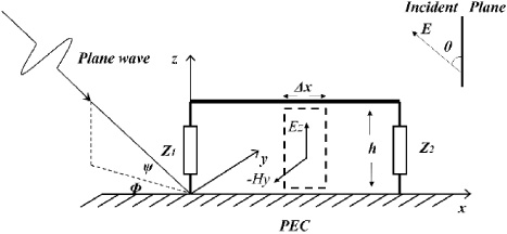
According to the Taylor model, when a uniform plane wave is incident, the frequency domain expression for the coupling of an EMP on a perfectly conducting ground to a unit length of the cable is as follows:
(1)
(2)
(3)
(4)
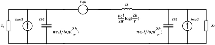
A lumped 𝛱-type circuit can be used for equivalence in the low-frequency case for a single cable on the ground. The field-line coupling model can be analyzed for the low-frequency case with an electrically small size by including the irradiation effect of the incident field in the lumped circuit. The incident field applies an equivalent voltage and current source at each point on the line because the impact of the propagation effect on the line is ignored, and the equivalent source is multiplied by the total line length to obtain the total lumped source. A cable of length l that meets the low-frequency case is equated using a lumped approximation circuit (Fig. 2), where the line length is l. The total capacitance in this total set parameter circuit is Cl, the total inductance is Ll, and the total lumped voltage and current sources in the frequency domain are as follows:
(5)
(6)
Converting a frequency-domain lumped source into a time-domain lumped source by time-frequency transformation:
(7)
(8)
According to Fig. 2, the 𝛱-type lumped approximation circuit model is built in Pspice, and the time-domain lumped sources Vn(t) and In(t) containing the incident field effects are used as program inputs, and the time-domain waveform on the load is obtained after running the program.
Fig. 2.
The 𝛱 type lumped approximation circuit.
3.Calculation and simulation analysis
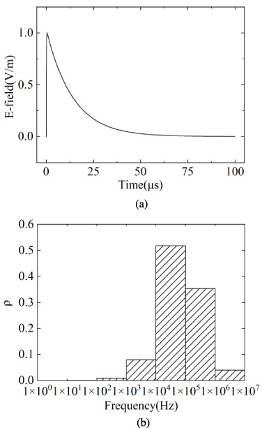
In this study, the second type of NEMP waveform in GJB 3634-99 is studied to simulate the NEMP in the middle-and-far regions. This time-domain waveform and the energy density distribution are shown in Fig. 3. The time-domain expression of an EMP with 0.4 μs rising edge and 10 μs half pulse width is expressed as follows:
(9)
Fig. 3.
0.4/10 μs NEMP. (a) Time-domain waveform. (b) Energy density distribution.
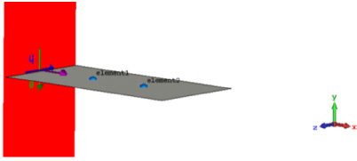
Generally, full-wave simulation can produce more accurate results. To validate the model, the time-domain finite integration method in the electromagnetic simulation software, CST is used, and the time-domain waveforms and transfer functions obtained from the solution are compared with the solution results of the lumped approximation circuit model constructed in Pspice. Next, we will discuss the two cases of electrically small size overhead lines for low and high impedance loads. The overhead cable model of CST is built as shown in Fig. 4. The theoretical calculation and CST simulation parameters are listed in the table below:
Table 1
The parameters of examples
| Cases | Incident wave (0.4/10 μs)𝜃 = 180°, 𝜓 = 0°, 𝜙 = 0° | L (H) | C (F) | ||
| Length (m) | Height (m) | Load (𝛺) | |||
| Low impedance | 1.3 | 0.04 | 2 | 1.5e-6 | 1.25e-11 |
| High impedance | 1.3 | 0.04 | 106 | ||
Fig. 4.
The overhead cable modeled in CST studio.
3.1.Low impedance at terminal loads
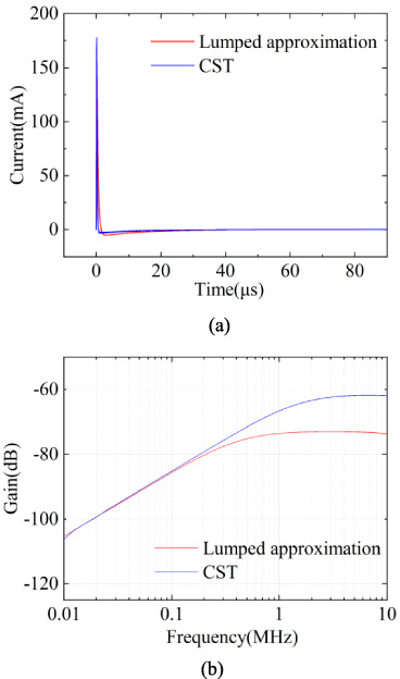
For low-impedance overhead lines (approximate short circuit at both ends), which mainly exhibit a current-type response, the terminal current response is solved using the lumped approximation circuit and the time-domain finite integration technique in CST, respectively. In Fig. 5, it is clear that the solution results of the two methods are in good agreements. Meanwhile, it can be found that in the main frequency range of the excitation signal, when the overhead line is terminated with the low-impedance load at both ends, the load response is mainly exhibited as the differential form of the excitation signal.
Fig. 5.
Time and frequency domain responses of different solutions under the low impedance condition. (a) Time domain responses. (b) Frequency domain responses.
Obviously, the line length and height of overhead lines are the main factors affecting its load response. Therefore, we construct the corresponding models in the electromagnetic simulation software CST to analyze the influence of these two factors on the load response in the case of low impedance loads, respectively. The relevant model parameters are shown in Table 2 and Table 3.
Table 2
Cases of different lengths at low impedance
| Cases | Incident wave (0.4/10 μs)𝜃 = 180°, 𝜓 = 0°, 𝜙 = 0° | ||
| Length (m) | Height (m) | Load (𝛺) | |
| Case1 | 1.3 | 0.04 | 2 |
| Case2 | 0.9 | 0.04 | 2 |
| Case3 | 0.5 | 0.04 | 2 |
Table 3
Cases of different heights at low impedance
| Cases | Incident wave (0.4/10 μs)𝜃 = 180°, 𝜓 = 0°, 𝜙 = 0° | ||
| Length (m) | Height (m) | Load (𝛺) | |
| Case1 | 1.3 | 0.04 | 2 |
| Case2 | 1.3 | 0.08 | 2 |
| Case3 | 1.3 | 0.12 | 2 |
Fig. 6.
Effects of cable lengths on the load response under the low impedance condition. (a) Time domain response. (b) Frequency domain response.
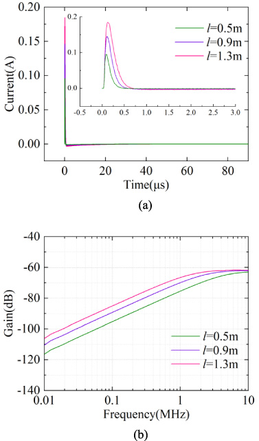
Viewing Fig. 6(a), as the cable length increases, the amplitude of the induced current at the terminal load increases, and the trend of the time domain waveform remains basically unchanged. In Fig. 6(b), it can be seen that as the cable length increases, the upper turning frequency of its frequency response decreases, implying that the available frequency range decreases.
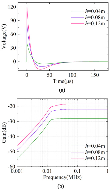
Fig. 7.
Effects of cable heights on the load response under the low impedance condition. (a) Time domain response. (b) Frequency domain response.
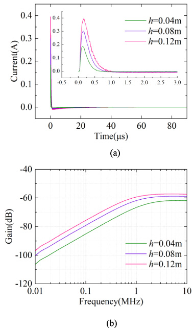
Similarly, according to Fig. 7, It shows that as the height of the cable increases, the amplitude of the induced current at the terminal load increases, and the trend of the time domain waveform remains basically the same, however, the upper turning frequency of the frequency response decreases.
So we can infer that under the low impedance condition, the cable forms a loop with the ground, and the sensitivity of its load response is mainly related to the magnetic field Hy (Fig. 1) in the direction normal to the plane of the loop. Increasing the length and height of the cable can make its sensitivity higher, but it will lower its upper cutoff frequency.
3.2.High impedance at terminal loads
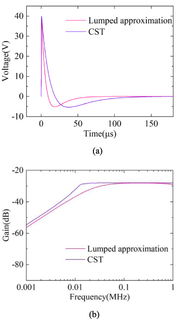
For high impedance overhead lines (approximate open circuit at both ends), which mainly exhibits a voltage-type response, the terminal voltage response is solved using the lumped approximation circuit and the time-domain finite integration technique in CST, respectively (Fig. 8). The solution results of the two methods also maintain a good agreement. Also, we can find that the load response in the case of the high impedance essentially remains the same as the excitation signal in the main frequency range.
Fig. 8.
Time and frequency domain responses of different solutions under the high impedance condition. (a) Time domain response. (b) Frequency domain response.
Furthermore, the corresponding models were constructed in the electromagnetic simulation software CST to analyze the effects of these two factors on the overhead line load response under high impedance loads, and the relevant model parameters are shown in Tables 4 and 5.
Table 4
Cases of different lengths at high impedance
| Cases | Incident wave (0.4/10 μs)𝜃 = 180°, 𝜓 = 0°, 𝜙 = 0° | ||
| Length (m) | Height (m) | Load (𝛺) | |
| Case1 | 1.3 | 0.04 | 106 |
| Case2 | 0.9 | 0.04 | 106 |
| Case3 | 0.5 | 0.04 | 106 |
Table 5
Cases of different heights at high impedance
| Cases | Incident wave (0.4/10 μs)𝜃 = 180°, 𝜓 = 0°, 𝜙 = 0° | ||
| Length (m) | Height (m) | Load (𝛺) | |
| Case1 | 1.3 | 0.04 | 106 |
| Case2 | 1.3 | 0.08 | 106 |
| Case3 | 1.3 | 0.12 | 106 |
Figure 9 shows that as the line length increases, the amplitude of the induced voltage at the terminal load of the overhead cable remains constant. The change in line length mainly affects the response of the lower turning frequency, and the response of other high-frequency parts is basically unaffected. At the same time, it shows that the line height mainly affects the magnitude of the induced voltage at the terminal load. With the increase in line height, the induced voltage at the terminal load also increases, which basically makes no impact on the frequency response of each frequency band (Fig. 10).
Therefore, we can infer that under high impedance conditions, the cable does not form a loop with the earth, and the sensitivity of its load response is mainly related to the electric field Ez (Fig. 1) in the direction of the cable erection height. Increasing the length of the cable only changes the inductance of the cable, affecting the lower cut-off frequency, while increasing the height of the cable only makes its sensitivity higher and does not affect the lower cut-off frequency.
Fig. 9.
Effects of cable lengths on the load response under the high impedance condition. (a) Time domain response. (b) Frequency domain response.
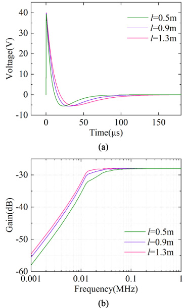
Fig. 10.
Effects of cable lengths on the load response under the high impedance condition. (a) Time domain response. (b) Frequency domain response.
Subsequently, to further verify the correctness of the theoretical analysis, some experiments will be conducted in a laboratory.
4.Field-line coupling experiments with bounded-wave electromagnetic pulse simulator
Experiments are performed in this section to further verify the accuracy of the theoretical analysis. The experiment is performed using a vertically polarized bounded-wave EMP simulator with a working effect interval of 1.5 × 1.5 × 1.2 m and a NEMP simulation signal generator. The device can simulate the second type of nuclear explosion EMP environment in GJB 3634-99 in the bounded-wave working effect space with a field strength range of 100–8000 V/m, and the work is stable. A 1.3-m long thin wire with a radius of 0.25 mm, which is an insulation layer of metal copper wire, was erected on a plastic bracket, the thin wire ends were connected to resistors connected to the lower pole plate to the ground. For low impedance loads, Rogowski coils were used to measure the induced current, and for high impedance loads, the voltage at the terminal load was measured directly. The schematic of the entire experimental layout is shown in Fig. 11, and the actual experimental system build site diagram is shown in Fig. 12. The monopole antenna with the frequency range of 10 kHz–30 MHz is used to measure the electric field. For low impedance cases, the CYBERTEK’s HCP8030 Rogowski coil with the frequency range of DC–50 MHz is looped over the wire near the terminating resistor and connected to the Tektronix DPO 3032 digital oscilloscope for displaying and saving measured induced current data. The range of this current probe is 0–5 A and 0–30 A, corresponding to the current transmission ratio of 1 and 0.1 V/A, and the small range is selected. For high impedance cases, the matching voltage probe is connected to a terminating resistor and linked to a Tektronix DPO 3032 digital oscilloscope for displaying and saving measured induced voltage data.
Fig. 11.
Schematic of the experimental layout.
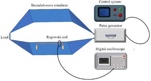
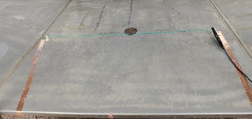
Fig. 12.
Site diagram of actual experimental system construction.
4.1.Comparison of the experimental and calculated results
When performing EMP cable coupling experiments in the built experimental system environment, the actual electric field waveform measured by placing the monopole antenna at the center of the polar plate under the bounded wave, the peak incident electric field 1050 V/m, fitting the measured electric field waveform with a double exponential function, and the fitting parameters are shown in Eq. (9). The measured and fitted normalized electric field waveforms are shown in Fig. 13.
Firstly, we discuss the case under low impedance loads. The induced current waveform on the measured load of the Rogowski coil is shown in Fig. 14. The thin wire in the experimental environment is erected on a perfectly conducting ground because the lower pole plate of the bounded-wave generator is a metal plate. The solution is performed using the lumped approximation circuit, and the expression of the fitted electric field E0(t) is substituted into the time-domain lumped voltage source Vn(t) and the time-domain lumped current source In(t) as the program input, comparing the calculated response current on the load with the response current on the load measured by the Rogowski coil (Fig. 15). CST is used for the solution, and the measured electric field is used as the excitation, comparing the response current on the load obtained from the CST simulation with the response current on the actual load measured using the Rogowski coil (Fig. 16).
Theoretical analysis shows that the signal on the load behaves in a differential form in the main frequency range of the excitation signal, and the measured signal on the load shown in Fig. 14 is digitally integrated. First, the measured signal is noise reduced, and the denoised signal still has zero drift because of the combination of an oscilloscope and experimental environment. According to the analysis, the error signal causing zero drift is mainly in the frequency range below 4 kHz. The measured signal after noise reduction is de-zero-drifted by filtering out the zero-drift error signal in this frequency range, Finally, the measured signal is digitally integrated after noise reduction and zero drift, and the digitally integrated signal is compared with the measured electric field signal (Fig. 17). The two are in good agreement, confirming that the response on the load is a differential form of the excitation signal, and the cause of partial errors is that new errors are indirectly introduced when the measured signal is processed by noise reduction and zero drift removal.
Fig. 13.
Measured electric field and fitted electric field normalized waveform.
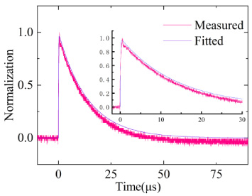
Fig. 14.
Measured current response on a high impedance load.
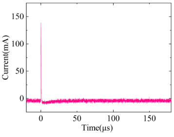
Fig. 15.
Comparison of lumped approximation calculation and measured results on a low impedance load.
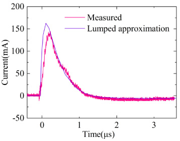
Fig. 16.
Comparison of CST calculations and measured results on a low impedance load.
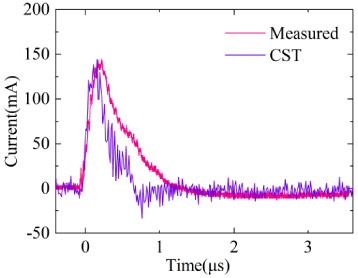
Fig. 17.
Comparison of digital integrated signals.
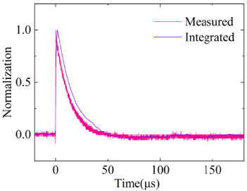
Fig. 18.
Measured voltage response on a high impedance load.
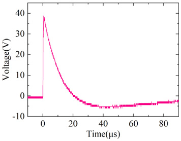
Fig. 19.
Comparison of lumped approximation calculation and measured results on a high impedance load.
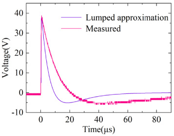
Fig. 20.
Comparison of CST calculations and measured results on a high impedance load.
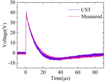
Next, we discuss the case under high impedance loads. The induced voltage waveform on the measured load is shown in Fig. 18. By using the lumped approximation circuit, comparing the calculated response voltage on the load with the measured response voltage directly (Fig. 19). CST is used for the solution, and the measured electric field is used as the excitation, comparing the response voltage on the load obtained from the CST simulation with the measured response voltage directly (Fig. 20). It can be noted that under the high impedance load, the full-wave simulation results are in good agreement with the measured results, while the lumped-parameter approximation circuit solution results have a little difference with the measured results, which may be the reason that the lumped approximation circuit only considers the capacitance of the horizontal cable to the ground and ignores the capacitance of the vertical line segments of the load end to the ground.
4.2.Effects of different factors on the load response
From the previous simulation analysis, we already know that the line length and line height are significant factors affecting the load response of overhead cables. Here we also divided into two cases of low impedance loads and high impedance loads for discussion, and analyzed the effect of different cable parameters on the cable load response through experiments respectively.
For the case of low impedance loads, we conduct field-line coupling experiments in the bounded-wave simulator, varying the length and height of the overhead cable to observe the change in its load responses. The relevant experimental parameters are consistent as in Table 2 and Table 3.
Fig. 21.
Different current responses measured at low impedance conditions. (a) Changes of the line length. (b) Changes of the line height.
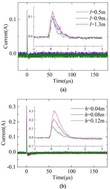
The experimental results in Fig. 21 show that as the cable length and height increase, the area of the loop composed of the cable and the ground increases, and the magnetic flux in the direction normal to the plane of the loop increases, resulting in an increase in the magnitude of the induced current at the load end.
For the case of high impedance loads, we also conduct field-line coupling experiments in the bounded-wave simulator, varying the length and height of the overhead cable to observe the change in its load responses. The relevant experimental parameters are consistent as in Table 4 and Table 5.
Fig. 22.
Different voltage responses measured at high impedance conditions. (a) Changes of the line length. (b) Changes of the line height.
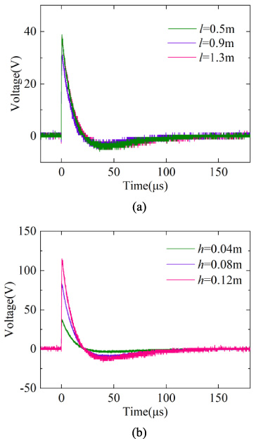
The experimental results in Fig. 22 show that the increase in cable length basically does not affect the magnitude and waveform trend of the induced voltage at the load end, while the increase in cable height leads to an increase in the magnitude of the induced voltage at the load end. This is attributed to the inductance change caused by the variation of cable length under high impedance load (approximately open circuit), which slightly affects the waveform of the induced voltage, but not the magnitude of the induced voltage. However, due to the presence of the overhead line capacitance to the ground, the voltage between the cable and the ground increases as the height of the cable grows.
All the above experimental results are consistent with the previous theoretical analysis. However, comparing the simulated and measured results under high impedance conditions, it can be found that there is a slight difference in the amplitude of the three measured results by changing the length of the cable, which is due to the fact that it cannot be guaranteed that the NEMP simulation signal generator will be charged with exactly the same voltage each time.
In fact, as one of the most closely connected and widely used application scenarios in human daily life, cables are capable of coupling to the low-frequency EMP. So we are able to choose a suitable overhead cable as a detection antenna to receive signal waveforms of interest to determine if particular types of things are happening.
Consequently, we can either choose cables that already exist in our lives or we can set up our own cables and detect the low frequency signals we are interested in by determining the loads at both ends. If a cable is the low impedance at both ends (approximately short circuit), then the load of the induced current sensitivity is greater, it can be obtained the current signal coupled in the cable by the Rogowski coil over the load side of the cable, and the coupled signal is the differential form of the original signal. If a cable is the high impedance at both ends (approximately open circuit), then the load of the induced voltage sensitivity is greater, it can be obtained the voltage signal coupled in the cable directly, and coupled signal remains consistent with the original signal.
5.Conclusion
In this paper, we carried out the coupling features of such low-frequency NEMP on overhead electrically short lines theoretically and experimentally. The results indicate that using the lumped approximation circuit can evaluate the response of the NEMP coupling to the cable in the middle-and-far regions when its racking conditions meet the electrically small size. Through theoretical and experimental analysis, it can be found that the terminal load presents a differential response of the excitation EMP when the horizontal overhead cable is terminated with the low impedance and it is consistent with the excitation EMP in the case of the high impedance. For the case of low impedance loads, the increase in the line length and height leads to a growth of induced current. But for the case of high impedance loads, the line height is the main factor affecting the magnitude of the induced voltage, which shows that the induced voltage at the terminal load is positively correlated with the line height. This provides a new idea that shows that the overhead cable meeting the conditions can be viewed as an electrically small size receiving antenna as a means of NEMP detection in the middle-and-far regions, and further investigates its application toward NEMP detection in the middle-and-far regions. Unlike the classical electrically small size antenna, the overhead cable has a larger equivalent area and thus has higher sensitivity in detecting low-frequency signals with weak field strength. It is also easy to set up and well camouflaged.
References
[1] | X. Liu, Z. Chen, H. Chen and Y. Liu, Introduction to the Detection of Nuclear Explosion Electromagnetic Pulses in far Areas, China Vision Press, Beijing, (1989) . |
[2] | General specification for nuclear electromagnetic pulse simulators for use of nuclear monitoring materiel, GJB3634-99, 1999. |
[3] | M. Brignone, F. Delfino, R. Procopio, M. Rossi, F. Rachidi and S.V. Tkachenko, An effective approach for high-frequency electromagnetic field-to-line coupling analysis based on regularization techniques, IEEE Trans. Electromagn. Compat. 54: (6) ((2012) ), 1289–1297. |
[4] | F.M. Tesche, M.V. Ianoz and T. Karlsson, EMC Analysis Methods and Computational Models, Wiley, New York, (1997) . |
[5] | C. Taylor, R. Satterwhite and C. Harrison, The response of a terminated two-wire transmission line excited by a nonuniform electromagnetic field, IEEE Trans. Antennas Propagat. 13: (6) ((1965) ), 987–989. |
[6] | F. Rachidi, Formulation of the field-to-transmission line coupling equations in terms of magnetic excitation field, IEEE Trans. Electromagn. Compat. 35: (3) ((1993) ), 404–407. |
[7] | A. Agrawal, H. Price and S. Gurbaxani, Transient response of multiconductor transmission lines excited by a nonuniform electromagnetic field, IEEE Trans. Electromagn. Compat. 22: (2) ((1980) ), 119–129. |
[8] | A. Andreotti, D. Assante, V.A. Rakov and L.L. Verolino, Electromagnetic coupling of lightning to power lines: Transmission-line approximation versus full-wave solution, IEEE Trans. Electromagn. Compat. 53: (2) ((2011) ), 421–428. |
[9] | C.A. Nucci and F. Rachidi, On the contribution of the electromagnetic field components in field-to-transmission line interaction, IEEE Trans. Electromagn. Compat. 37: (4) ((1995) ), 505–508. |
[10] | F.M. Tesche, Development and use of the BLT equation in the time domain as applied to a coaxial cable, IEEE Trans. Electromagn. Compat. 49: (1) ((2007) ), 3–11. |
[11] | F.M. Tesche, On the analysis of a transmission line with nonlinear terminations using the time-dependent BLT equation, IEEE Trans. Electromagn. Compat. 49: (2) ((2007) ), 427–433. |
[12] | C.R. Paul, Analysis of Multiconductor Transmission Lines, 2nd edn, Wiley, Hoboken, NJ, USA, (2008) . |
[13] | S. Tkatchenko, F. Rachidi and M. Ianoz, Electromagnetic field coupling to a line of finite length: Theory and fast iterative solutions in frequency and time domains, IEEE Trans. Electromagn. Compat. 37: (4) ((1995) ), 509–518. |
[14] | S. Tkatchenko, F. Rachidi and M. Ianoz, High-frequency electromagnetic field coupling to long terminated lines, IEEE Trans. Electromagn. Compat. 43: (2) ((2001) ), 117–129. |
[15] | J. Guo, F. Rachidi, S.V. Tkachenko and Y.-Z. Xie, Calculation of high-frequency electromagnetic field coupling to overhead transmission line above a lossy ground and terminated with a nonlinear load, IEEE Trans. Antennas Propagat. 67: (6) ((2019) ), 4119–4132. |
[16] | D. Hansen, H. Schaer, D. Koenigstein, H. Hoitink, H. Garbe and D.V. Giri, Response of an overhead wire near a NEMP simulator, IEEE Trans. Electromagn. Compat. 32: (1) ((1990) ), 18–27. |
[17] | Y. Xie, Z. Wang, Q. Wang, H. Xiang, X. Nie, H. Zhou , Experimental study on the response of aerial wires illuminated by simulated electromagnetic pulse, Proceedings of the CSEE 26: (24) ((2006) ), 200–204. |
[18] | H. Xie, Theoretical and experimental study of effective coupling length for transmission lines illuminated by HEMP, IEEE Trans. Electromagn. Compat. 57: (6) ((2015) ), 1529–1538. |
[19] | D. Poljak, F. Rachidi and S.V. Tkachenko, Generalized form of Telegrapher’s equations for the electromagnetic field coupling to finite-length lines above a lossy ground, IEEE Trans. Electromagn. Compat. 49: (3) ((2007) ), 689–697. |
[20] | G. Ni, J. Luo and C. Li, Comparison of solutions to the Taylor and Agrawal coupling models for the line-plane transmission-lines, Journal of National University of Defense Technology 29: (5) ((2007) ), 111–116. |


