Magnetic levitation stages for planar and linear scan application with nanometer resolution¹

1.Introduction

Magnetically levitated positioning stages (Mag-6D) have been developed since the 90s. Extremely accurate systems are used in the semiconductor industry for fine positioning of wafers [1,2]. The main advantages are the smooth and controllable accuracy and perfect cleanness during scan movements in relation to “standard” mechanically guided systems or air bearing systems. The stability and tracking performance depends only on the sensors, the drivers, and the control algorithms. On the other hand, the strong dependency of the positioning performance and the tracking accuracy is mainly defined by the use of high-quality sensor systems, low noise drivers and complex control algorithms. Inaccurate guiding has no influence - because there is no additional guiding.

Industrial applications require free access to the top plate of a movable platform. The top platform is the working area and sensor systems should not be placed there, and beams of interferometers should also not cross this area. There is also no way to detect the position of the platform from the upper side by using camera positioning equipment. The optical paths would be interrupted by the handling modules above. Usually, the platform carries the wafer chuck, the tool handling, and the clamping mechanism etc.

Searching for solutions in very price-sensitive applications with 6-DOF sensors leads to hard technical challenges. All of our measuring systems have to be installed on the bottom or on the side of the movable stage. Most of the high-resolution laser interferometers, confocal measuring systems etc. are so expensive that a system design with those types of measuring tools is possible but not relevant for certain industrial applications.

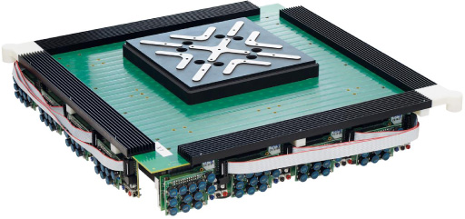
Fig. 1.

Planar magnetic levitation stage without cover, the coil drivers are on two sides.

2.Planar MAG_6D stage system structure

We describe a new magnetic levitation system (see figure 1) with nanometer resolution, where the maglev platform can be lifted and moved in space without any wired connection on it. We have shown in [4] that there is a minimum of 6 coils and three Halbach arrays, where the sensor system lays in the middle, below the stage and between the coils. That design works with high accuracy with the sensors in the middle of the stage. But for reasons of efficiency, it needs an expensive cooling system and it is not easy to scale. W. Kim and later X. Lu have shown that the driving coils can be placed in a printed circuit board (PCB) [2]. But in those applications, it was not possible to integrate low-price nanometer sensors.

Fig. 2.

Planar magnetic levitation stage. 1: Movable stage, 2: Halbach array (consist of 8 arrays), 3: 2-D optical grid, 4: Coil board (PCB with 144 coils), 5: Granite baseplate (nonmagnetic), 6: Sensor module with 7 sensor heads, 7: Current drivers (48 full bridges), 8: Cable setup and sensor connector modules, 9: Heat pipe for very low thermal hot spots.

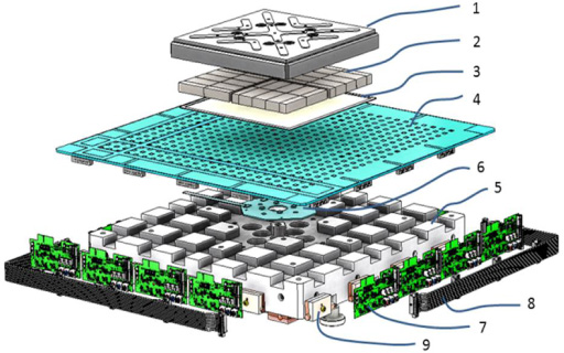
Our new planar maglev system (figure 2) combines a fully passive stage with 8 Halbach arrays and an optical sensor grid. The optical incremental sensor grid is placed onto the movable stage between the magnetic arrays and the coil board, which is placed on a granite baseplate. 7 optical incremental sensor heads, and additional four time 4 analog hall sensors are fixed on the light-weight granite base.

Most of industrial applications require free access to the movable top plate, which requires that all sensors should be placed below the platform. The main challenge for pushing the technology to the “industrial nanometer level” is to get it to work for low-price distance sensors with nanometer resolution and a motion range of millimeters.

Fig. 3.

Planar magnetic levitation stage with a set of 4 Halbach arrays, each consisting of two arrays because of better technological handling (top view).

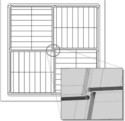
Figure 3 shows the arrangement of the 8 Halbach arrays in 4 groups. It is useful to align the X and Y direction of the Halbach arrays. The measured magnetic flux is shown in figure 4. This alignment with a small gap to the rectangular direction makes the magnetic field distribution continuous from one end to the other end of the stage. The 3-phase coil design is in phase with the magnetic field distribution.

Fig. 4.

Resulting measurement of the positive Z component of the magnetic flux density of the 4 Halbach arrays, the flux density Bz on this side of the Halbach is much higher than in the opposite direction, the stray field on top of the stage is low (bottom view onto the stage).

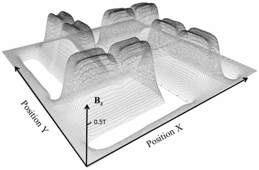
Fig. 5.

3-phase coil structure for 2 layers of the PCB, 12 or 24 layers are used. The 3 phases are shown by yellow lines for coils corresponding to the driving forces in the Y and Z direction.

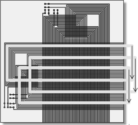
The coil design of one layer of the PCB is shown in Fig. 5. Both copper layers are used for the X and Y direction of the 3-phase driving coils. Figure 5 shows no gaps between the 3 phases of the coils. This coil structure provides high energy efficiency for force generation but there is no space for the sensors – viewed from the bottom through the PCB.

Fig. 6.

Coil structure of the 3 phases for 2 layers with gaps between the phases, rectangular, and round holes are places at some gaps. The yellow lines highlight the coil structure corresponding to the driving forces in the Y and Z direction.

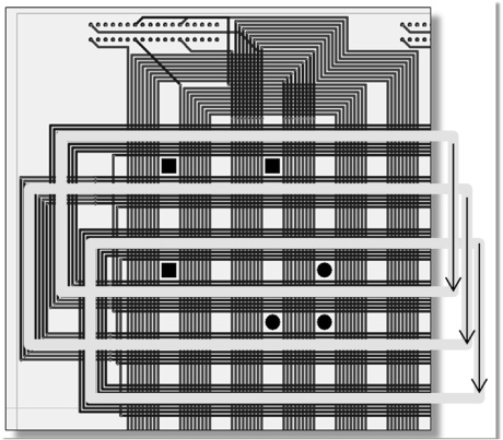
Therefore, the coil design was changed to a layout which is shown in Fig. 6. This design opens small gaps between the coils for the sensors. The disadvantage is that the linear properties of the force generation are disturbed a little and the efficiency is lower than before.

3.Linearization of lifting and X/Y forces

The idea is to use a thin incremental encoder glass below the movable stage and above the coils. (see figure7) Small gaps have to be placed between the driving coil layout for access to the sensor heads. However, the gaps cause distortions in linear force generation.

Fig. 7.

Magnetic flux, the location of the 2-D sensor grid and 3-phase coil arrangement for one of the 8 Halbach arrays, the magnetic flux is going thru the sensor grid.

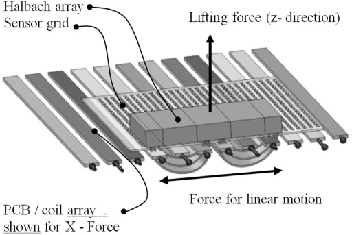
Fig. 8.

Cut view in 2D through the Halbach array and coils with the magnetic lines for a configuration without gaps between the 3-phase coils, but this does not allow sensor access through the PCB.

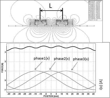
Fig. 9.

Gaps of 4 mm are between the 3-phase coil structure, 2-D view on a cut of only one of the Halbach array and the corresponding coils.

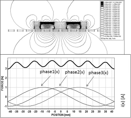
It can be shown that the horizontal component can also be decoupled and linearized by using a spatial frequency phase shift between two phases. It was explained in the article [6]. With this feed forward term, the control function can be linearized despite the fact that the gaps in the coil structure distort the linear properties. Figure 8 shows the force distrubution without gaps in the coil structure and figure 9 shows the larger distrution with the required gaps.

The spacial frequency can be extracted from the magnet structure geometry with half wavelength L = 𝜆 ∕2 = 42 mm. The following formula describes the phase condition for the driving current for a lifting force (force in Z-direction dependent from the linear position x):

The force ripple over position can be reduced by pre-shaping the driving current spatial frequency (position-dependent current). With dependent amplitude ampl (x) the 3 phase currents can be modified to reduce the force ripple.

Superposition of the 3-phase / 60 deg current through the coils for the lifting force (z force) with a spatial modulation to cancel the nonlinearities. The decreasing of the lifting force on the left and right side in Fig. 10 is because of the limited range of the coil in the simulation. A small part of the magnetic field does not interact with the coils on the left and right side because of the limited length in the simulation. (60-degree, 3-phase coil period is 84 mm).

Fig. 10.

Cut view in 2D through one Halbach array and coils (PCB) with the magnetic lines for a configuration with gaps between the 3-phase coils.

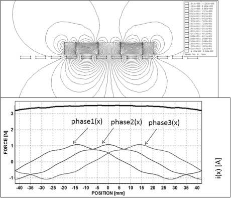
Fig. 11.

Current distribution of one phase of the drivers over the motion range of the planar stage.

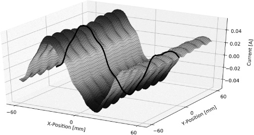
With a 3-D force measurement method a more detailed current 3-phase distribution can be shown in Fig. 11. The diagram shows about the same shaping (see on a cut in the X-Y plane) like the simple 2-D simulation has shown [6].

4.2-D sensor grid and measurement

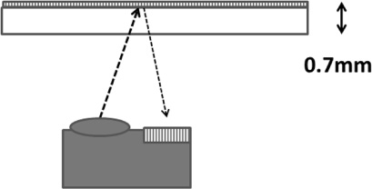
The sensor grid is on a 0.7 mm hardened glass plate which is mounted on tiny walls between the 4 Halbach arrays. The reflective grid dots are placed on the upper side of the glass plate. The light from the LED of the small incremental sensor heads has to cross the tiny glass plate and it is reflected onto the chromium dots, quasi on the “rear side” of the glass. The other area around the dots is black to absorb the LED light with a wavelength of 650 nm. (see figure 12)

Fig. 12.

Principle of incremental sensor heads, the grid on the sensor head and the grid on the movable stage produce a Moiré effect on the photodiode receivers.

A set of 4 pieces of such incremental sensor heads (figure 13) is used to detect the X, Y, and rotation around the vertical axis 𝜑Z = 𝛼 of the grid (stage). Two heads are placed in the X direction, two are placed in the Y direction. The use of this four-head configuration (three heads are necessary for the detection of the 3 DOF) offers an addition redundancy. (see figure 14)

Fig. 13.

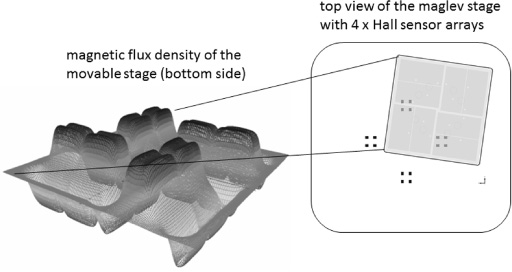
Arrangement of the 4 optical incremental sensor heads to detect the X, Y, and rotation around the vertical axis.

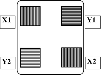
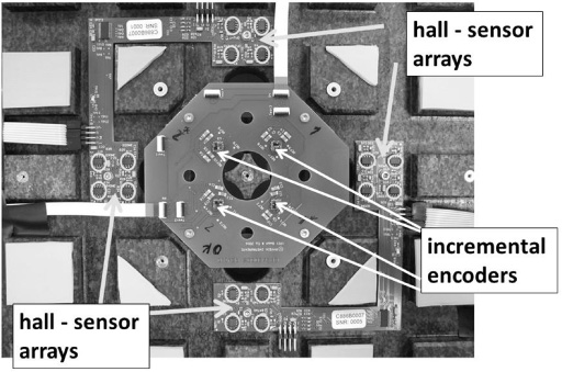
Fig. 14.

Image of the 4 incremental encoders below the main coil PCB. Four hall-arrays consisting of 4 sensors each are used around the incremental heads for detecting the initial position of the stage.

The angular position is calculated by the position differences D and the mechanical distance of the sensor heads.

It is recommended to use ceramic PCB material for better thermal stability of the distance between the sensor heads. The board is fixed in the middle and is “swimming” and stabilized with flexible adhesives on the four corners.

Fig. 15.

Motion controller structure for magnetic levitation stage.

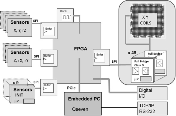
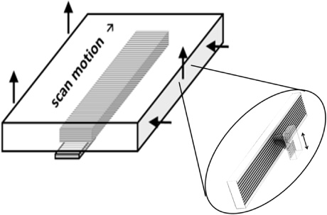
Fig. 16.

Linear maglev system can only use grid sensors (arrows show the measurement direction), a long scale is used for the motion detection sensor in the scan direction.

The lower surface of the glass plate is used to detect the flight height of the 2-D sensor grid. The flight height is detected with distance sensors using a 1550 nm wavelength. Therefore, on the lower side of the glass plate a sputtered filter is placed consisting of dielectric layers that reflect the 1550 nm and transmit the 650 nm of the X Y 𝜑Z sensors. (xs, ys, 𝛼).

5.Motion controller

All types of high-precision magnetic levitation systems need a vector-controlled complex controller. The control loops over the three forces and three torque components have to be closed by high servo rate. In our example, the controller needs access to 23 sensors and 24 coil drivers (6 of the 144 coils are connected serial/ parallel and that results in at least to 24 independent controlled coils). (see figure15)

To control all types of the maglev systems in 6DOF, we developed a Q7-Intel multi-core based controller. The Q7 PC platform has a standardized size of 70 × 70 mm. Only low-level digital control signals are used between the controller and the maglev system. The sensors including interpolation units and the digital driven coil driver are close to the maglev system unit. The robust interface allows access and buffering of the sensor values and driver data in each 20 kHz control loop cycle. The interface is based on PCI express (peripheral component interconnect) with direct memory access bus mastering. With this data transfer technology, the computing power of the multi-core processor platform is not limited. The coil drivers run with 400 kHz PWM signals. This structure makes it easy to adapt the controller to any type of planar/linear or gantry maglev system.

Fig. 17.

Gantry maglev system can only use encoder sensors, (arrows show the measuring direction).

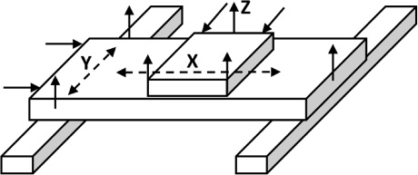
Fig. 18.

Magnetic flux density distribution on the bottom side of the movable platform with the Halbach arrays.

6.Linear magnetic levitation stage and gantry systems with 6 DOF

Linear magnetic levitation stages can be used for extremely precise scan and long term (no abrasion) applications where the out-of-plane motion needs to be minimized. Because the motion is controlled via precision sensors and is not influenced by inaccurate guiding, the motion can be controlled without any hysteresis effect. The sensors have to be aligned to the motion platform so that all 6 degrees of freedom can be detected independently for each degree of freedom. In the linear maglev design, there is no need for coil current pre-shaping and expensive interferometers. Finally, 5 degree of freedom should be “detected” and stabilized while one degree of freedom (the scan direction) is controlled over the long range. (figure 16) A large number of high-resolution incremental encoders are available. An encoder based on absolute measurement technology can also be used for the long stroke. One example of a high-resolution absolute encoder is provided by Renishaw’s type “RESOLUTE^TM”.

At least 5 encoder sensors can be used for detecting 5 degrees of freedom. The 5 encoders should have a short sensing range of 0.1 … 3 millimeters – depending on the control capability for the out-of-plane motion or additional features regarding angular settings. The sixth encoder is in the scan control loop and it is used to perform the tracking capability.

In maglev systems with a large scan range, larger than the length of the movable stage - the sensor heads have to be placed at the stage and the scale has to be placed at the support parts on the ground. This requires a cable trace or wireless transfer of the sensor data to the ground-based controller. In respect of this requirement, new wireless transfer of the sensor data is necessary. Wireless energy transmission will also be the main challenge in gantry systems (figure 17) otherwise the main advantage of friction and abrasion-free motion is infringed.

Only grid sensors can also be used also for gantry systems with a motion range larger than the size of the positioning stage.

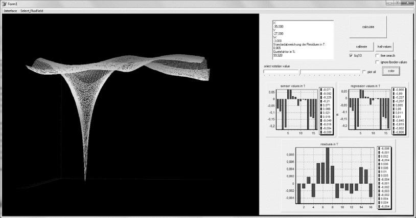
Fig. 19.

Software tool to calculate the correlation-fitting function on an array of positions.

7.Initialization sensors

There are a large number of incremental encoders, but not many absolute-measuring- encoders on the market. Some of them are very robust and much cheaper than absolute- measuring sensors. These nanometer-resolution sensors need a referencing procedure. We can show that 4 arrays of four Hall sensors can be used for the initialization procedure. (see figure 18) During this procedure, the system should be lifted without scratching the surface to prevent abrasion.

Figure 19 shows the correlation fitting function for the Halbach array position in relation to the 4 times 4 analog Hall sensors. The small peak (in this example) shows that for each position only one low error–solution is available. The method leads to unequivocal positions.

8.Conclusion

The paper describes new magnetic levitation systems with nanometer resolution, passive platforms with focus on cost-effective sensors and driver design. The system combines a fully passive stage with 8 Halbach arrays and an optical sensor grid. The optical incremental sensor grid is placed onto the movable stage between the magnetic arrays and the coil board, which is placed on a granite baseplate. 7 optical incremental sensors heads, and 4 times 4 analog Hall sensor arrays are fixed on the lightweight granite base.

It would be possible to use only linear incremental optical encoders in linear scan stages and also in gantry systems. This opens cost efficient designs for industrial applications. The magnetic levitation technology will solve the problems of abrasion in long-term scan applications.

References

[1] | W. Kim and D. Trumper, High-precision magnetic levitation stage for photolithography, Precision Eng. 22: (2) ((1998) ), 66–77. |
[2] | X. Lu and I. Usmann, A novel long stroke planar motor, Proc. ASPE ((2011) ), 3313. |
[3] | P. Frissen, J. Compter, M. Renkens, G. Fockert and R. Coolen, US Patent 6,847,134, Displacement device, Jan. 25, 2005. |
[4] | R. Gloess, Ch. Mock, Ch. Rudolf, C. Walenda, Ch. Schaeffel, M. Katzschmann and H.-U. Mohr, Magnetic levitation in 6-DOF with Halbach array configuration, in: ACTUATOR, Bremen, (2010) . |
[5] | C. Schaeffel, M. Katzschmann, H. Mohr, R. Gloess, C. Rudolf, C. Mock and C. Walenda, Planar magnetic levitation system PIMag 6D, JSME Journal Vol 3: (No 1) ((2016) ), 1–7. |
[6] | R. Gloess, Mag-6D a new mechatronics design of a levitation stage with nanometer resolution, in: ASPE Proceedings, Portland, (2016) , pp. 423–427. |
[7] | R. Gloess and A. Goos, 6-DOF force measurement platform used for mapping functions in magnetic levitation systems, in: ASPE Proceedings, Las Vegas, (2018) . |