Abstract
For several different boundary conditions (Dirichlet, Neumann, Robin), we prove norm-resolvent convergence for the operator −Δ in the perforated domain Ω∖⋃i∈2εZdBaε(i), aε≪ε, to the limit operator −Δ+μι on L2(Ω), where μι∈C is a constant depending on the choice of boundary conditions.
This is an improvement of previous results [Progress in Nonlinear Differential Equations and Their Applications 31 (1997), 45–93; in: Proc. Japan Acad., 1985], which show strong resolvent convergence. In particular, our result implies Hausdorff convergence of the spectrum of the resolvent for the perforated domain problem.
1.Introduction
In this article we study the following homogenisation problems labelled by ι∈{D,N,α} (“D” for Dirichlet, “N” for Neumann, and “α” for Robin). Let Ω⊂Rd, d⩾2 be open (bounded or unbounded) with C2 boundary. For unbounded domains Ω we assume translation invariance, i.e., Ω+z=Ω for any z∈Zd. Let α∈C∖{0},Re(α)⩾0 and denote Ωε:=Ω∖⋃i∈LεBaε(i) where ε∈(0,1), Baε(i) is the ball of radius
(1.1)aεD=εd/(d−2),d⩾3,e−1/ε2,d=2,aεN=o(ε)(ε→0),aεα=εd/(d−1)
centered at the point
i∈Lε, and
(1.2)Lε:={i∈2εZd:dist(i,∂Ω)>ε}.
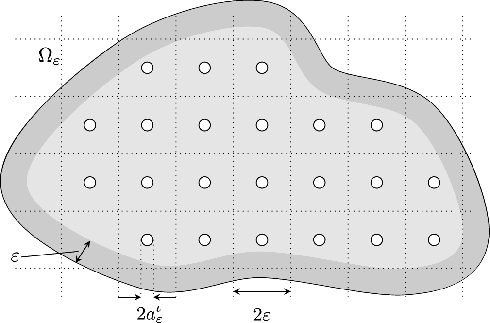
Consider the boundary value problems (cf. Figure 1)
(Dir)(−Δ+1)uε=fin Ωε,uε=0on ∂Ωε,(Neu)(−Δ+1)uε=fin Ωε,∂νuε=0on ∂Ωε,(Rob)(−Δ+1)uε=fin Ωε,∂νuε+αu=0on ∂Ωε,
i.e. the resolvent problem for the Laplacian, subject to the Dirichlet, Neumann and Robin boundary conditions, respectively. It is easy to see, using the Lax–Milgram theorem, that for all
ε∈(0,1) each of these problems has a unique weak solution
uε. It is a classical question, which we refer to as the homogenisation problem, whether the family of solutions to (
Dir), (
Neu), (
Rob), obtained by varying the parameter
ε, converges in the sense of the
L2-norm to a function
u∈L2(Ω) as
ε→0 and whether the limit function
u solves, in a reasonable sense, some PDE whose form is independent of the right-hand side datum
f.
Fig. 1.
Sketch of the perforated domain.
Homogenisation problems of this type have been studied extensively for a long time [2,5,7,11]. For example, results by Cioranescu & Murat and Kaizu give a positive answer to the previous question for all three choices of boundary conditions at least in the case of bounded domains. In fact, they showed that the solutions of (Dir), (Rob), (Neu) converge strongly in L2(Ω) to the solution u∈H1(Ω) of (−Δ+1+μι)u=f, where
(1.3)μι=π2,ι=D,d=2,(d−2)Sd2d,ι=D,d⩾3,0,ι=N,αSd2d,ι=α,
where
Sd denotes the surface area of the unit ball in
Rd.
In this article we attempt to improve this result in two directions. First, we show the above convergence not only in the strong sense, but in the norm-resolvent sense (that is, the right-hand side f is allowed to depend on ε). Second, our result is then extended to the case of unbounded domains. As a corollary, we obtain a statement about the convergence of the spectra of the perforated domain problems (Dir), (Neu), (Rob) as ε→0.
The paper is organised as follows. In Section 2 we will briefly give a more precise formulation of the problem and include previous results. In Section 3 we will state our main result and its implications. Sections 4, 5 and 6 contain the proof of the main theorem and in Section 7 we consider implications of our main theorem for the semigroup generated by the Robin Laplacian. Section 8 contains a brief conclusion and discusses open problems.
2.Geometric setting and previous results
As above, assume d⩾2, and let
Tε:=⋃i∈LεTiε,Tiε:=Baει(i),i∈Lε,
where
aει,
Lε as in (
1.1), (
1.2). Denote
Ωε:=Ω∖Tε. We also denote
Biε:=Bε(i) and
Piε:=ε[−1,1]d+i for
i∈Lε. Constants independent of
ε will be denoted
C and may change from line to line. Note that our assumptions on Ω ensure that the set
{ϕ|Ω:ϕ∈C0∞(Rd)} is dense in
H1(Ω) (cf. [
1, Cor. 9.8]) in the cases
ι=N,α.
Moreover, since we are dealing with varying spaces L2(Ωε), it is convenient to define the identification operators
(2.1)Jε:L2(Ωε)→L2(Ω),Jεf(x)=f(x),x∈Ωε,0,x∈Ω∖Ωε(2.2)Iε:L2(Ωε)→L2(Ω),Iεg(x)=g|Ωε(2.3)Tε:H1(Ωε)→H1(Ω),Tεu=u in Ωε,v in Tε,
where
v is the harmonic extension of
u into the holes, i.e.
(2.4)Δv=0in Tε,v=uon ∂Tε.
Lemma 2.1.
For Iε,Jε as above, one has
(2.5)IεJε=idL2(Ωε)(2.6)‖JεIε−idL2(Ω)‖L(H1(Ω),L2(Ω))→0.
Moreover, ‖Iε‖L(L2(Ωε),L2(Ω)),‖Jε‖L(L2(Ω),L2(Ωε)) are uniformly bounded in ε.Proof.
The only nontrivial statement is (2.6). To prove this, let f∈H1(Ωε). Then ‖f−JεIεf‖L2(Ω)=‖f‖L2(Tε). To show that this quantity converges to 0 uniformly in f, denote Qk:=[0,1)d+k for k∈Zd a cube shifted by k, so that Rd=⋃k∈ZdQk. Then we have
‖f‖L2(Tε)2=∑k∈Zd‖f‖L2(Qk∩Tε)2⩽∑k∈Zd‖1‖L2p(Qk∩Tε)2‖f‖L2q(Qk∩Tε)2
for
p,q>1 with
p−1+q−1=1, by Hölder’s inequality. Since
f∈H1(Ω), we can use the Gagliardo–Sobolev–Nierenberg inequality to conclude (for suitable
q) that
‖f‖L2(Tε)2⩽‖1‖L2p(Q0∩Tε)2∑k∈Zd‖f‖L2q(Qk∩Tε)2⩽‖1‖L2p(Q0∩Tε)2∑k∈ZdC‖f‖H1(Qk∩Tε)2=|Q0∩Tε|1/pC‖f‖H1(Tε)2
with some suitable
p>0. Since
|Q0∩Tε|→0 as
ε→0 (cf. the definition of
aει, (
1.1)), the desired convergence follows. □
Lemma 2.2.
In the cases ι∈{N,α} the harmonic extension operator Tε satisfies
(i) lim supε→0‖Tε‖H1(Ωε)→H1(Ω)<∞.
(ii) There exists C>0 such that ‖Tεw‖H1(Piε)⩽C‖w‖H1(Piε) for all w∈H1(Ωε) and i∈Lε.
(iii) For any sequence wε such that lim supε→0‖wε‖H1(Ωε)<∞ one has ‖Tεwε−Jεwε‖L2(Ω)→0.
Proof.
See [5], [11, p. 40]. □
In the above geometric setting, we will study the linear operators Aει, ι=D,N,α in L2(Ωε), defined by the differential expression −Δ+1, with (dense) domains
D(AεD)=H01(Ωε)∩H2(Ωε),D(AεN)={u∈H2(Ωε):∂νu=0 on ∂Ωε},D(Aεα)={u∈H2(Ωε):∂νu+αu=0 on ∂Ωε},
respectively, and the linear operators
Aι in
L2(Ωε) defined by the expression
−Δ+1+μι, with domains
D(AD)=H01(Ω)∩H2(Ω),D(AN)={u∈H2(Ω):∂νu=0 on ∂Ω},D(Aα)={u∈H2(Ω):∂νu+αu=0 on ∂Ω},
respectively, where
μι,
ι=D,N,α, are defined in (
1.3).
Remark 2.3.
In the case when d⩾3 one has the characterisation
(2.7)μD=12dmin{∫Rd∖B1(0)|∇u|2,u∈H1(Rd),u=1 on B1(0)}.
Note that the factor
1/2d arises from the fact that the unit cell is of size
2ε.
Using the notation above, we recall the following classical results.
Theorem 2.4
Theorem 2.4([2]).
Let Ω⊂Rd be open (bounded or unbounded). Suppose that f∈L2(Ω), and let uε and u˜ be the solutions to
(−Δ+1)uε=f,uε∈H01(Ωε),(−Δ+1+μD)u˜=f,u˜∈H01(Ω).
Then Jεuε⇀ε→0u˜ in H01(Ω).Theorem 2.5
Theorem 2.5([5]).
Let Ω⊂Rd be open (bounded or unbounded), and suppose that ∂Ω is smooth. Suppose also that f∈L2(Ω), and let uε and u˜ be the solutions to
(−Δ+1)uε=f,uε∈D(Aεα,N),(−Δ+1+μα,N)u˜=f,u˜∈D(Aα,N).
Then one has
Jεuε⇀ε→0u˜in H1(Ω).
Proof of Theorems 2.4and 2.5.
The results are obtained by following the proofs of [2, Thm 2.2], [5, Thm 2]. Note that the weak convergence in H1(Ω) is immediately obtained also for unbounded domains (and complex α). □
An important ingredient in the proofs are auxiliary functions wϵι∈W1,∞(Rd) defined, for each ε∈(0,1), as the solution to the problems
(2.8)wεN≡1,wεD=0in Tiε,ΔwεD=0in Biε∖Tiε,wεD=1in Piε∖Biε,wεDcontinuous,∂νwεα+αwεα=0on ∂Tiε,Δwεα=0in Biε∖Tiε,wεα=1in Piε∖Biε,wεαcontinuous,
used as a test function in the weak formulation of the problems (
Dir), (
Neu), (
Rob).
These functions were used in [2,5] as test functions to prove strong convergence of solutions. They are “optimal” in the sense that they minimise the energy in annular regions around the holes. In the Dirichlet case, the function wεD is nothing but the potential for the capacity cap(Bε(i);BaεD(i)). It can be shown that one has the convergences
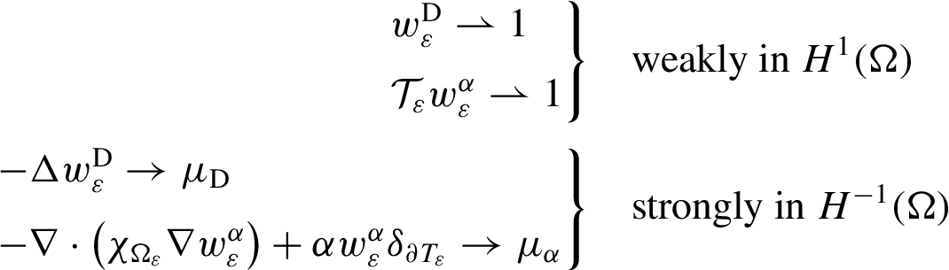
as ε→0, where δ∂Tε denotes the Dirac measure on the boundary of the holes (for a proof of the above facts, see [2, Lemma 2.3] and [5, Section 3]).
3.Main results
In what follows we prove the following claim.
Theorem 3.1.
Let Jε,Aει,Aι be defined as in the previous section. Then for ι∈{D,N,α} one has
(3.1)‖Jε(Aει)−1−(Aι)−1Jε‖L(L2(Ωε),L2(Ω))→0(ε→0),
that is, the operator sequence Aει converges to Aι in the norm-resolvent sense.Corollary 3.2.
If Aε,A are as in Theorem 3.1, then
(3.2)‖(Aει)−1Iε−Iε(Aι)−1‖L(L2(Ω),L2(Ωε))→0,
where Iε is as in (2.2).Proof.
For notational convenience, denote Rε:=(Aει)−1 and R:=(Aι)−1. A quick calculation shows that
RεIε−IεR=Iε(JεRε−RJε)Iε−(IεJε−1)RεIε=Iε(JεRε−RJε)Iε,
since
IεJε=idL2(Ωε). Hence
‖RεIε−IεR‖L(L2(Ω),L2(Ωε))⩽‖Iε‖L(L2(Ω),L2(Ωε)2‖JεRε−RJε‖L(L2(Ωε),L2(Ω))→0
as
ε→0, by (
3.1) and uniform boundedness of
‖Iε‖L(L2(Ωε),L2(Ω)). □
We note an important consequence of the above theorem.
Corollary 3.3.
For all compact K⊂C, one has σ(Aει)∩K→ε→0σ(Aι)∩K in the Hausdorff sense.11
Proof.
First, note that the spectra of Aει converge to that of Aι, in the sense that for each compact K⊂ρ(Aι) there exists ε0>0 such that K⊂ρ(Aει) for all ε∈(0,ε0). The proof of this is obtained by combining the proofs of Lemma 3.11, Theorem 3.12 and Corollary 3.14 in [8]. On the other hand, an analogous proof using (3.2) and (2.6) shows that if K⊂ρ(Aει) for almost all ε>0, then K⊂ρ(Aι). Together these two facts imply Hausdorff convergence. □
In particular, this corollary shows that (if Re(μι)>0) a spectral gap opens for Aει between 0 and Re(μι).
Remark 3.4.
We note that our assumption on the spherical shape of the holes was made for the sake of definiteness, however, our results easily generalise to more general geometries as detailed in [2, Th. 2.7]. Moreover, our results are also valid for more general elliptic operators div(A∇) with continuous coefficients A (cf. [2]).
4.Uniformity with respect to the right-hand side
In this section we prove that the result of Theorems 2.4, 2.5 hold in a strengthened form, namely, uniformly with respect to the right-hand side f. More precisely, the following holds.
Theorem 4.1.
Suppose that εn↘0, fn∈L2(Ωεn), n∈N, with ‖fn‖L2(Ωε)⩽1, and let unι and u˜nι be the solutions to the problems (ι∈{D,N,α})
(4.1)(−Δ+1)unι=fn,unι∈D(Aεnι),(4.2)(−Δ+1+μι)u˜nι=Jεnfn,u˜nι∈D(Aι).
Then for every bounded, open K⊂Ω one has
Jεnunι−u˜nι→0strongly in L2(K),Jεn∇unι−∇u˜nι⇀0weakly in L2(K),
for ι∈{D,N,α}.Proof.
We have the following a priori estimates (note Lemma 2.2):
‖Tεnunα,N‖H1(Ω)⩽C‖Jεnfn‖L2(Ω),‖JεnunD‖H1(Ω)⩽C‖Jεnfn‖L2(Ω),‖u˜nι‖H1(Ω)⩽C‖Jεnfn‖L2(Ω)∀ι∈{D,N,α}.
Thus, there exists a subsequence (still indexed by
n) and
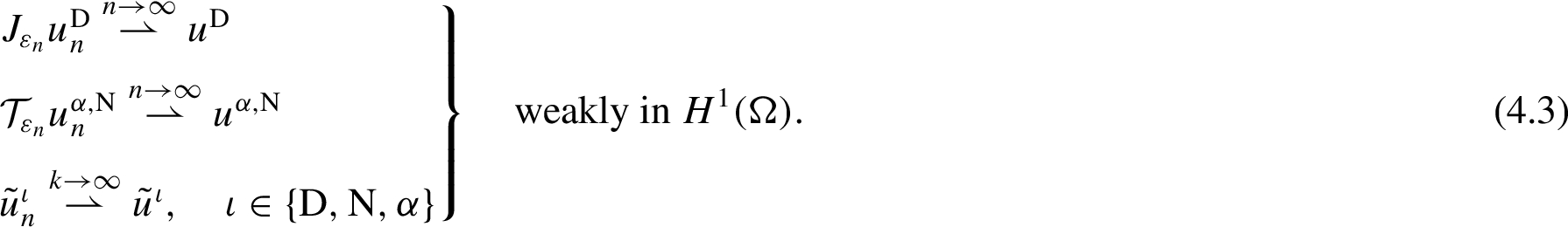
uι,u˜ι∈H1(Ω) such that
Note that that for every bounded K⊂Ω the convergence statements (4.3) are strong in L2(K). In particular, employing Lemma 2.2(i), (iii) and the Rellich Theorem we immediately obtain
Jεnunι→uιstrongly in L2(K),Jεn∇unι⇀∇uιweakly in L2(K)(4.4)u˜nι⇀u˜ιstrongly in L2(K),(4.5)∇u˜nι⇀∇u˜ιweakly in L2(K).
for all
ι∈{D,N,α}. Next, choose a further subsequence (still indexed by
n) such that also
Jεnfn⇀n→∞f weakly in
L2(Ω), where the limit
f may depend on the choice of subsequence. Now, consider the weak formulations of the problem (
4.2),
i.e.
∫Ω∇u˜nι‾∇ϕ+(1+μι)∫Ωu˜nι‾ϕ=∫Ωfn‾ϕ,
where
ϕ∈C0∞(Ω) for
ι=D and
ϕ∈C0∞(Rd) for
ι=α,N. Letting
n→∞ and using the convergencies (
4.4), (
4.5) (with
K=Ω∩suppϕ) we obtain
∫Ω∇u˜ι‾∇ϕ+(1+μι)∫Ωu˜ι‾ϕ=∫Ωf‾ϕ.
Next consider the weak formulation of (
4.1),where we choose the test function
wεnιϕ:
∫Ωεn∇unι‾∇(wεnιϕ)+∫Ωεnunι‾wεnιϕ=∫Ωεnfn‾wεnιϕ,
where again
ϕ∈C0∞(Ω) for
ι=D and
ϕ∈C0∞(Rd) for
ι=α,N. It follows from the results of [
2,
5] that the left and right-hand side of this equation converge to
∫Ω(∇uι‾∇ϕ+(1+μι)uι‾ϕ)and∫Ωf‾ϕ,
respectively. Thus, we obtain
∫Ω(∇uι‾∇ϕ+(1+μι)uι‾ϕ)=∫Ωf‾ϕ,
and hence
uι and
u˜ι are weak solutions to the same equation. Uniqueness of solutions (for all
ι∈{D,N,α}) implies
u˜ι=uι, which shows the assertion for the chosen subsequence.
Finally, applying the above reasoning to every subsequence of (Jεnunι−u˜nι) yields the result for the whole sequence. □
Corollary 4.2.
If the domain Ω is bounded, one has
‖Jε(Aει)−1−(Aι)−1Jε‖L(L2(Ωε),L2(Ω))→0(ε→0)
for ι∈{D,N,α}, i.e., Theorem 3.1 holds in that case of bounded Ω
.Proof.
Since Ω is bounded, the embedding of H1(Ω) in L2(Ω) is compact, thus the sequence Jεnunι−u˜nι from the previous proof has a subsequence converging to 0 strongly in L2(Ω). Since this can be done for every subsequence of (Jεnunι−u˜nι), the whole sequence converges to 0.
Now, choose a sequence fn∈L2(Ωεn),‖fn‖L2(Ωε)⩽1, such that
supf∈L2(Ωεn)‖f‖⩽1‖(Jεn(Aει)−1−(Aι)−1Jεn)f‖L2(Ωε)−1n<‖(Jεn(Aεnι)−1−(Aι)−1Jεn)fn‖L2(Ωεn).
By the above, the right-hand side of this inequality converges to zero, which implies the claim. □
Treating unbounded domains requires further effort. Since we lack compact embeddings in this case, we will have to take advantage of the sufficiently rapid decay of solutions to (−Δ+1)u=f and a decomposition of the right hand side with a bound on the interactions.
5.Exponential decay of solutions
We begin with a general result which we assume is classical, but include for the sake of completeness. Let U⊂Rd open satisfying the strong local Lipschitz condition, λ>12 and consider the problems (cf. (Dir), (Neu), (Rob))
(5.1)(−Δ+λ)uα=fin U,∂νuα+αuα=0on ∂U;(5.2)(−Δ+λ)uN=fin U,∂νuN=0on ∂U;(5.3)(−Δ+λ)uD=fin U,uD=0on ∂U.
Let
x0∈Rd, and define the function
ω(x)=cosh(|x−x0|). Then the following statement holds.
Proposition 5.1.
Let f∈L2(U), supp(f) compact. Then each of the problems (5.1)–(5.3) has a unique weak solution uι∈H1(U) satisfying
(5.4)∫U|uι|2ωdx⩽M∫U|f|2ωdx(5.5)∫U|∇uι|2ωdx⩽M∫U|f|2ωdx,
where M:=max{2,(λ−12)−1}.We postpone the proof, in order to introduce some notation and prove auxiliary results. First, let us denote dμ:=ωdx and introduce the weighted Sobolev spaces H:=W1,2(U;ω), H0:=W01,2(U;ω) with scalar product
⟨u,v⟩H=∫Uuvdμ+∫U∇u·∇vdμ.
Moreover, let
λ>12 and define the sesquilinear forms
(5.6)aα(u,v):=∫U(∇u‾·∇v+λu‾v)dμ+∫Uv∇u‾·∇ωωdμ+α∫∂Uu‾vωdSon H,(5.7)aN(u,v):=∫U(∇u‾·∇v+λu‾v)dμ+∫Uv∇u‾·∇ωωdμon H,(5.8)aD(u,v):=∫U(∇u‾·∇v+λu‾v)dμ+∫Uv∇u‾·∇ωωdμon H0.
Lemma 5.2.
For λ>12 and ι∈{D,N,α}, the form aι is continuous and coercive on H (on H0 in the case ι=D).
Proof.
We will only treat the Robin case here, the other cases being analogous. Denote by I the second term in (5.6) and note that ω was chosen so that |∇ω|⩽ω. By Hölder’s inequality with respect to μ one has
|I|⩽‖∇ωω‖∞︸⩽1‖∇u‖L2(μ)‖v‖L2(μ)⩽12‖∇u‖L2(μ)2+12‖v‖L2(μ)2,
and thus
|a(u,u)|⩾‖∇u‖L2(μ)2+λ‖u‖L2(μ)2+|α|‖ω1/2u‖L2(∂U)2+I⩾‖∇u‖L2(μ)2+λ‖u‖L2(μ)2−12‖∇u‖L2(μ)2−12‖u‖L2(μ)2=12‖∇u‖L2(μ)2+(λ−12)‖u‖L2(μ)2,
which shows coercivity in
H. Continuity follows by estimating the boundary term. By the trace theorem [
3, Prop. IX.18.1] we have, for each
δ>0,
(5.9)∫∂U|u|2ωdx⩽2δ‖∇(ω1/2u)‖L2(U)2+Cδ‖ω1/2u‖L2(U)2.
The first term can be estimated using the special choice of
ω:
‖∇(ω1/2u)‖L2(U)2=∫U|ω1/2∇u+12u∇ωω1/2|2dx⩽2∫Uω|∇u|2dx+12∫U|u|2|∇ω|2ωdx⩽2‖∇u‖L2(μ)+2‖∇ωω‖∞2∫U|u|2ωdx(5.10)⩽2‖∇u‖H1(μ)2.
The desired continuity now follows immediately by combining (
5.9) and (
5.10). □
Lemma 5.3.
Let f∈L2(U), ι∈{D,N,α}, and suppose that supp(f) is compact. Then the problem
(5.11)aι(u,v)=∫Uf‾vdμ∀v∈H
has a solution in H.Proof.
By Hölder inequality, one has
|∫Uf‾vdμ|⩽‖f‖L2(μ)‖v‖L2(μ)⩽‖ω‖L∞(suppf)‖f‖L2(U)‖v‖L2(μ),
so
f∈H′. The assertion now follows from Lemma
5.2 and the Lax–Milgram theorem for complex, non-symmetric sesquilinear forms [
13, Thm. VI.1.4]. □
Proof of Proposition 5.1.
Again we focus on the Robin case, the other cases being analogous. Denote by u the solution obtained from Lemma 5.3. Then u∈H1(U), since H⊂H1(U). Moreover, let ϕ∈C0∞(Rd) be arbitrary and decompose it as ϕ=ωψ. Then ψ∈C0∞(Rd)⊂H and one has
∫U∇u‾·∇ϕdx+λ∫Uu‾ϕdx+α∫∂Uu‾ϕdS=∫U∇u‾·(ω∇ψ+ψ∇ω)dx+λ∫Uu‾ψωdx+α∫∂Uu‾ψωdS=aα(u,ψ)=∫Uf‾ψdμ=∫Uf‾ϕdx.
Thus, the function
u solves the problem
(5.12)∫U∇u‾·∇ϕdx+λ∫Uu‾ϕdx+α∫∂Uu‾ϕdS=∫Uf‾ϕdx∀ϕ∈C0∞(Rd).
Uniqueness of solutions and density of
C0∞(Rd) in
H1(U) implies that
u is the weak solution in
H1(U) to the Robin problem (
5.1).
The estimates (5.4), (5.5) follow from the coercivity of aι. □
6.Decomposition of the right-hand side
In this section we consider the case of unbounded Ω. We conclude the proof of Theorem 3.1 by decomposing the domain into cubes Qi, writing f=∑ifχQi and then applying the above results to each term fχQi. The following lemma shows uniform convergence with respect to the position of the cubes.
Lemma 6.1.
Let εn↘0 and fn∈L2(Ω), n∈N, be such that ‖fn‖L2(Ω)⩽1 and supp(fn)⊂Qin, where Qin=[0,1]d+in with in∈Zd. Let unι,u˜nι be the solutions to the problems
(6.1)Aεnιunι=fn|Ωεn,Aιu˜nι=fn,n∈N,ι∈{D,N,α}.
Then ‖Jεnunι−u˜nι‖L2(Ω)→0 for all ι∈{D,N,α}.Proof.
The idea of the proof is to use translation invariance, in order to shift supp(fn) back near zero for every n, and then use the Fréchet–Kolmogorov compactness criterion to obtain a convergent subsequence of (Jεnunι−u˜nι); Theorem 4.1 will identify its limit as zero. Since the following analysis is independent of the choice of boundary conditions, we henceforth omit ι to simplify notation.
We now carry out the outlined strategy. We set, for all n∈N,
un∗(x):=un(x+in),u˜n∗(x):=u˜n(x+in),fn∗(x):=fn(x+in).
These functions still solve the problems (6.1) with fn replaced by fn∗ and Ω replaced by Ω−in. The new sequence fn∗ has the nice property that supp(fn∗)⊂[0,1]d for all n. In the following we consider Jεnun∗,u˜n∗,fn∗ as elements of L2(Rd) that are zero outside Ω−in. We will now show that u˜n∗−Jεnun∗ converges to zero in L2(Rd). To this end, consider the bounded set
(6.2)F:={u˜n∗−Jεnun∗:n∈N}⊂L2(Rd).
Claim: F is precompact in L2(Rd).
We postpone the proof of this claim to Lemma 6.2. We immediately obtain that (u˜n∗−Jεnun∗) has a convergent subsequence in L2(Rd). Furthermore, Theorem 4.1 shows that ‖u˜n∗−Jεnun∗‖L2(K)→0 for every bounded K⊂Rd which identifies the limit of the subsequence as zero.
Arguing as above for all subsequences of (u˜n∗−Jεnun∗), we conclude that u˜n∗−Jεnun∗→0 in L2(Rd). Since the shift u↦u(·+in) is an isometry in L2(Rd), this implies that u˜n−Jεnun→0 in L2(Ω). □
Lemma 6.2.
The set F defined in (6.2) is precompact in L2(Rd).
Proof.
We will use the notation and conventions from the previous proof and distinguish between the Dirichlet case and the Robin/Neumann cases.
Dirichlet case. Step 1: We have
supn‖τh(u˜n∗−Jεnun∗)−(u˜n∗−Jεnun∗)‖L2(Rd)→0as h→0∀n∈N,
where
τh denotes the operator of translation by
h. Indeed, the standard regularity theory implies
‖τh(u˜n∗−Jεnun∗)−(u˜n∗−Jεnun∗)‖L2(Rd)⩽‖∇(u˜n∗−Jεnun∗)‖L2(Rd)|h|⩽C‖fn‖L2(Ω)|h|.
Step 2: Notice that
supn‖u˜n∗−Jεnun∗‖L2(Rd∖BR(0))→0as R→∞,
due to the following estimate in which we set
ω0(x):=cosh(|x|).
‖u˜n∗−Jεnun∗‖L2(Rd∖BR(0))2⩽2‖u˜n∗ω0ω0−1‖L2(Ω∖BR(0))2+2‖Jεun∗ω0ω0−1‖L2((Rd∖BR(0))2⩽4M‖fn∗ω0‖L2(Rd)2‖ω0−1‖L∞(Rd∖BR(0))2Prop. 5.1⩽C‖fn‖L2(Ω)2exp(−R)
which completes Step 2. Applying the Fréchet–Kolmogorov theorem yields the precompactness of
F.
Neumann and Robin case. Here the strategy is the same, but matters are complicated by the fact that Jεnun∗ is not in H1(Rd). To show that F is precompact, we decompose elements in F as
u˜n∗−Jεnun∗=(u˜n∗−Tεnun∗)+(Tεn−Jεn)un∗,
define
F1:={u˜n∗−Tεnun∗:n∈N},
F2:={(Tεn−Jεn)un∗:n∈N} and show that
F1 and
F2 are precompact in
L2(Rd). We will begin by showing that
F1 is precompact. To this end, denote by
E:H1(Ω)→H1(Rd) an extension operator satisfying
Eu|Ω=u and
‖Eu‖H1(Rd)⩽C‖u‖H1(Ω) for all
u∈H1(Ω) (cf. Prop. VII.19.1 and Remark VII.19.2 in [
3]). Note that by translation invariance one has
Eτh=τhE and
(Eun)∗=E(un∗). We start by proving that
supn‖τhE(u˜n∗−Tεnun∗)−E(u˜n∗−Tεnun∗)‖2→0as h→0
This readily follows from the estimate
‖τhE(u˜n∗−Tεnun∗)−E(u˜n∗−Tεnun∗)‖L2(Rd)⩽‖∇E(u˜n∗−Tεnun∗)‖L2(Rd)|h|⩽C‖u˜n∗−Tεnun∗‖H1(Ω+in)|h|⩽C‖fn∗‖L2(Ω+in)|h|⩽C|h|.
Next we prove that
supn‖E(u˜n∗−Tεnun∗)‖L2(Rd∖BR(0))→0as R→∞.
Indeed, notice first that
‖E(u˜n∗−Tεnun∗)‖L2(Rd∖BR(0))2⩽C(‖u˜n∗‖L2((Ω−in)∖BR(0))2+‖Tεnun∗‖L2((Ωεn−in)∖BR(0))2)(6.3)=C(‖u˜n‖L2(Ω∖BR(in))2+‖Tεnun‖L2((Ωεn)∖BR(in))2),
To treat the two terms on the right-hand side we apply Lemma
2.2(ii) and Proposition
5.1 with
ωin(x)=cosh(|x+in|) as follows. For the second term in (
6.3), we obtain
‖Tεnun‖L2(Ωεn∖BR(in))⩽C(‖un‖L2(Ω∖BR/2(in))+‖∇un‖L2(Ω∖BR/2(in)))⩽‖ωin1/2ωin−1/2un‖L2(Ω∖BR/2(in))+‖ωin1/2ωin−1/2∇un‖L2(Ω∖BR/2(in))⩽C(‖ωin1/2un‖L2(Ω∖BR/2(in))+‖ωn1/2∇un‖L2(Ω∖BR/2(in)))‖ωin−1/2‖L∞(Ω∖BR/2(in))⩽CM‖fnωin1/2‖L2(Ω)exp(−R/3)⩽2CMexp(−R/3),
where we use the fact that
ωin is bounded by 2 on
suppfn. With an analogous calculation for the first term in (
6.3), we finally find
(6.4)‖E(u˜n∗−Tεnun∗)‖L2(Rd∖BR(0))⩽Cexp(−R/3),
with
C independent of
n. Applying the Fréchet–Kolmogorov theorem yields the precompactness of the set
{E(u˜n∗−Tεnun∗):n∈N}. Finally, noting that
F1={E(u˜n∗−Tεnun∗):n∈N}χΩ and that multiplication by
χΩ is a bounded operator on
L2(Rd) we obtain precompactness of
F1.
To prove precompactness of F2, first note that by Lemma 2.2(iii) for any δ>0 there exists a n0 such that
‖(Jεn−Tεn)un∗‖2<δ∀n>n0.
Let us fix arbitrary
δ>0 and
n0 as above. It remains to estimate the terms
‖τh(Jεn−Tεn)un∗−(Jεn−Tεn)un∗‖L2(Rd),n⩽n0,
but these are only finitely many, which clearly converge to zero individually, and hence
supn⩽n0‖τh(Jεn−Tεn)un∗−(Jεn−Tεn)un∗‖2→0as h→0
Altogether we have shown that
supn‖τh(Jεn−Tεn)un∗−(Jεn−Tεn)un∗‖L2(Rd)=max{supn⩽n0‖τh(Jεn−Tεn)un∗−(Jεn−Tεn)un∗‖2,2δ}→h→02δ.
Since
δ>0 was arbitrary we finally get
limh→0supn∈N‖τh(Jεn−Tεn)un∗−(Jεn−Tεn)un∗‖L2(Rd)=0.
This completes the first Fréchet–Kolmogorov-condition. The proof of the second condition
supn‖(Jεn−Tεn)un∗‖L2(Rd∖BR(0))→0as R→∞
is analogous to the case of
F1. Applying the Fréchet–Kolmogorov theorem yields precompactness of
F1 and completes the proof. □
Corollary 6.3.
There exists δε with δε⟶ε→00 such that
‖(Jε(Aι)−1−(Aει)−1Jε)(fχQi∩Ωε)‖L2(Ω)⩽δε‖fχQi‖L2(Ω)
for all f∈L2(Ω) and i∈Zd.Proof.
We argue by contradiction. Suppose that there is no such function δε. Then there exist sequences εn,fn,in with ‖fn‖L2(Ω)=1 such that ‖(Jε(Aι)−1−(Aεnι)−1Jε)(fnχQin∩Ωεn)‖L2(Ω) does not converge to zero, which is a contradiction to Lemma 6.1. □
In order to finalise the decomposition, we require he following two lemmas.
Lemma 6.4.
Suppose that f∈L2(Ω), and denote
ui:=(Jε(Aι)−1−(Aει)−1Jε)(fχQi∩Ωε),i∈Zd.
Then one has
(6.5)|⟨ui,uj⟩L2(Ω)|⩽C‖fχQi‖L2(Ω)‖fχQj‖L2(Ω)exp(−|i−j|/2)
for all i,j∈Zd with i≠j, where ⟨·,·⟩L2(Ω) denotes the standard inner product in L2(Ω).Proof.
For convenience we write fi:=fχQi, i∈Zd. Denote ωi(x)=cosh(|x−i|) and note that by Proposition 5.1 we have ‖ωi1/2ui‖L2(Ω)⩽C‖fiωi1/2‖L2(Ω). The statement of the lemma is a consequence of the following estimate:
|⟨ui,uj⟩L2(Ω)|⩽∫Ω|ui(x)||uj(x)|dx=∫Ω(|ui(x)|ωi1/2)(|uj(x)|ωj1/2)ωi−1/2ωj−1/2dx⩽‖uiωi1/2‖L2(Ω)‖ujωj1/2‖L2(Ω)‖ωi−1/2ωj−1/2‖L∞(Ω)⩽C‖fiωi1/2‖L2(Ω)‖fjωj1/2‖L2(Ω)‖ω0−1/2ωj−i−1/2‖L∞(Ω)⩽C‖fi‖L2(Ω)‖fj‖L2(Ω)exp(−|i−j|/2),
where we use the fact that
supp(fi)⊂Qi and
ωi|Qi⩽2. □
Lemma 6.5.
Suppose that f∈C0∞(Ωε) and define ui:=(Jε(Aει)−1−(Aι)−1Jε)(fχQi), i∈Zd. Then for every n>1 one has the inequality
(6.6)‖∑m=1Nuim‖L2(Ω)2⩽C(n3∑m=1N‖uim‖L2(Ω)2+‖f‖L2(Ωε)exp(−n/3)),
where N is the number of cubes such that Qik∩supp(f)≠∅, and C,n do not depend on N.Proof.
‖∑m=1Nuim‖L2(Ω)2⩽∑m,p=1N⟨uim,ujp⟩L2(Ω)=∑k=0∞(∑|i−j|∈[k,k+1)⟨ui,uj⟩L2(Ω))⩽∑k=0n(∑|i−j|∈[k,k+1)‖ui‖L2(Ω)‖uj‖L2(Ω))+∑k=n∞(∑|i−j|∈[k,k+1)⟨ui,uj⟩L2(Ω))⩽∑k=0n∑|i−j|∈[k,k+1)(‖ui‖L2(Ω)22+‖uj‖L2(Ω)22)+∑k=n∞(∑|i−j|∈[k,k+1)⟨ui,uj⟩L2(Ω))⩽∑k=0n∑m=1N(∑{j:|im−j|∈[k,k+1)}‖uim‖L2(Ω)2)+∑k=n∞(∑|i−j|∈[k,k+1)⟨ui,uj⟩L2(Ω))⩽C∑k=1nk2∑m=1N‖uim‖L2(Ω)2+∑k=n∞(∑|i−j|∈[k,k+1)⟨ui,uj⟩L2(Ω))(6.7)⩽Cn3∑m=1N‖uim‖L2(Ω)2+∑k=n∞(∑|i−j|∈[k,k+1)⟨ui,uj⟩L2(Ω)).
We now study the last term of (6.7). It follows from Lemma 6.4 that
|⟨ui,uj⟩L2(Ω)|⩽C‖fi‖L2(Ω)‖fj‖L2(Ω)e−12|i−j|.
Using this fact and fixing
k for the moment, we obtain
|∑|i−j|∈[k,k+1)⟨ui,uj⟩L2(Ω)|⩽C∑|i−j|∈[k,k+1)‖fi‖L2(Ω)‖fj‖L2(Ω)exp(−|i−j|/2)⩽C∑|i−j|∈[k,k+1)(‖fi‖L2(Ω)22+‖fj‖L2(Ω)22)exp(−|i−j|/2)⩽C∑m=1N‖fim‖L2(Ω)2k2exp(−k/2)=C‖f‖L2(Ω)2k2exp(−k/2)⩽C‖f‖L2(Ω)2exp(−k/2).
Summing this inequality from
k=n to infinity concludes the proof. □
Combining the above lemmas, we have the following quantitative statement.
Proposition 6.6.
Suppose that f∈C0∞(Ωε). Then for every n∈N,
‖(Jε(Aει)−1−(Aι)−1Jε)f‖L2(Ω)2⩽C(n3δε2+exp(−n/3))‖f‖L2(Ω)2
for some C>0, where δε was defined in Corollary 6.3.Proof.
We denote uiε:=(Jε(Aει)−1−(Aι)−1Jε)(fχQi), i∈Rd, and estimate
‖(Jε(Aει)−1−(Aι)−1Jε)f‖L2(Ω)2=‖∑m=1Nuimε‖L2(Ω)2Lemma 6.5⩽C(n3∑m=1N‖uimε‖L2(Ω)2+exp(−n/3)‖f‖L2(Ωε))Cor. 6.3⩽C(n3δε2∑m=1N‖fim‖L2(Ωε)2+exp(−n/3)‖f‖L2(Ωε))=C(n3δε2+exp(−n/3))‖f‖L2(Ω)2.
□
Proof of Theorem 3.1.
Let g∈L2(Ωε) with ‖g‖L2(Ωε)⩽1. Fix δ>0 and choose f∈C0∞(Ωε) such that ‖g−f‖L2(Ωε)2<δ and choose n∈N such that exp(−n/3)⩽δ. Now compute
‖(Jε(Aει)−1−(Aι)−1Jε)g‖L2(Ω)2⩽2‖(Jε(Aει)−1−(Aι)−1Jε)f‖L2(Ω)2+2‖(Jε(Aει)−1−(Aι)−1Jε)(g−f)‖L2(Ω)2⩽C((n3δε2+exp(−n/3))‖f‖L2(Ωε)2+‖Jε(Aει)−1−(Aι)−1Jε‖2︸bounded‖g−f‖L2(Ωε)2)⩽C(n3δε2+δ)‖g‖L2(Ωε)2+Cδ,
hence
sup‖g‖L2(Ωε)⩽1‖(Jε(Aει)−1−(Aι)−1Jε)g‖L2(Ω)2⩽Cn3δε2+Cδ+Cδ,
and therefore
lim supε→0‖(Jε(Aει)−1−(Aι)−1Jε)‖L(L2(Ωε),L2(Ω))2⩽Cδ.
Since
δ>0 is arbitrary, the result follows. □
7.Behaviour of the semigroup
In this section we want to give an application of Theorem 3.1. In particular, we focus on the non-selfadjoint operator Aα and study the large-time behaviour of its semigroup. In order to do this, we shall first study the numerical range of the Robin Laplacians more closely. In the remainder of this section, unless otherwise stated, the symbols ‖·‖ and ⟨·,·⟩ will denote the L2 (operator-) norm and scalar product, respectively, and the symbol Σθ denotes a sector of half-angle θ in the complex plane.
7.1.Decay of e−t(Aα−Id)
Let α∈C and assume Reα>0. We want to study the decay properties of the heat semigroup et(Δ−μα). To this end, let us denote by Bα:=Aα−Id the Robin Laplacian on Ω. It is our goal to derive estimates on the numerical range of Bα. Let u∈D(Bα)=D(Aα) and assume that ‖u‖L2(Ω)=1. Notice that
⟨Bαu,u⟩=∫Ω|∇u|2dx+μα∫Ω|u|2dx+α∫∂Ω|u|2dS=‖∇u‖2+μα+α‖u‖L2(∂Ω)2,
and therefore
Re⟨Bαu,u⟩⩾Reμα+Reα‖u‖L2(∂Ω)2,|Im⟨Bαu,u⟩|⩽|Imμα|+|Imα|‖u‖L2(∂Ω)2.
Now, let
λ∈(0,Reμα) and compute
|Im⟨(Bα−λ)u,u⟩|⩽|Imμα|+|Imα|‖u‖L2(∂Ω)2(7.1)=|Imμα|ReμαReμα+|Imα|ReαReα‖u‖L2(∂Ω)2.
Recall from Section
1 that
μα=αSd/2d and hence
|Imμα|/Reμα=|Imα|/Reα. Combining this with (
7.1), we obtain (cf. Figure
2)
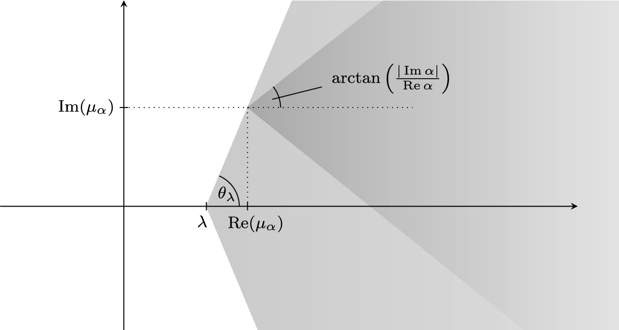
|Im⟨(Bα−λ)u,u⟩|⩽|Imα|Reα(Reμα+Reα‖u‖L2(∂Ω)2)⩽|Imα|Reα(Re⟨(Bα−λ)u,u⟩+λ)⩽|Imα|Reα−λ2−dSdRe⟨(Bα−λ)u,u⟩.
Fig. 2.
The sector of decay and angle θλ for Bα.
Using standard generation theorems about analytic semigroups, the next statement follows.
Proposition 7.1.
The operator −(Bα−λ) generates a bounded analytic semigroup in the sector Σπ2−θλ, where
θλ=arctan(|Imα|Reα−λ2−dSd).
Equivalently, −Bα generates an analytic semigroup with
‖exp(−zBα)‖⩽exp(−λz)∀z∈Σπ2−θλ.
Proof.
See [6, Ch. IX.1.6]. □
7.2.Decay of e−t(Aεα−Id)
In this section we denote Bεα:=Aεα−Id. By calculations analogous to the above, we have
|Im⟨Bεαu,u⟩|⩽|Imα|ReαRe⟨Bεαu,u⟩,
that is,
Bεα is sectorial with sector
Σθ0, where
θ0=arctan(|Imα|/Reα), and hence generates a bounded analytic semigroup in the sector
Σπ2−θ0. In this subsection we improve this
a priori result using spectral convergence. To this end, let
δ>0 and define the compact set
Kδ:={x+iy:x∈[0,Reμα],y∈[−|Imμα|,|Imμα|]}.
Note that then
Σθ0∩{Rez⩽Reμα−δ}⊂Kδ. By [
4, Th. III.2.3] one has
Kδ⊂ρ(Bα) for every
δ>0. Applying Corollary
3.3 we see that for every
δ>0 there exists a
ε0>0 such that
Kδ⊂ρ(Bεα) for all
ε<ε0.
In particular we have shown that the resolvent norm ‖(Bεα−z)−1‖ is bounded on Σθ0∩{Rez⩽Reμα−δ}. By a trivial calculation analogous to the previous subsection this leads to the following statement.
Lemma 7.2.
For every λ∈(0,Reμα−δ) one has
σ(Bεα−λ)⊂Σθλδ,θλδ=arctan(|Imμα|Reμα−λ−δ).
Furthermore, we obtain the following lemma.
Lemma 7.3.
For every λ∈(0,Reμα−δ) one has C∖Σθλδ⊂ρ(Bεα−λ) and there exists a M=M(λ,δ)>0 such that
‖(Bεα−λ−z)−1‖⩽M|z|∀z∈C∖Σθλδ.
Proof.
This is obtained by combining Lemma 7.2 with the following two facts:
|Im⟨Bεαu,u⟩|⩽|Imα|ReαRe⟨Bεαu,u⟩,‖(Bεα−z)−1‖⩽Con Kδ.
□
By the theory of analytic semigroups (cf. [6, Ch. IX.1.6]), we immediately obtain the following corollary.
Corollary 7.4.
For all λ∈(0,Reμα−δ), the operator Bεα−λ generates a bounded analytic semigroup in the sector Σπ2−θλδ.
This yields the main result of this section, as follows.
Theorem 7.5.
For every δ>0 there exists ε0>0 such that for every λ∈(0,Reμ−δ) there exists M>0 such that
‖exp(−zBεα)‖⩽Mexp(−λRez)∀z∈Σθλδ,ε∈(0,ε0).
Remark 7.6.
It is straightforward to repeat the above proof for the case of Dirichlet boundary conditions to obtain an analogous result for ‖exp(−t(AD−Id))‖. Here, the selfadjointness of AD allows us to choose the half-angle θ arbitrarily close to π/2.
8.Conclusion
We have shown norm-resolvent convergence in the classical perforated domain problem with Dirichlet boundary conditions which has the interesting implication of spectral convergence (Cor. 3.3). Some questions remain open and will be addressed in the future. While the norm ‖JεAε−1−A−1Jε‖L(L2(Ωε),L2(Ω)) converges to 0, it is not clear from our method of proof how fast this happens. It would be desirable to obtain a precise convergence rate. In the case of Dirichlet boundary conditions a explicit convergence rate has been found by [10]. Another interesting question is whether in the case Ω=Rd there exist gaps in the spectrum of Aε and how these depend on ε. The existence of spectral gaps has been confirmed in two dimensions [9], but to the authors’ knowledge the higher-dimensional case is still open.