A pseudo density topology optimization approach in nonlinear electromagnetism applied to a 3D actuator

Seebacher, Philipp; Kaltenbacher, Manfred; Wein, Fabian; Lehmann, Henry

doi:10.3233/JAE-201501

A pseudo density topology optimization approach in nonlinear electromagnetism applied to a 3D actuator

Article type: Research Article

Authors: Seebacher, Philipp^a; | Kaltenbacher, Manfred^b | Wein, Fabian^c | Lehmann, Henry^d

Affiliations: [a] Institute of Mechanics and Mechatronics, TU-Wien, Vienna, Austria | [b] Institute of Fundamentals and Theory in Electrical Engineering, TU-Graz, Graz, Austria | [c] Department of Mathematics, Friedrich-Alexander-Universität Erlangen-Nürnberg, Germany | [d] Knorr-Bremse, Moedling, Austria

Correspondence: [*] Corresponding author: Philipp Seebacher, TU-Wien, Getreidemarkt 9, 1060 Vienna, Austria. E-mail: [email protected]

Keywords: Topology optimization, adjoint method, nonlinear magnetostatics, SIMP, non-conforming grids

DOI: 10.3233/JAE-201501

Journal: International Journal of Applied Electromagnetics and Mechanics, vol. 65, no. 3, pp. 545-559, 2021

Published: 05 March 2021

Get PDF

Abstract

A pseudo density topology optimization approach is introduced in nonlinear electromagnetism, which follows the SIMP (Solid Isotropic Material with Penalization) method. The adjoint approach is used to arrive at the sensitivity of the objective function. The elaborated optimization procedure includes nonlinearity of the ferromagnetic material. On the other hand, an applied linear characteristic of the ferromagnetic material results in a too small or wrong electromagnetic actuator dimension. Non-conforming grids are used to achieve a high accuracy by computing the discrete form. At the same time the number of finite elements decreases strongly. The implementation is applied to an electromagnetic actuator in 2D and 3D.

1.Introduction

There are different approaches in literature to optimize electromagnetic actuators. In general, they can be divided into deterministic and metaheuristic algorithms as discussed in [1]. Considering the computational effort of stochastic methods as demonstrated in [2], we are focused on a gradient based optimization method.

In [3], a level set method is applied for the geometrical shape parameterization of an electromagnetic actuator. Therein, the sensitivity is computed by the adjoint method. Further shape optimizations of electromagnetic actuators are carried out in [4]. General approaches for determining sensitivities are presented in [5]. Mutual energy method is used in [6] to optimize a transformer core. A density based method for electromagnetism is introduced in [7], which follows the ideas in [8] for stiffness optimization. Optimized material distribution (OMD) in electromagnetism is presented in [9]. The SIMP (Solid Isotropic Material with Penalization) method from [10], which is constructed for the stiffness optimization in structural mechanics is introduced in electromagnetism by [11]. The approaches above do not consider material nonlinearity, which is of outermost importance for realistic magnetic field computations in ferromagnetic materials.

Nonlinear material behaviour is considered in [12] for optimizing an electromagnetic actuator. Therein, design variables take into account via the magnetic permeability. Additionally, the adjoint method is derived by the use of the continuum approach. In [13] the magnetic reluctivity is modified by design variables to achieve a better convergence. The magnetization direction is considered for a density based optimization method in [14] and [15]. Based on the discrete equilibrium, the adjoint method was derived in [16]. Therein, a nonlinear density based optimization method for electromagnetism is used. The approach was limited to a nonlinear problem considering a 2D nodal finite element formulation with conforming grids. In [17], multiple design variables for a simultaneous optimization of domains with different material properties are introduced. A concurrent coil and yoke optimization in electromagnetism is performed in [18]. A magnetic field optimization driven by a permanent magnet is considered in [19]. The magnetic energy in a harmonic excited magnetic field is maximized in [20]. The design dependency is introduced via the magnetic permeability. All the mentioned approaches are applied to 2D problems. Besides, conform meshes are used in the different approaches. By the authors best knowledge a density based optimization approach for nonlinear electromagnetism was not applied to electromagnetic actuators in 3D considering nonlinear material behaviour and using non-conforming grids.

With this in mind, we extend our SIMP approach for the magnetostatic case from [16], to perform nonlinear electromagnetic optimizations in a 3D edge finite element formulation. The design variables are introduced via the magnetic reluctivity. In addition, non-conforming interfaces are used to minimize numerical errors caused by distorted elements as the research in [21] shows. The implementation is applied to an electromagnetic actuator, for which the yoke domain is optimized.

2.Physical equations

According to Maxwell’s equations the magnetic flux density B is divergence free

(1)

∇⋅B=0.

To guarantee a solenoidal field, a magnetic vector potential A is introduced by

(2)

B=∇×A

and the partial differential equation (PDE) for the magnetostatic case excited by current reads as [22]

(3)

∇×ν∇×A=Ji.

Therein, 𝜈 denotes the magnetic reluctivity and J_i the impressed current density. The standard finite element approach results in the algebraic system as

(4)

KA_=f_,

with the global stiffness matrix K, the vector of unknowns A, and the right hand side vector f. A detailed derivation is given in [23].

Assuming an isotropic material, the magnetic flux density B and magnetic field intensity H is related by

(5)

B=1νH.

The magnetic reluctivity 𝜈 is defined for isotropic ferromagnetic materials via

(6)

ν=ν0νr,

with the material dependent magnetic reluctivity 𝜈_r and the reluctivity defined in vacuum 𝜈₀. The nonlinear material relation between B–H for a ferromagnetic material is plotted in Fig. 1.

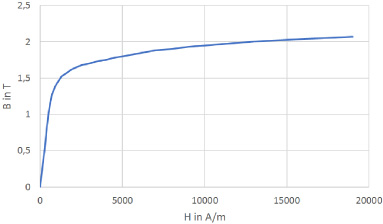
Fig. 1.

Nonlinear B–H curve in electromagnetism.

To solve the nonlinear PDE in ((3)), an operator

(7)

F(A)=0

is introduced. Following the approximation in [23], a linearization of ((7)) results in

(8)

F≈F(Ak)+F′(AK)[S]

with A_k+1 = A_k + S. Therein, the term F^′(A_K)[S] denotes the Frechét derivative of F at A_k in the direction of S and is used as discussed in [24] and [25]. The linearized form of the Frechét derivative results in

(9)

F′(AK)[S]≈F(Ak+S)−F(Ak).

Based on [23] and [26], the weak form of the PDE in ((3)) reads as follows: Find A ∈ H₀(curl) with the Sobolev space

(10)

H0(curl)={ψ∈(L2(Ω)3)∣∇×ψ∈(L2(Ω)3),n×ψ=0 on Γ}

such that

(11)

∫Ων(|∇×A|)(∇×A)⋅(∇×A′)dΩ=∫ΩJi⋅A′dΩ

for all test functions A^′ ∈ H₀(curl). There, 𝛺 considers a domain with boundary 𝛤. Subsequently, we arrive at fixed point method by

(12)

K(A_k)S_=f_−K(A_k)A_k.

Here, K is the global stiffness matrix depending on the magnetic vector potential A_k in the k-th iteration, S is the vector of unknowns, and f is the right hand side vector. A detailed derivation can be found in [23] and [27]. The updating procedure for the magnetic vector potential is performed by

(13)

A_k+1=A_k+ηS_.

The variable 𝜂 in ((13)) takes care for a non monotonic material relation and controls the convergence during the early steps of iteration. To determine the optimal relaxation parameter 𝜂, a line search method as explained in [28] is used.

Fig. 2.

Pole force evoked due to a permeability change with 𝜇₁ > 𝜇₂.

Pole force evoked due to a permeability change with 𝜇1 > 𝜇2.

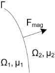
The physical quantity to optimize in this approach is the electromagnetic force at an interface as shown in Fig. 2, which is evoked by a permeability change. There are different approaches to compute the pole force as explained in [29] and [30]. We are following the ideas in [31] and [32] to compute the force by the use of Maxwell’s stress tensor. In [22], the Maxwell stress tensor is defined by

(14)

[fσ,mag]=H⊗B−12(BH)I.

Therein, I stands for the identity matrix. The surface force density is obtained by

(15)

fσ,mag=H(B⋅n)−12(B⋅H)n,

with the normal vector n. Finally, the pole force acting on the surface can be computed by

(16)

Fmag=∫V∇⋅[fσ,mag]dV=∮Sfσ,magdΓ.

The force computation by the use of Maxwell stress tensor requires a high mesh quality around the objects of interest as discussed in [33]. This is associated with a fine mesh discretization at the interface. A structured mesh with a high discretization rate results in an increase of computational effort due to the major amount of unknowns. The use of an unstructured mesh leads to numerical errors caused by distorted elements. This is why non-conforming interfaces as shown in [23] are introduced. Therein, Nitsche-type mortaring is based on the idea of discontinuous Galerking finite element methods at the interface as shown in [21] and [34]. The algebraic system results in

(17)

KA_+KΓA_=f_.

Therein, K_𝛤 is a symmetric coupling matrix. Further information is provided in [21] and [23].

3.Nodal and edge based finite element formulation

In electromagnetism, it is important to model the interface conditions between two media with different material properties in a correct physical manner. Thereby, the magnetic vector potential has to fulfill the following transmission conditions

(18)

A×n=0andn×ν∇×A=0.

A detailed derivation is given in [35]. In the 2D case, nodal elements are sufficient, because the interface conditions are fulfilled. In the 3D case, we have to use an edge based finite element formulation. Further information can be found in [36] and [37].

4.Topology optimization using the SIMP approach

Element wise design parametrization – or, as it is usually called, the SIMP approach – allows to formulate a material distribution problem of the type first discretize, then optimize. Based on the finite element discretization, we use element wise design variables 𝜌_e with the property

ρe={1for solid material and0for air,

forming the vector 𝜌 of design elements. The efficiency and success of the SIMP approach in solving design problems with a high number of design variables comes from the applicability of gradient based optimizers. For this purpose, differentiability is obtained by relaxing the parametrization to continuous variables 0 ≤ 𝜌_e ≤ 1. The design variable is introduced in [12] via the magnetic permeability. The approach in [13] and [6] shows, that sensitivity analysis is more stable by introducing the magnetic reluctivity 𝜈 as

(19)

ν(ρe)=ν0(1+(νr−1)ρe),

with the magnetic reluctivity in vacuum 𝜈₀ and the material dependent magnetic reluctivity 𝜈_r. Elements with a design variable 𝜌_e≠ 0 or 𝜌_e≠ 1 are called gray scale elements. Their material state is physically undefined. In the classical application of the SIMP approach (elastic stiffness maximization), the design variable is subject to an interpolation, typically power law, and some form of regularization, typically filtering. Hence a physical design variable ρepenal=H(ρe)p with filter function H and a so called penalization parameter p is used [10]. A filter technique is in the present case not required. Compared to [12], the problem is penalized with p = 1. A general discussion of this topic is provided in [38].

The parametrization leads to design dependent element stiffness matrices Ke(ρe). The design dependent global system matrix K(𝜌) has to be recomputed at each iteration of the optimization problem. For this, the converged stiffness matrix from the nonlinear PDE in ((12)) is used for assembling.

5.Sensitivity analysis by using the adjoint method

Our motivation is to maximize the attractive force F_mag in ((16)), typically acting on a specified interface. Equivalently, we may maximize the magnetic flux density B within a specified region. Any objective function to be optimized needs to provide a scalar value. We introduce the field function

(20)

JB(x)=⟨B(x),D(x)B(x)⟩.

Therein, a selection matrix D∈Rdim×dim allows to select a desired direction of the magnetic flux density as discussed in [14] and [15]. In the discrete finite element setting, ((20)) can be rewritten as

(21)

JBe=∑i=1Nip⁡A_e(Be,i⊤De Be,i)A_e.

In ((21)) JBe is the field function for element e, A_e is the element solution vector for the magnetic vector potential, Be is the element wise curl operator to be evaluated at all N_ip quadrature points, and D the selection matrix on element level. This follows the standard approach for setting up the finite element system, see [39] for more details.

The optimal design with respect to maximum force F_mag would be

(22)

JBint=∮AJB(x) dx,

in which x is the location, or in discrete form

(23)

JBsum=∑e=1NA⁡∑i=1Nip⁡A_e(Be,i⊤De Be,i)A_e,

with the set of chosen elements N_A. We can formally write ((23)) also in terms of the global finite element system as

(24)

JBglob=⟨B_A_,D_ B_A_⟩.

The optimization problem to maximize the magnetic force via the magnetic flux density can now be stated as

(25)

max ⟨B_A_,D_ B_A_⟩subject to K(ρ_)A_=f_,ρe∈[0;1], ∀e∈NΩ.}

In this approach we add a resource constraint for all design variables within the set of element indices N_𝛺.

In [12] the sensitivities are obtained from the continuum based equilibrium. In this approach we use the discretized equilibrium. The equivalent augmented cost function reads as

(26)

ΦB=⟨B_A_,D_ B_A_⟩+λ_⊤(K(ρ_)A_−f_).

Deriving ((26)) with respect to the design variable and sorting the state dependent terms results in

(27)

dΦBdρe=(2 A_⊤(B_⊤D_B_)+λ_⊤K(ρ_))∂A_∂ρe+λ_⊤∂K(ρ_)∂ρeA_.

The expression ∂A_∂ρe in ((27)) is expensive to compute. Hence, we choose 𝜆 such that the first term in ((27)) becomes zero, which is obtained when 𝜆 solves

(28)

K(ρ_) λ_=−2 (B_⊤D_ B_)A_.

Therein, we make use of a symmetric system matrix K(𝜌). To compute the adjoint system ((28)), we use the converged system matrix K. Using a direct solver, based on LU decomposition, the solution of the additional adjoint system comes by a minor cost. Since 𝜆 solves ((28)), the objective function in ((27)) computes as

(29)

dΦBsumdρe=λ_⊤∂K(ρ_)∂ρeA_.

For numerical efficiency, ((28)) can be implemented on element properties, similar to ((23)). As ∂K(ρ_)∂ρe has only contributions from a single element, ((29)) can be efficiently implemented as

(30)

dΦBsumdρe=λ_e⊤∂Ke(ρ_)∂ρeA_e.

The procedure is repeated until the convergence criterion is fulfilled. Density based topology optimization problems come with a large number of design variables and a first order sensitivity information which asks for a special class of optimizers. We have best results using SNOPT [40] and the Method of Moving Asymptotes (MMA) based SCPIP [41]. Alternatively the open source code IPOPT [42] may be used. The workflow of the optimization procedure is shown in Fig. 3 and is implemented in the finite element software CFS++ [43].

Fig. 3.

Optimization workflow for a topology optimization using SIMP method.

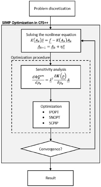
Fig. 4.

2D reference configuration for optimization.

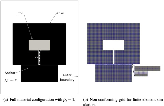
Fig. 5.

Optimization of the electromagnetic actuator from Fig. 4(a). An initial design variable was assumed by 𝜌_e = 0.4. The air gap distance between yoke and anchor was 1 mm. Additionally, a nonlinear material behaviour was assumed for yoke and anchor.

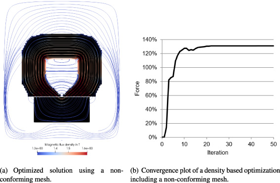
Fig. 6.

Comparison of the magnetic leakage flux for the nonlinear case in the air gap between the poles of the yoke along the dashed line from Fig. 4(a) between reference configuration (see Fig. 4(a)) and optimized design (see Fig. 5(a)). Here, the variable 𝛿 represents the range from the coil towards the anchor.

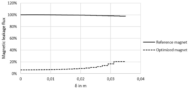
Fig. 7.

Optimized solution using non-conforming meshes in the air gap. The air gap distance between yoke and anchor is varied. A nonlinear material behaviour for anchor and yoke was taken into account.

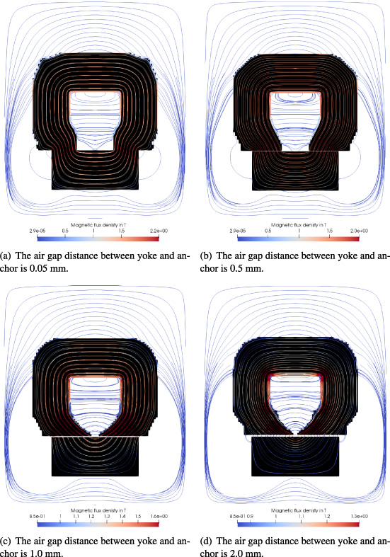
Fig. 8.

Force behaviour during iteration for different air gaps. The values were standardized to the maximum force value of each curve.

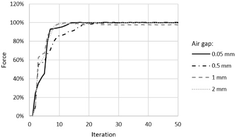
Fig. 9.

3D reference configuration for optimization.

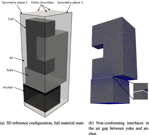
Fig. 10.

Convergence plot of a density based optimization. The reference configuration (full material) is shown in Fig. 9(a). The optimization starts with 𝜌_e = 0.4. Non-conform interfaces are used in the air gap. The air gap distance between yoke and anchor is 1 mm. Additionally, a nonlinear material behaviour is assumed for yoke and anchor.

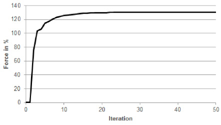
Fig. 11.

Optimized 3D geometry, assuming a nonlinear material behaviour for yoke and anchor. Interface conditions are fulfilled by the use of edge elements. Non-conforming interfaces are used in the air gap between yoke and anchor. The air gap distance between yoke and anchor is 1 mm.

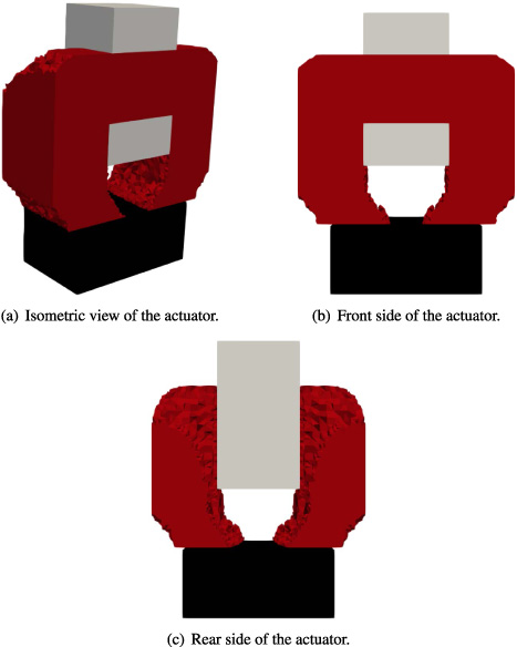
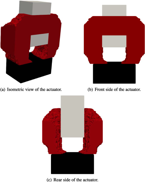
Fig. 12.

Optimized 3D geometry, assuming a linear material behaviour for yoke and anchor. Interface conditions are fulfilled by the use of edge elements. Non-conforming interfaces are used in the air gap between yoke and anchor. The air gap distance between yoke and anchor is 1 mm.

6.Numerical results

The electromagnetic actuator in 2D which has to be optimized is displayed in Fig. 4(a). It consists of a yoke, an anchor and a copper coil. A nonlinear material behaviour is assumed for the yoke and the anchor. Applying non-conforming interfaces based on Nitsche-type mortaring, we arrive at a non-conform mesh as shown in Fig. 4(b). The discretized configuration is optimized by a density based optimization approach. The copper coil is impressed by a current density

(31)

Ji=INcΓceJ.

Therein, I is the impressed current, N_c are the windings, 𝛤_c is the coil cross section and e_J is the vector pointing into the direction of the current. An electromagnetic field is generated in the yoke. The field lines between yoke and anchor are closed via an air gap. Furthermore, a nonlinear material behaviour was assumed for yoke and anchor. For discretization quadrilaterals with nodal elements of first order were used. Furthermore, the outer boundary of the surrounded air domain has to fulfill the condition

(32)

B⋅n=0→A×n=0,

with n defined as the normal vector. Our goal is to increase the magnetic force between anchor and yoke by optimizing the yoke domain. Besides, SNOPT from [40] was used as optimizer. The air gap distance between yoke and anchor was assumed with 1 mm. The finite element simulation was performed with a non-conform grid as shown in Fig. 4(b). Figure 5(a) shows the optimized result by the use of a non-conform mesh. The magnetic flux density is uniformly distributed over the cross section of the geometry. In contrast to the nonlinear solution presented in [12], the obtained result does not show any holes in the optimized topology. The convergence behaviour of the force is plotted in Fig. 5(b).

Obviously, a leakage flux between the two poles of the yoke (crossing the dashed line in Fig. 4(a)) can be minimized by expanding the gap between the two poles of the yoke as shown in Fig. 6. Therein, the magnetic leakage flux is plotted along the dashed line from Fig. 4(a). The variable 𝛿 in Fig. 6 represents the range from the coil towards the anchor as shown in Fig. 4(a). A further material reduction is performed in the upper and lower corners of the actuator as Fig. 5(a) shows. Moreover, the optimization results depend on the air gap distance between yoke and anchor as shown in Fig. 7. Therein, the air gap between yoke and anchor was varied in the range of 0.05 mm until 2 mm. Moreover, the initial design variable was chosen with 𝜌_e = 0.4 to obtain results under equal conditions. The results show a difference in the magnetic field distribution as well as in the optimized actuator design, especially at the poles of the yoke. The optimization was performed with a nonlinear material behaviour. Figure 8 shows the convergence of the force during optimization. For comparison, the values were standardized to the maximum force value of each curve. At the beginning of the optimization process there were differences in the convergence behavior. These disappear with an increasing number of iterations. Nevertheless, minor deviations occur due to the different material saturation states.

A 3D model of an electromagnetic actuator is shown in Fig. 9(a). It consists of a yoke and an anchor with nonlinear material behaviour. The impressed current density follows Eq. (31). On the outer boundary, (32) has to be fulfilled. Edge elements are used to fulfill the interface conditions. The non-conforming mesh in the air gap is shown in Fig. 9(b). Because of the major computational effort in 3D, symmetry conditions are used for symmetry plane 1 and 2 as shown in Fig. 9(a). A constant air gap between yoke and anchor of 1 mm was assumed.

The convergence behaviour is plotted in Fig. 10. Therein, a nonlinear material behaviour for the yoke and anchor was assumed. The optimization procedure starts with an initial design variable of 𝜌_e = 0.4. The obtained result is presented in Fig. 11(a). Figure 11(b) shows the optimized geometry from the front, and Fig. 11(c) from the rear side. Equally to the 2D example, a material reduction took place in the upper and lower corners of the yoke. The same applies to the poles of the yoke. Especially on the rear side of the yoke a major material reduction was performed. For comparison, optimization was also carried out under the assumption of a linear material behavior. The final result is presented in Fig. 12. A mentionable difference occurs at the poles of the yoke. This can be attributed to the increased magnetic flux concentration in the finite elements under the assumption of a linear magnetic material behaviour.

7.Conclusion and outlook

We showed a pseudo density topology optimization approach for the maximization of the magnetic force in the magnetostatic setting based on nonlinear material modeling, which is applicable in 3D. Additionally, non-conforming interfaces were introduced to prevent numerical errors due to distorted elements. Moreover, the number of unknowns reduces strongly.

The formulation of the objective function allows to maximize the magnetic flux density for a prescribed direction, and thus the magnetic force in a selected region. The pseudo density topology optimization parametrization (also known as SIMP¹ model) is used in combination with the adjoint approach. The sensitivity was derived from the discrete equilibrium. The design variables interpolate via the magnetic reluctivity between air and iron. An increase in penalization on the design variables was not necessary to obtain a clear distinct result. The optimization was performed without a volume constraint. By this, the obtained designs are of optimal shape with optimal volume fraction. In 3D edge elements are applied to fulfill the interface conditions. Besides, non-confoming interfaces are used to prevent numerical errors due to distorted elements. By this, the obtained designs are of optimal shape with optimal volume fraction. The gap between the poles in the optimized designs is such that the leakage flux is significantly below the flux of the initial configuration. Furthermore, the sharp corners of the yoke have been removed and results in a weight reduction.

References

[1]	O. Özkaraca, A review on usage of optimization methods in geothermal power generation, Mugla Journal of Science and Technology 4: (1) ((2018) ), 130–136.
[2]	R. Haupt, Comparison between genetic and gradient-based optimization algorithms for solving electromagnetics problems, IEEE Trans. Magn. 31: ((1995) ), 1932–1935.
[3]	C. Lalau-Keraly, S. Bhargava, O. Miller and E. Yablonovitch, Adjoint shape optimization applied to electromagnetic design, Optics Express 21: (18) ((2013) ), 21693–21701.
[4]	J. Haslinger and R. Mäkinen, Introduction to Shape Optimization - Theory, Approximation, and Computation, SIAM, (2003) .
[5]	A.A. Novotny and J. Sokolowski, Topological Derivatives in Shape Optimization, Springer, (2013) .
[6]	J. Byun and S. yop Hahn, Topology optimization of electrical devices using mutual energy and sensitivity, IEEE Trans Magn. 35: (5) ((1999) ), 3718–3720.
[7]	S. Sanogo and F. Messine, Topology optimization in electromagnetism using SIMP method: Issues of material interpolation schemes, COMPEL - The International Journal for Computation and Mathematics in Electrical and Electronic Engineering 37: (6) ((2018) ), 2138–2157.
[8]	M. Bendsøe, Optimal shape design as a material distribution problem, Struct. Multidisc. Optim. 1: ((1989) ), 193–202.
[9]	D. Dyck and D. Lowther, Automated design of magnetic devices by optimizing material distribution, IEEE Trans. Magn. 32: ((1996) ), 1188–1193.
[10]	M. Bendsøe and O. Sigmund, Topology Optimization Theory, Methods and Applications, Springer, (2009) .
[11]	R. Youness and F. Messine, An implementation of adjoint based topology optimization in magnetostatics, COMPEL - The International Journal for Computation and Mathematics in Electrical and Electronic Engineering 38: (3) ((2019) ), 1023–1035.
[12]	S. Wang and J. Kang, Topology optimization of nonlinear magnetostatics, IEEE Trans. Magn. 38: (2) ((2002) ), 1029–1032.
[13]	J.S. Choi and J. Yoo, Structural optimization of ferromagnetic materials based on the magnetic reluctivity for magnetic field problems, Comput. Meth. Appl. Mech. Engrg 197: ((2008) ), 4193–4206.
[14]	S. Wang, D. Youn, H. Moon and J. Kang, Topology optimization of electromagnetic systems considering magnetization direction, IEEE Trans. Magn. 41: (5) ((2005) ), 1808–1811.
[15]	J. Yoo, S. Yang and J.S. Choi, Optimal design of an electromagnetic coupler to maximize force to a specific direction, IEEE Trans. Magn. 44: (7) ((2008) ), 1737–1742.
[16]	P. Seebacher, M. Kaltenbacher, F. Wein and H. Lehmann, Optimization of an electromagnetic actuator using topology-optimization, COMPUMAG ((2019) ).
[17]	M. Bendsøe and O. Sigmund, Material interpolation schemes in topology optimization, Arch. Appl. Mech. 69: ((1999) ), 635–654.
[18]	T. Labbé and B. Dehez, Convexity-oriented mapping method for the topology optimization of electromagnetic devices composed of iron and coils, IEEE Trans. Magn. 46: (5) ((2010) ), 1177–1185.
[19]	J.S. Choi and J. Yoo, Simultaneous structural topology optimization of electromagnetic sources and ferromagnetic materials, Comput. Meth. Appl. Mech. Engrg 198: ((2009) ), 2111–2121.
[20]	J. Lee, J. Kook and S. Wang, Multi-domain topology optimization of pulsed magnetic field generator sourced by harmonic current excitation, IEEE Trans. Magn. 48: (2) ((2012) ), 475–478.
[21]	K. Roppert, F. Toth and M. Kaltenbacher, Modelling nonlinear steady state induction heating processes, IEEE Trans. Magn. 56: (3) ((2020) ), 287–290.
[22]	J. Stratton, Electromagnetic Theory, IEEE Press, (2007) .
[23]	M. Kaltenbacher, Numerical Simulation of Mechatronic Sensors and Actuators, Springer, (2015) .
[24]	D. Behmardi and E. Nayeri, Introduction of Frechét and Gâteaux Derivative, Appl. Math. Sci. 2: (20) ((2008) ), 975–980.
[25]	M.C. Delfour and G. Sabidussi, Shape optimization and free boundaries, NATO Adv. Sci. Inst. Ser. M 380: ((1990) ).
[26]	C. Song and Z. Qun, Multiphysics Modeling - Numerical Methods and Engineering Applications, Academic Press, Elsevier, (2016) .
[27]	J. Nocedal and S.J. Wright, Numerical Optimization, Springer, (1987) .
[28]	O. Zienkiewicz, R. Taylor and P. Nithiarasu, The Finite Element Method, Vol. 6, Elsevier/Butterworth-Heinemann, Oxford, (2005) .
[29]	J. Coulomb and G. Meunier, Finite element implementation of virtual work principle for magnetic or electric force and torque computation, IEEE Trans. Magn. 20: ((1984) ), 1894–1896.
[30]	F. Henrotte and K. Hameyer, Computation of electromagnetic force densities: Maxwell stress tensor vs. virtual work principle, J. Comput. Appl. Math. 168: ((2004) ), 235–243.
[31]	Z. Ren and A. Razek, Force calculation by Maxwell stress-tensor in 3D hybrid finite element-boundary integral formulation, IEEE Trans Magn. 26: (5) ((1990) ), 2774–2776.
[32]	M.K. Ghosh, Y. Gao, H. Dozono, K. Muramatsu, W. Guan and J. Yuan, Proposal of Maxwell stress tensor for local force calculation in magnetic body, IEEE Trans. Magn. 54: ((2018) ).
[33]	S. Ho, S. Niu, W. Fu and J. Zhu, A mesh-intensive methodology for magnetic force computation in finite-element analysis, IEEE Trans. Magn. 48: (2) ((2012) ), 287–290.
[34]	A. Hansbo and P. Hansbo, An unfitted finite element method, based on Nitsches method for elliptic interface problems, Comput. Meth. Appl. Mech. Engrg 191: ((2002) ), 5537–5552.
[35]	M.N.O. Sadiku, Numerical Techniques in Electromagnetics, CRC Press, (2000) .
[36]	G. Mur, Edge elements, their advantages and their disadvantages, IEEE Trans. Magn. 30: (5) ((1994) ), 3552–3557.
[37]	J. Nédélec, Mixed finite element in 3D in H(div) and H(curl), Proc. Intl Conf. Differ. Equ. Appl. 1192: ((1986) ), 321–325.
[38]	F. Wein, M. Kaltenbacher, B. Kaltenbacher, G. Leugering, E. Bänsch and F. Schury, On the effect of self-penalization of piezoelectric composites in topology optimization, Struct. Multidisc. Optim. 43: (3) ((2011) ), 405–417.
[39]	A. Kost, Numerische Methoden in der Berechnung Elektromagnetischer Felder, Springer, (1994) .
[40]	P. Gill, W. Murray and M. Saunders, SNOPT: An SQP algorithm for large-scale constrained optimization, SIAM J. Optim. 12: (4) ((2005) ), 979–1006.
[41]	C. Zillober, SCPIP – an efficient software tool for the solution of structural optimization problems, Struct. Multidisc. Optim. 24: ((2002) ), 362–371.
[42]	A. Waechter and L. Biegler, On the implementation of an interior-point filter line-search algorithm for large-scale nonlinear programming, Math. Program. Ser. A 106: ((2005) ), 25–57.
[43]	M. Kaltenbacher, Advanced simulation tool for the design of sensors and actuators, in: Procedia Engineering, Proc. Eurosensors XXIV, Linz, Austria, Vol. 5, (2010) , pp. 597–600.

Notes

1 Solid Isotropic Material with Penalization