A computational framework for finding parameter sets associated with chaotic dynamics

1Introduction

Chaos is known to occur in many natural biological systems involving population dynamics [10, 12, 13, 17]. For example, Becks et al. demonstrated existence of chaotic and non-chaotic states in an experimental study of a microbial predator-prey system with a nutrient source [7]. The authors used daily measurements of the population size of each species to document transitions between chaotic and non-chaotic states after changing the strength of the nutrient source. Another experimental study involving baker’s yeast and a fermenter [11] also observed chaotic fluctuations in the growth rate of the fungus. The paper demonstrated chaotic behavior through time series analysis.

Even simple dynamical system models are known to exhibit chaotic behavior for certain values of system parameters [19, 28]. However, even such simple systems can possess a wide range of chaotic and non-chaotic behavior, related in a non-trivial way to certain combinations of system parameters and initial conditions. As a result, detecting and analyzing chaotic behavior is far from straightforward and requires a high degree of mathematical sophistication. This can pose a significant challenge to modelers with a mostly biological background and hinder the discussion of chaotic dynamics in biological systems for educational purposes.

In this work, we evaluate the ability of standard computational tools to find subsets of the parameter space which give rise to positive Lyapunov exponents. In particular, we use optimization algorithms to efficiently search the parameter space and return values which define arrangements of dynamical systems giving computationally positive Lyapunov exponents. The framework uses numerical techniques to generate approximate solutions to the dynamical system coupled with optimization algorithms to uncover connections between parameters and highlight regions of chaos.

We pair the results from the optimization with visualization tools available in R to allow investigators to easily establish relationships between parameter choices and identify ranges of parameter values leading to chaotic behavior. The aim is to help biologists develop a better understanding of the causes of chaotic behavior in dynamical systems without having to master the intricate mathematical analysis often required to rigorously detect and analyze chaotic behavior. The main novelty of the approach is the use of optimization algorithms and high-dimensional visualization techniques to assist with identification and understanding of parameters leading to chaotic dynamics.

We validate our computational approach by applying it to population models in the literature. The equations in the systems we considered contain rate-limited functions to model predator/prey dynamics. Systems of this type have been well studied in chemostat environments, both experimentally and analytically [3, 7, 17, 19]. They have been shown to demonstrate chaotic dynamics [7, 6, 14] and can be considered as small-scale studies for larger ecological systems [4]. In particular, we consider the set of coupled differential equations

Given the wide applicability of these models to different physical and ecological systems, we seek to better understand the choices of model parameters and initial conditions leading to chaotic behavior. Let P ⊆ R^m denote all possible valid settings for the m parameters in our system (e.g., one parameter might describe the dilution rate which is the rate at which a nutrient is introduced into the system). Let I ⊆ Rⁿ denote the set of all valid initial conditions for (Y₁, Y₂, …, Y_n). Defining S = P × I, we seek to characterize the regions of S leading to chaotic behavior. A particular region s ∈ S is deemed chaotic if it has negative divergence at its initial conditions (to ensure boundedness) and yields a positive Lyapunov exponent. In our computations we use standard numerical integrators for ordinary differential equations along with popular methods for numerical Lyapunov exponent calculation [8, 31].

In the following sections, we describe the algorithms and visualizations used in our approach, we provide the results from the validation exercises, and we summarize our findings and provide discussion on future research directions.

2Description of the framework

The framework discussed in this paper uses the freely available software tools COPASI (a COmplex PAthway SImulator) [16] and R [26] to compute the Lyapunov exponents, evaluate the objective functions, and construct parallel coordinates visualizations of the results. The flowchart in Fig. 1 shows the progression of the algorithm.

Fig. 1

Flowchart of the simulation framework. The data returned from COPASI is handed to R to generate the parallel coordinates visualization. Any optimization algorithm can be used to explore the design space.

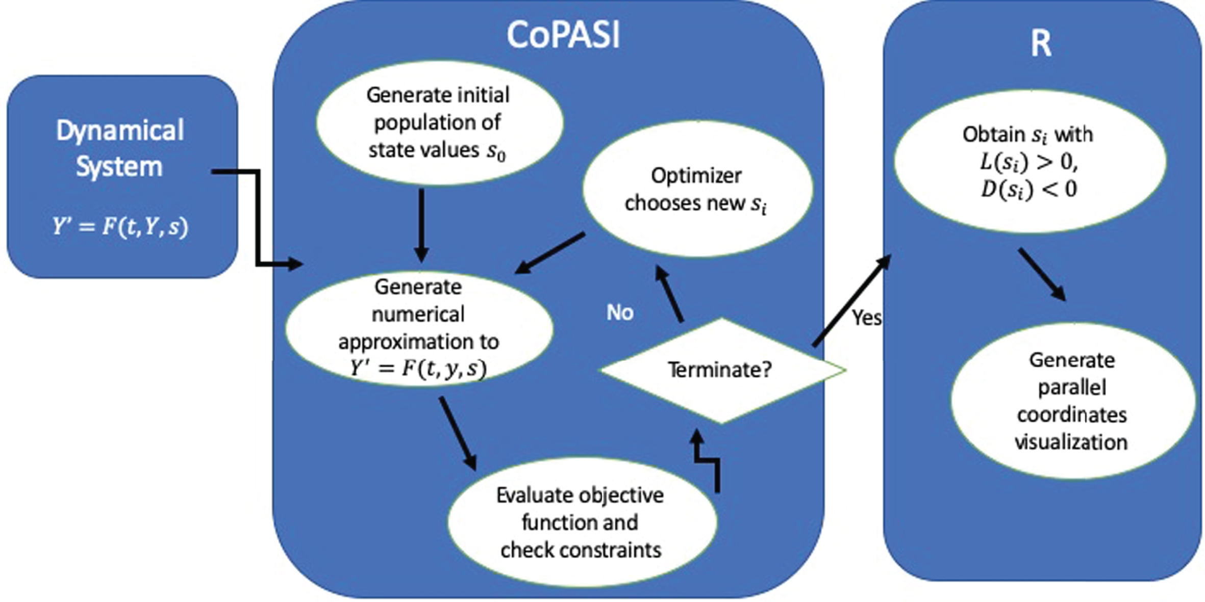
Let Y′ = f (t, Y, s) represent a dynamical system with parameters s ∈ S. If the system models population dynamics, for instance, the parameters can contain birth and death rates along with initial conditions. We take S to be the design space in this framework.

The usual test for chaos is calculation of the largest Lyapunov exponent; a positive largest Lyapunov exponent indicates chaos [29]. Lyapunov exponents provide a quantitative measure of the convergence or divergence of nearby trajectories for a dynamical system. The system is said to be chaotic over s ∈ S if the maximum Lyapunov exponent L (s) is positive and the diverence of the system D (s) is negative [2]. The divergence of the system is defined as the trace of the Jacobian associated with the system evaluated at the initial state. That is, the system exhibits chaotic dynamics if L (s) >0 and D (s) <0. Thus, our overall objective is to efficiently search S to find members s in the space for which the maximum Lyapunov exponent L (s) >0 and for which the divergence D (s) <0.

Strategies for computing the Lyapunov spectrum for a dynamical system have been known for some time [31]. At the heart of these algorithms is an efficient computational technique for generating accurate numerical approximations to the system. Our interest is in the inverse problem; that is, given a dynamical system with an associated parameter space, is it possible to use numerical tools to find elements in the space which result in a positive Lyapunov exponent for the system? In addition, we wanted to gain insight into the possible connections between the parameter values leading to these positive exponents. Thus, we used visualization tools to generate graphical representations of these associations.

The algorithm in Wolf, et al. [31] actually computes the entire Lyapunov spectrum from the discretized solution to the system of ordinary differential equations (ODEs) and the associated linearized equations of motion. The linearized equations of motion are formed from the Jacobian of the system of ordinary differential equations. We use the implementation of this algorithm available in COPASI.

The objective function defined for the optimization routine is to maximize the maximum Lyapunov exponent for a given dynamical system Y′ = f (t, Y, s), over a paramter set s. That is, starting with the definition of the dynamical system and the initial parameter set s₀, the optimization algorithm computes the maximum Lyapunov exponent and the divergence of the system associated with that particular parameter set. The optimization problem is constrained by the divergence. That is, the Lyapunov exponent must be positive, and the divergence negative, for this parameter set to be feasible. We note most optimization algorithms minimize objective functions, so our objective function is actually the negative of the maximum Lyapunov exponent.

Based on the information returned from the evaluation of the objective function, the optimization routine then chooses another parameter set s₁ and again computes the maximum Lyapunov exponent and divergence for that parameter set. This process continues until the optimization algorithm exhausts its set of function evaluations or determines progress is no longer being made in maximizing (or minimizing) the objective.

We chose to use the genetic algorithm available in COPASI [16] as the optimization algorithm. Genetic algorithms move through “generations" of design points by evaluating the fitness of members of the generation and selecting members to continue to the next generation (through mutation or cloning), parent offspring for the next generation, or die (i.e., these points are removed from the population) [24]. The algorithm was run multiple times, with different initial choices for parameters, to look for multiple design points.

These results were validated with the simulated annealing optimization routine also available in COPASI. The simulated annealing algorithm randomly selects design points and keeps those which are associated with lower objective function evaluations. In order to make the search global, the algorithm also selects a few random points which increase the value of the objective function. The algorithm moves to a new state or remains in a given state with a specified probability, with an increased probability associated with those states giving lower values of the objective function. The behavior of the algorithm is defined by choosing parameters which define the size of the initial search region and reduce the size of the search space as the algorithm progresses [1, 9].

Let C ⊆ S denote the subset of all parameters and initial conditions leading to chaotic behavior. Now that we have a method for efficiently generating samples from the chaotic regime C, we use an interactive visualization platform to help the user understand the structure of C —a challenging task, due to the potentially complex, high-dimensional nature of this set. Our platform is based on parallel coordinates, a popular means of visualizing high-dimensional data. The plots were generated using the plotly [27] package in R. The input for the parallel coordinates was obtained from the result files from the optimization task of COPASI. All COPASI and R files can be found in https://github.com/skoshyc/Computational-Framework-Chaotic-Dynamics.

Figure 2 shows an example of sample points with a positive Lyapunov exponent generated from the equations of the well-known Lorenz system [22]. The set of ODE equations in [22] is given as

Parallel coordinate plots allow us to understand a number of useful properties by visual inspection and interactive manipulation. For example, in Fig. 2, we see that chaos can be obtained for log (r) ∈ (4.55, 4.6) and values of b ∈ (2.60, 2.63). The purple line depicts one particular combination of the parameters and the Lyapunov exponent. The faint lines are combinations outside the selected range of log (r). By restricting several coordinates at a time, the user can filter an initially large number of sample points down to only a few.

Fig. 2

Chaotic samples visualized using parallel coordinates and obtained using the Lorenz system [22]. Note the narrow range of values for log (r) and b. For the purpose of the example, only 50 runs of the genetic algorithm were run. The pink line in ln (r) axis represents the user-defined choice of parameter range. The faint grey lines depict parameters that fall outside the user-defined choice.

3Numerical results

The numerical results presented are intended to demonstrate the ability of the framework to meet the stated goal of this work; i.e., provide researchers with a convenient numerical tool for exploring the parameter space and uncovering regions where parameter choices lead to chaos. We validated the framework on several dynamical systems from the literature. We include results from two of those studies here [14, 19].

Both of the included systems can be used to model predator-prey dynamics in ecosystems. The mathematical analysis of both systems uncovered parameter values which gave chaotic solutions [14, 19]. We sought to replicate these findings by maximizing the Lyapunov exponent over a design space consisting of the initial conditions for the variables and two of the parameters used to define the ODEs. We use this section to describe the equations and the results of our study.

All computations were carried out on a Windows 10 PC with Intel(R) CPU and 4 Cores. The version of COPASI was 4.27 and R was 4.0.0. Both the genetic algorithm and simulated annealing were run multiple times to obtain multiple sample points. Each run had randomized start values which is an option in the optimization task in COPASI. After each run, the maximum Lyapunov exponent along with the optimal parameters are generated. COPASI collects the information from each run and provides the output from all the runs in a text file. The positive Lyapunov exponents and associated parameter set are chosen by R and visualized using the parallel coordinates plot.

We used 200 generations with 20 population members in each genetic algorithm search to generate the results provided below. The algorithm was run 100 times to generate the parallel coordinates plots. For the simulated annealing results, we used the COPASI default parameter values for the starting temperature, the cooling factor, and the tolerance [1]. The start temperature defines the size of the random perturbations on the parameters for the algorithm, and the cooling factor defines the size of the reduction of the random perturbations at each cycle. The algorithm stops when the change in the objective function has been smaller than the tolerance in the last two temperature steps. The simulated annealing algorithm was run 25 times in order to have a defined number of points to compare with the results from the genetic algorithm. The number of repeated runs was limited due to the computational expense of the simulated annealing algorithm.

3.1Double forced Monod system (DFMS)

We first consider one of the dynamical systems presented and analyzed in work by Kot, Sayler, and Schultz [19]. While experimental results are not included in the paper, the authors justify their choice to study this particular system by noting the possibility of obtaining experimental validation of their work. As our primary interest in developing the framework presented here is to aid biologists in their data-based studies of dynamical systems, this particular problem presents an ideal benchmark case.

The dimensionalized equations for the DFMS are given as

dSdt=D[Si(1+εsin(2πTt))-S]-μ1Y1SHK1+SdHdt=μ1SHK1+S-DH-μ2Y2HPK2+HdPdt=μ2HPK2+H-DP,

where S represents the limiting substrate, H represents a prey species, and P represents a predator species. We note the predator species consumes only the prey, so its population is indirectly associated with the changes in S. The parameters in the model govern the response of the organisms to changes in the system. D is the dilution rate, which defines the ratio of the flow into the chemostat to the volume of organisms in the chemostat; μ₁ and μ₂ are the maximum specific growth rates of the prey and predator, respectively; Y₁ is the yield of prey per unit mass of substrate, and Y₂ is the yield of predator per unit mass of prey; and K₁ and K₂ are the half-saturation constants.

S_i is the inflowing substrate concentration where i denotes inflow of the substrate into the chemostat. We note the parameter ε changes the dynamics of the inflowing substrate. Smaller values of ε lead to more constant inflows, while larger values of ε introduce more fluctuation into the inflow. Both ε and the frequency of the associated oscillation were important parameters for chaos, indicating nutrition rates play an important role here.

The equations are nondimensionalized by rescaling all variables by the inflow substrate, the prey by its yield constant Y₁, and the predator by both yield constants [19]. The dimensionless system is given by

dxdτ=1+εsin(ωτ)-x-Axya+xdydτ=Axya+x-y-Byzb+ydzdτ=Byzb+y-z,

where x=SSi , y=HY1Si , and z=PY1Y2Si , τ = Dt, and ω=2πDT . Also, A=μ1D , a=K1Si , B=μ2D , and b=K2Y1Si .

As shown in the referenced paper, the dimensionless system exhibits chaotic behavior for ω=5π6 and ε = 0.6, with S_i = 115 mg/l, D = 0.1 / h, and initial conditions x (0) =0.42, y (0) =0.4, z (0) =0.42. The remainder of the parameter values are provided in Table 1. Representative manifold plots are given in [19] and are not duplicated here.

Table 1

Parameter values associated with the chaotic system described in [19].

	Yi	μi (h- 1)	Ki (mg/l)
Prey (i = 1)	0.4	0.5	8
Predator (i = 2)	0.6	0.2	9

To determine if our framework could recover the values cited in [19], we used the optimization algorithms to maximize the computed Lyapunov exponent as a function of ε, ω, and the initial states for x (τ), y (τ), and z (τ). A subset of our results is shown using parallel coordinates visualization in Fig. 3. This visualization indicates more positive Lyapunov exponents associated with small values of ω. Note in the rescaled system ω is the angular frequency of the forcing term. Thus, observing positive Lyapunov exponents for small values of ω may indicate to a biologist an interesting connection between periodic forcing and chaotic behavior that they may be able to further study experimentally. Any clustering of the remainder of the parameters chosen for our study is less obvious. Figure 4 contains a manifold plot of the dimensionless system for a randomly chosen set of parameter values from those discovered by our framework; namely, ε = 0.753444, ω = 0.455121, and initial conditions x (0) =4.49844, y (0) =0.428112, and z (0) =0.446482. We note that the strange attractor shown in Fig. 4 is distinct from the one given in the referenced paper.

Fig. 3

Results from the parameter search for the double forced Monod system in [19] visualized using parallel coordinates. The vertical axes are associated with values for the maximum calculated Lyapunov exponent, ε, ω, x (0), y (0), and z (0). The results are from 100 runs of the genetic algorithm in COPASI. The pink line in ε axis represents the user-defined choice of parameter range. The faint grey lines depict parameters that fall outside the user-defined choice.

Fig. 4

Manifold plot of forced model in [19]. Note the strange attractor is distinct from the one given in the paper.

To further investigate the efficacy of having a targeted search of the parameter space, we also used the simulated annealing approach of COPASI to generate a comparison of Lyapunov exponents with the results of the genetic algorithm. The initial conditions were set to (x, y, z) = (1, 1, 1) to observe the behavior of only the two parameters ε and ω. Each of the algorithms were run 25 times for the comparison. The comparison was repeated twice to account for stochasticity. As is seen in Fig. 5, there are clusters of positive Lyapunov exponents (and hence chaos) in the ranges of ε ∈ (0.18, 0.21) and ω ∈ (0.8, 1).

Fig. 5

Comparison of results from simulated annealing and the genetic algorithm with the initial conditions as (1, 1, 1). The two figures 5A and 5B are from running the comparison search twice. In each search, the algorithms are run 25 times. The regions of positive Lyapunov exponents are the same in each figure.

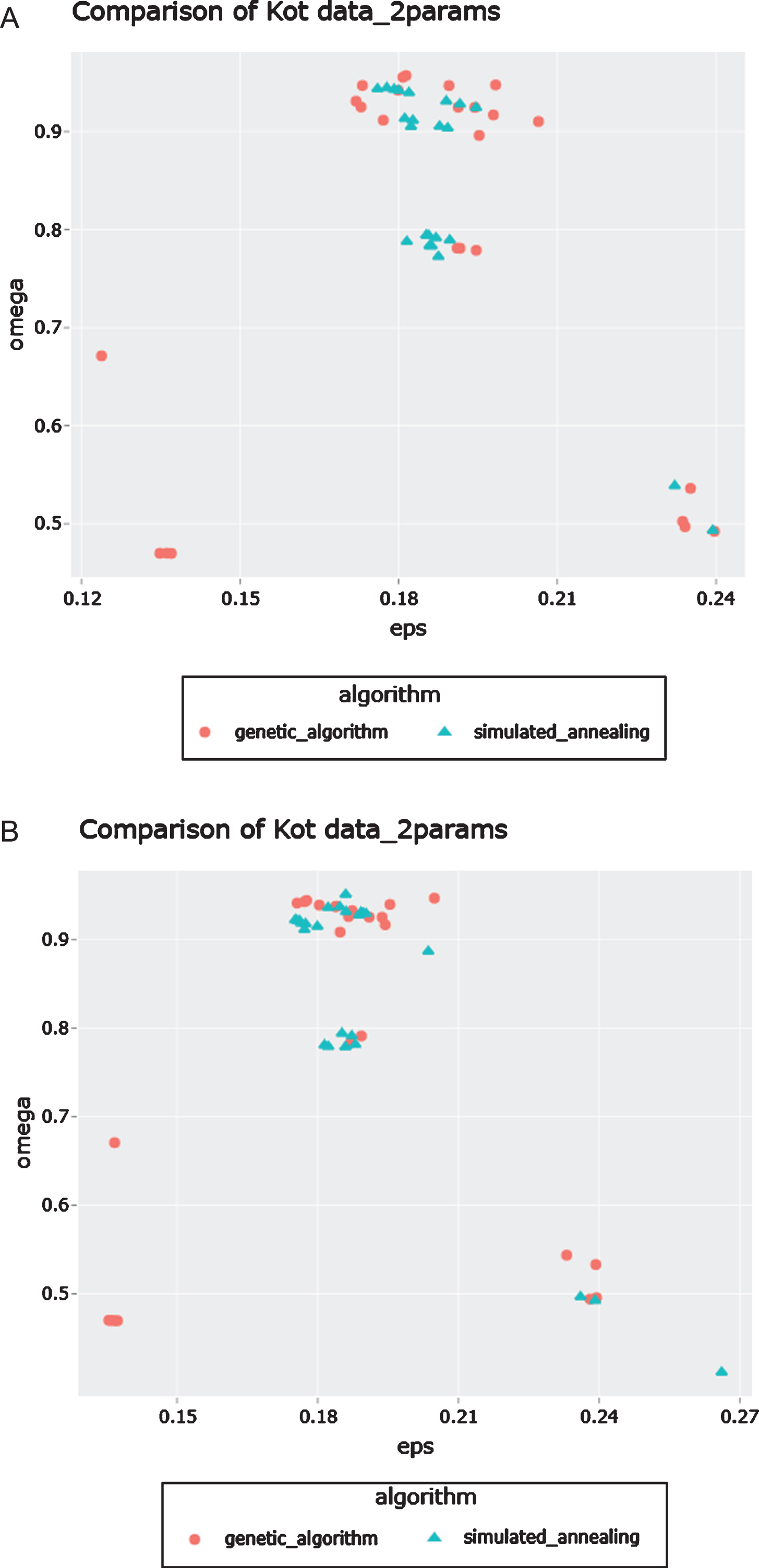
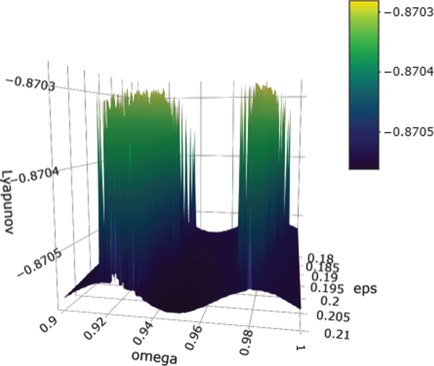
We sought to better understand these results by computing the maximum Lyapunov exponent over a 100 × 100 discretization of the region ε × ω for ε ∈ (0.18, 0.21), ω ∈ (0.9, 1) using the initial condition (1, 1, 1). The task was completed using the parameter scan option in COPASI. The results are shown in Fig. 6. The graph shows all of the largest Lyapunov exponents at these discrete points were negative, indicating the optimization algorithms were able to locate these small regions where positive Lyapunov exponents were computed. One of the reasons we possibly don’t get the requisite parameters in the 100 × 100 grid search is because the grid is regularly spaced. For example, two of the values associated with the cluster in Fig. 5 are (ε, ω) = (0.180791, 0.955417) , (0.181136, 0.913295). Such numbers do not appear in the regularly spaced grid search.

Fig. 6

Surface plot of Lyapunov exponents obtained for ε ∈ (0.18, 0.21) and ω ∈ (0.9, 1) with initial conditions (1, 1, 1).

3.2A three-species food chain

The second example uses a three-species food chain model where chaos was observed for a given set of biologically relevant parameters [14]. The model was a continuous, non-linear system which has biological implications of chaos on a general food web model. Our algorithm was able to find the same parameter values reported in the paper along with other parameter choices which lead to chaos.

This three-species model [14] is defined using the equations

dXdT=R0X(1-XK0)-C1F1(X)YdYdT=F1(X)Y-F2(Y)Z-D1YdZdT=C2F2(Y)Z-D2Z,

where

Fi(U)=AiUBi+Ui=1,2.

The variables X, Y, Z represent three species with X being the prey for Y and Y being the prey for Z. T represents time. The parameters are R₀, the intrinsic growth rate; K₀, the carrying capacity of species X; C₁ and C₂, the conversion rates of prey to predator for species Y and Z, respectively; and D₁ and D₂, the constant death rates for species Y and Z, respectively. The functions F_i (U) are a Monod type response to the prey species.

The authors created a nondimensional system of equations using the following transformations:

x=XK0y=C1YK0z=C1ZC2K0t=R0T.

The system used in our analysis is the nondimensional system given by

dxdt=x(1-x)-f1(x)ydydt=f1(x)y-f2(y)z-d1ydzdt=f2(y)z-d2z,

where f_i (u) = a_i (u)/(1 + b_iu)  i = 1, 2. The parameter values in the nondimensionalized system for which the authors of [14] observed chaos are in Table 2. The range of b₁ they studied was b₁ ∈ (2, 6). In addition, they observed chaotic dynamics for some values of b₂ which were not given in their paper.

Table 2

Parameter values associated with the chaotic system described in [14].

Parameters	Values
a1	5.0
b1	3.0
a2	0.1
b2	2.0
d1	0.4
d2	0.01

For our design space, we considered b₁ ∈ (2.5, 4), b₂ ∈ (1, 3), and ranges for the initial conditions x (0) ∈ (0.1, 1), y (0) ∈ (0.1, 1), and z (0) ∈ (7.5, 10.5).

The results obtained from this search are provided in Table 3 and Fig. 7. The authors of [14] note chaos is observed for larger values of b₂ (i.e. larger than 2), which we observe in the parallel coordinates plot as well. We also see that most of the positive Lyapunov exponents are found when b₁ and b₂ are both close to 2.5.

Table 3

Subset of the results from the genetic algorithm search for the three-species food chain in [14]

Lyapunov exponent	b1	b2	x (0)	y (0)	z (0)
0.023648	2.63651	2.59459	0.332151	0.220724	9.03868
0.0234837	2.5	2.45609	0.112289	0.292607	10.1235
0.0253758	2.51406	2.67227	0.143063	0.188911	10.5
0.0247539	2.52096	2.63509	0.170619	0.373552	10.5
0.0235603	2.57053	2.56936	0.165032	0.255972	10.5
0.0253312	2.5	2.64983	0.149159	0.199885	10.5
0.0290962	2.5	2.67319	0.28922	0.286104	9.83263
0.0227857	2.56591	2.65262	0.267509	0.255673	9.38101
0.0277303	2.6796	2.66453	0.1	0.289252	9.94014
0.0241472	2.5	2.64446	0.146135	0.112823	10.5

Fig. 7

Results from the parameter search for the three species food chain in [14] visualized using parallel coordinates. The vertical axes are associated with values for the maximum calculated Lyapunov exponent b₁, b₂, x (0), y (0), and z (0). The pink line in b₁ axis represents the user-defined choice of parameter range.

A comparison of simulated annealing and the genetic algorithm was performed to better understand the landscape of the Lyapunov exponents as a function of (b₁, b₂) with the initial conditions set to (0.5, 0.3, 9). As seen in Fig. 8, the majority of the parameter combinations which show chaos are centered around (b₁ = 2.5, b₂ = 2.5).

Fig. 8

Comparison of results from simulated annealing and the genetic algorithm search for chaos in the three species food chain in [14] with the initial conditions as (0.5, 0.3, 9).

4Conclusion

We have provided a computational strategy that allows researchers to efficiently search over a design space including parameter values and initial conditions and discover possible connections between values of these constants and chaotic dynamics. The ability for such a search may reveal chaotic behavior in systems not previously known to have chaotic regime and the existence of parameters and initial conditions not previously known to yield chaotic behavior in studied systems. In one of the models we investigated, our technique found chaotic regions which were not observed using a regularly spaced grid search. This showed that to obtain the chaotic parameters, we would need a finer grid and thus several more iterations. Another brute force technique such as a random search may also miss the chaotic parameters. The use of COPASI and R results in a robust, comprehensive framework for analyzing a given dynamical system without the need for rigorous mathematical analysis.

One of the main strengths of this approach is that it allows the study of system behavior that is virtually impossible to observe in a laboratory environment, thus making it useful to experimentalists. The parallel coordinates plots provide further insight into system dynamics for a wide variety of parameter changes.

Parallel computations will improve the efficiency of this strategy. The genetic algorithm is conceptually easy to parallelize, in that objective function evaluations for a generation can be easily distributed across processors. We have not evaluated the speed-up which would be associated with this modification. We also continue to evaluate the ability of different objective functions to locate parameter values associated with chaos. One of the Lyapunov exponents being positive is the chaos indicator that we employ in this paper. The optimization algorithm which searches for the maximal Lyapunov exponent will find the conditions which give the most positive exponent. As the Lyapunov exponent can be a discontinuous function of the design space, it can be easy for an optimization algorithm based on properties of continuous functions to miss them. Thus, better strategies for finding these points are warranted. If the system has two positive Lyapunov exponents, we are limited in the use of an optimization algorithm as the algorithm will probably give us the parameters which give rise to the more positive exponent thus missing other regions of chaos. However, multiple runs of global optimization algorithms like the genetic algorithm, simulated annealing, evolutionary algorithms in COPASI would give us different parameter combinations of the desired chaotic regions.

References

[1] | http://copasi.org/Support/User_Manual/Methods/Optimization_Methods/Simulated_Annealing/. [Last accessed: Jan 24, 2020]. |
[2] | Kathleen T. , Alligood T.S. and Yorke James A. , Chaos: an introduction to dynamical systems. Springer, (1997) . |
[3] | Banks H.T. , Modeling and Control in the Biomedical Sciences, volume 6 of Lecture Notes in Biomathematics. Springer-Verlag, Heidelberg, (1975) . |
[4] | Banks H.T. and Davidian M. , Introduction to the chemostat. http://www.ncsu.edu/crsc/htbanks/STMA810c/chemostat.pdf, 2009. |
[5] | Barrio R. and Serrano S. , A three-parametric study of the lorenz model, Physica D: Nonlinear Phenomena 229: (1) ((2007) ), 43–51. |
[6] | Becks L. and Arndt H. , Transitions from stable equilibria to chaos, and back, in an experimental food web, Ecology 89: ((2008) ), 3222–3226. |
[7] | Becks L. , Hilker F.M. , Malchow H. , Jürgens K. and Arndt H. , Experimental demonstration of chaos in a microbial food web, Nature 435: ((2005) ), 1226–1229. |
[8] | Benettin G. , Galgani L. , Giorgilli A. and Strelcyn J.-M. , Lyapunov characteristic exponents for smooth dynamical systems and for Hamiltonian systems: a method for computing all of them, Meccanica 15: (1) ((1980) ), 21–30. |
[9] | Corana A. , Marchesi M. , Martini C. and Ridella S. , Minimizing multimodal functions of continuous variables with the simulated annealing algorithm, ACM Trans Math Softw 13: ((1987) ), 262–280. |
[10] | Costantino R. , Desharnais R. , Cushing J. and Dennis B. , Chaotic dynamics in an insect population, Science 275: ((1997) ), 389–391. |
[11] | Davey Hazel M. , Davey Christopher L. , Woodward Andrew M. , Edmonds Andrew N. , Lee Alvin W. and Kell Douglas B. , Oscillatory, stochastic and chaotic growth rate uctuations in permittistatically controlled yeast cultures, Biosystems 39: (1) ((1996) ), 43–61. |
[12] | Dennis B. , Desharnais R. , Cushing J. and Costantino R. , Transitions in population dynamics: equilibria to periodic cycles to aperiodic cycles, J Anim Ecol 66: ((1997) ), 704–729. |
[13] | Fussmann G. , Ellner S. , Shertzer K. and Hairston N. , Crossing the Hopf bifurcation in a live predator-prey system, Science 290: ((2000) ), 1358–1360. |
[14] | Hastings A. and Powell T. , Chaos in a three-species food chain, Ecology 72: (3) ((1991) ), 896–903. |
[15] | Henson M.A. , Dynamic modeling of microbial cell populations, Curr Opin Biotech 14: ((2003) ), 460–467. |
[16] | Hoops S. , Sahle S. , Gauges R. , Lee C. , Pahle Jürgen , Simus N. , Singhal M. , Xu L. , Mendes P. and Kummer U. , Copasi|a complex pathway simulator, Bioinformatics 22: (24) ((2006) ), 3067–3074. |
[17] | Jost J. , Drake J. , Frederickson A. and Tsuchiya H. , Interactions of Tetrahymena pyrifarmis, Escherichia coli, Azobacter vinelndil, and glucose in a mineral medium, J Bacteriol 113: ((1973) ), 834–840. |
[18] | Kooi B.W. and Boer M.P. , Chaotic behavior of a predator-prey system in the chemostat, Dynam Cont Dis Ser B 10: (2) ((2003) ), 259–272. |
[19] | Kot M. , Sayler G.S. and Schultz T.W. , Complex dynamics in a model microbial system, B Math Biol 54: (4) ((1992) ), 619–648. |
[20] | Kovárová-Kovar K. and Egli T. , Growth kinetics of suspended microbial cells: From singlesubstrate-controlled growth to mixed-substrate kinetics, Microbiol Mol Biol R 62: (3) ((1998) ), 646–666. |
[21] | Kravchenko L.V. , Strigul N.S. and Shvytov I.A. , Mathematical simulation of the dynamics of interacting populations of rhizosphere microorganisms, Microbiology 73: (2) ((2004) ), 189–195. |
[22] | LorenzEdward N., Deterministic nonperiodic flow, Journal of the atmospheric sciences 20: (2) ((1963) ), 130–141. |
[23] | Michaelis L. and Menten M.L. , Die kinetik der invertinwirkung, Biochemistry Z 49: ((1913) ), 333–369. |
[24] | Mitchell M. , An Introduction to Genetic Algorithms. MIT Press, Boston, (1995) . |
[25] | Molz F. and Faybishenko B. , Increasing evidence for chaotic dynamics in the soil-plantatmosphere system: A motivation for future research, Procedia Environmental Sciences 19: ((2013) ), 681–690. |
[26] | R Core Team, R: A Language and Environment for Statistical Computing. R Foundation for Statistical Computing, Vienna, Austria, 2020. |
[27] | Sievert C. , Interactive Web-Based Data Visualization with R, plotly, and shiny. Chapman and Hall/CRC, (2020) . |
[28] | Sprott J.C. , Some simple chaotic ows, Phys Rev E 50: (2) ((1994) ), 647–650. |
[29] | Sprott J.C. , Chaos and Time-Series Analysis. Oxford University Press, Oxford, UK, (2003) . |
[30] | Strigul N.S. and Kravchenko L.V. , Mathematical modeling of PGPR inoculation into the rhizosphere, Environ Modell Softw 21: ((2006) ), 1158–1171. |
[31] | Wolf A. , Swift J.B. , Swinney H.L. and Vastano J.A. , Determining Lyapunov exponents from a time series, Physica D 16: ((1985) ), 285–317. |