
Spectroscopic conductivity imaging of a cell culture
Abstract
In this paper, we present a simplified electrical model for tissue culture. We derive a mathematical structure for overall electrical properties of the culture and study their dependence on the frequency of the current. We introduce a method for recovering the microscopic properties of the cell culture from the spectral measurements of the effective conductivity. Numerical examples are provided to illustrate the performance of our approach.
1.Introduction
Cell culture production processes, such as those from stem cell therapy, must be monitored and controlled to meet strict functional requirements. For example, a cell culture of cartilage, designed to replace that in the knee, must be organized in a specific way.
Hyaline cartilage is located on the joint surface and play an important role in body movement. In normal articular cartilage, there is a depth-dependent stratified structure known as zonal organization. As a simplified model, cartilage comprises three different layers [10]: a superficial zone in outer
It is important that the method for monitoring cell cultures is non-destructive. Destructive methods require hundreds of samples to be cultured for a single functional tissue, and for the samples to be monitored multiple times during maturation. Here, we propose a microscopic electrical impedance tomography (micro-EIT) method for monitoring cell cultures that exploits the distinctive dielectric properties of cells and other microstructures. In this method, electrodes inject a current into the medium at different frequencies and the corresponding dielectric potentials are recorded, thus enabling reconstruction of the microscopic parameters of the medium. The parameters of interest are cell density, collagen orientation, and GAG density, as well as the orientation and shape of cells.
EIT uses a low-frequency current (below 500 kHz) to visualize the internal impedance distribution of a conducting domain such as a tissue sample or the human body. Recent studies measured electrical conductivity values and anisotropy ratios of engineered cartilage to distinguish extracellular matrix samples containing differing amounts of collagen and GAGs. During chondrogenesis over a six-week period, these measurements could distinguish the stages of the process and provide information regarding the internal depth-dependent structure.
In this work, we provide a mathematical framework for determining the microscopic properties of the cell culture from spectral measurements of the effective conductivity. For simplicity, we consider a microstructure comprising two components in a background medium. One of the components has a frequency dependent on the material parameters arising from the cell membrane structure, while the other has constant conductivity and permittivity over the frequency range. First, we derive in Theorem 2 the overall electrical properties of the culture, which depend on the volume fraction of each component and associated membrane polarization tensors defined by (10) and (11). Then, we show that the spectral measurements of the overall electrical properties of the culture can be used to determine the volume fraction of each component and the anisotropy ratio of the first component. For doing so, we study the dependence of the membrane polarization tensors on the operating frequency and use the spectral theorem to recover in Proposition 9 from the measurement of the effective conductivity on a range of frequencies the coefficients of its expansion with respect to the frequency. Proposition 9 also provides the anisotropy ratio of the cell culture.
This paper is organized as follows. In Section 2, we present a simplified model of the tissue culture. In Section 3, we derive an equivalent effective conductivity for the solution at the macroscopic scale. In Section 4, we present a method based on spectral measurements, in which microscopic properties are measured from the effective conductivity. This process is known as inverse homogenization or dehomogenization [5,14]. Finally, we provide some numerical examples to illustrate our main findings.
2.The direct problem
In this section, we propose a simple electrical model for the tissue and derive an effective conductivity using periodic homogenization.
2.1.Problem setting
We consider the domain of interest – the cell culture – to be described by a domain
Fig. 1.
Organization of the cells in the cartilage tissue.
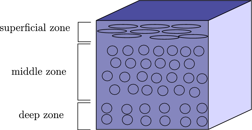
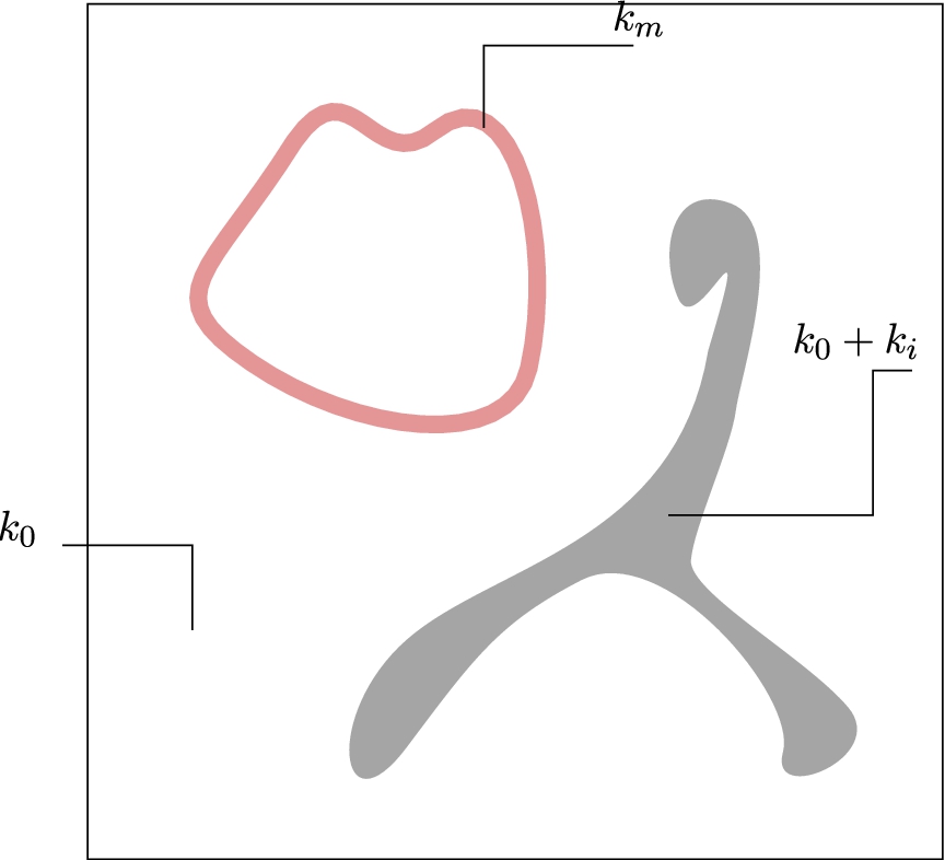
Fig. 2.
Typical values of
Now that we have an expression for the conductivity in the medium, as commonly accepted in EIT, we use the quasistatic approximation for the electrical potential. For an input current
Remark 1.
Let us briefly explain how the expression of
2.2.Homogenization of the tissue
We are now interested in getting rid of the microscale oscillations of
3.Imaging the microstructure from effective conductivity measurements
In this section, we do not care about the space dependence of
3.1.Effective conductivity in the dilute case
Here, we consider some reference cell
The effective conductivity is therefore expressed as
Theorem 2.
Let
We begin be reviewing properties of periodic layer potentials. Let us define the periodic Green’s function
Lemma 3.
We have the following jump relations along the boundary
We denote by
Theorem 4.
We have the following representation for
Lemma 5.
For any
Proof.
As shown in the Appendix,
We can now proceed to prove Theorem 4.
Proof.
Let
We now proceed to compute the representation of the effective conductivity.
Theorem 6.
We have the following representation for
Proof.
We recall the expression of
We turn to the proof of Theorem 2. We first review asymptotic properties of the periodic Green’s function
Lemma 7.
We have the following expansion for
Using this expansion, we obtain by exactly the same arguments as those in [3, Chapter 8] the following expansion, which is uniform in
3.2.Spectral measure of the tissue
Expansion (9) yields
Lemma 8.
Proof.
Let
From this result, we can now proceed. From the spectral theorem, there exists a spectral measure E such that for any
Since
Proposition 9.
Let
Proof.
Identity (19) holds using the analyticity of F in a neighborhood of 0. We also have
In the following, we write
4.Inverse homogenization
4.1.Imaging of the anisotropy ratio
The anisotropy ratio (the ratio between the largest and the lowest eigenvalue of the effective conductivity tensor) depends on the frequency [2]. Furthermore, in the general case, the anisotropy orientation (the direction of the effective conductivity tensor eigenvectors) depends also on the frequency. However, in the special case where we have an axis of symmetry of a single inclusion or a cell, the anisotropy orientation is independent of the frequency.
We denote by
Lemma 10.
Let
Proof.
We have, for any
The following corollary holds immediately.
Corollary 11.
Let
Let us begin with the two-dimensional case.
Proposition 12.
Let
Proof.
We have
We have a similar result in three dimensions. The following proposition holds.
Proposition 13.
Let
Proof.
The proof is exactly the same as in the
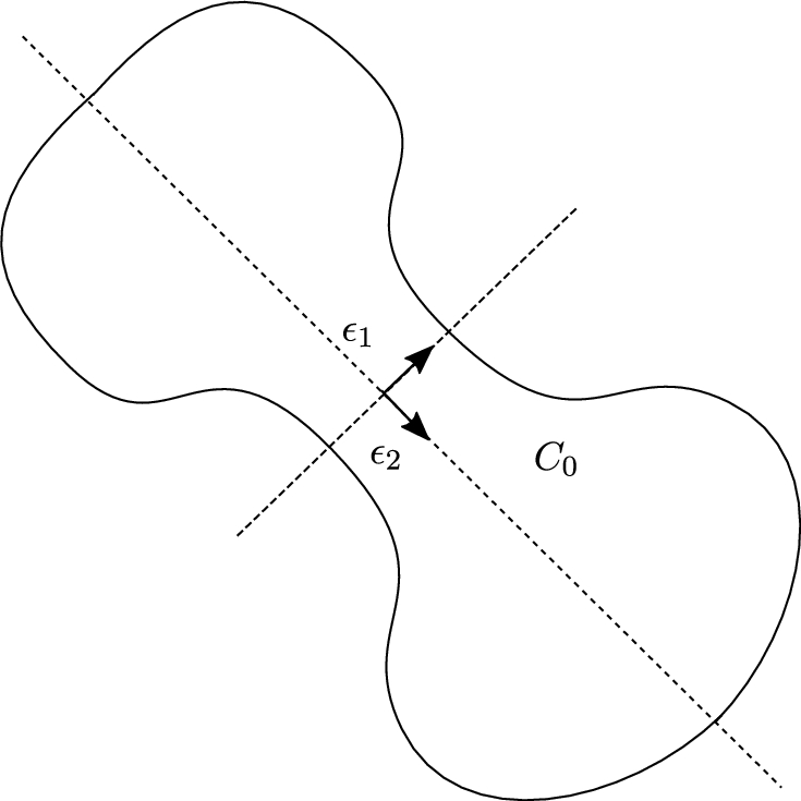
Fig. 3.
A domain presenting a symmetry. In this case, the anisotropy direction is frequency independent.
Remark 14.
It is also true that the symmetry axes of
Remark 15.
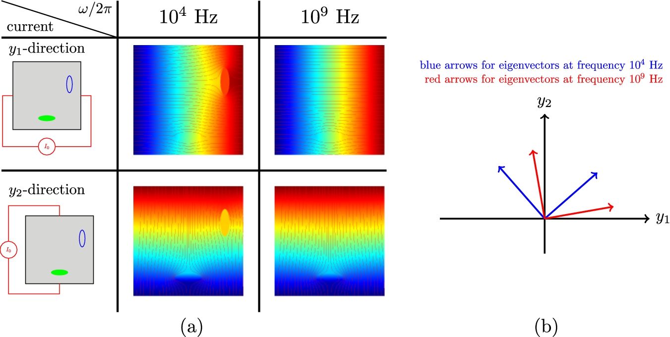
Even if each of inclusion and cell has an axis of symmetry, the direction of eigenvectors of the effective conductivity tensor can be frequency dependent. The following numerical test is conducted to show an example of frequency dependency. There are an ellipsoidal inclusion with major axis
Fig. 4.
(a) shows voltage map with current flows for each
4.2.Implementation of the inverse homogenization
Following [2], we use the following values:
The size of cells: 50 μm;
Ratio between membrane thickness and size of a cell:
Medium conductivity: 0.5 S/m;
Membrane conductivity:
Background inclusion conductivity:
Membrane permittivity:
Frequency band:
Fig. 5.
Values of
![Values of β(ω) for ω/2π∈[104;109].](https://content.iospress.com:443/media/asy/2016/100-1-2/asy-100-1-2-asy1387/asy-100-asy1387-g005.jpg)
In this case, we have values of
At each frequency, in order to compute the true effective conductivity given by (5), we perform a finite element computation using freefem
Fig. 6.
Real part of the effective conductivity.
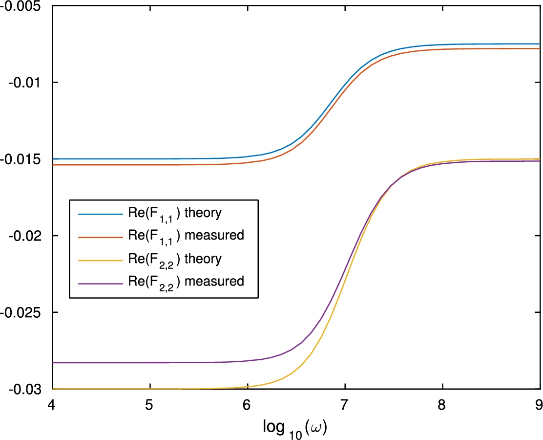
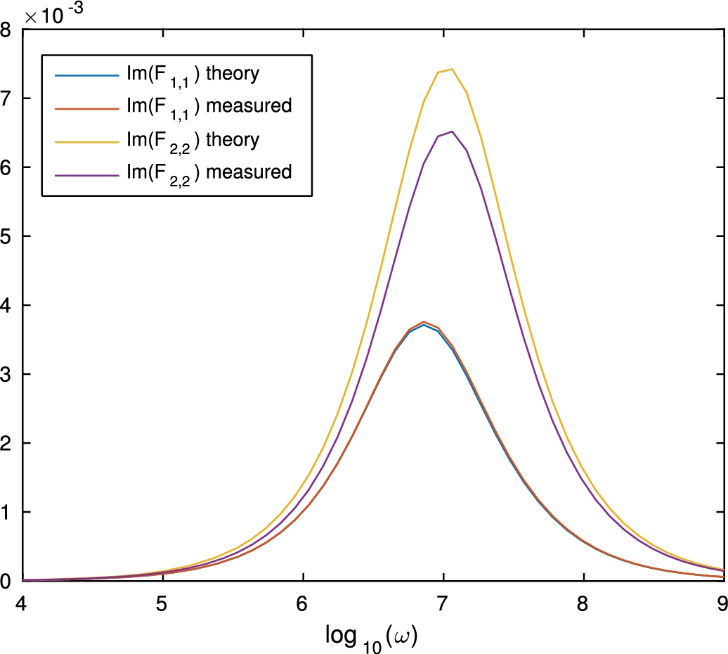
Fig. 7.
Imaginary part of the effective conductivity.
To recover the moments from the effective conductivity, we approximate as a rational function,
Numerically, this is done as a simple least square inversion: the coefficients of the polynomials
We now consider a toy example where C is an ellipse in
Since the right-hand side of (21) can be regarded as a function of
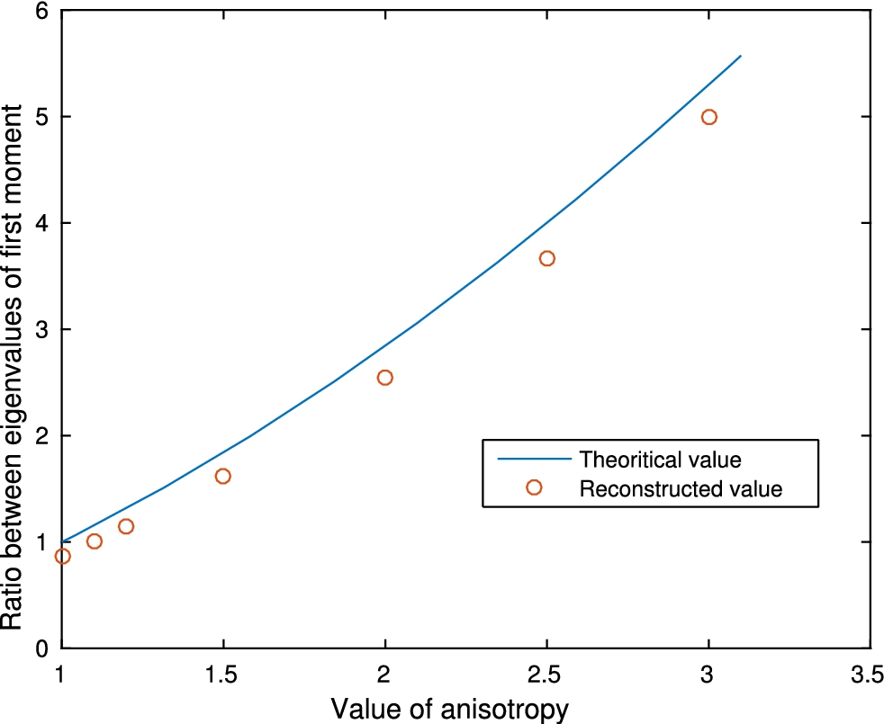
Fig. 8.
Reconstruction of r when there is no inclusion B.
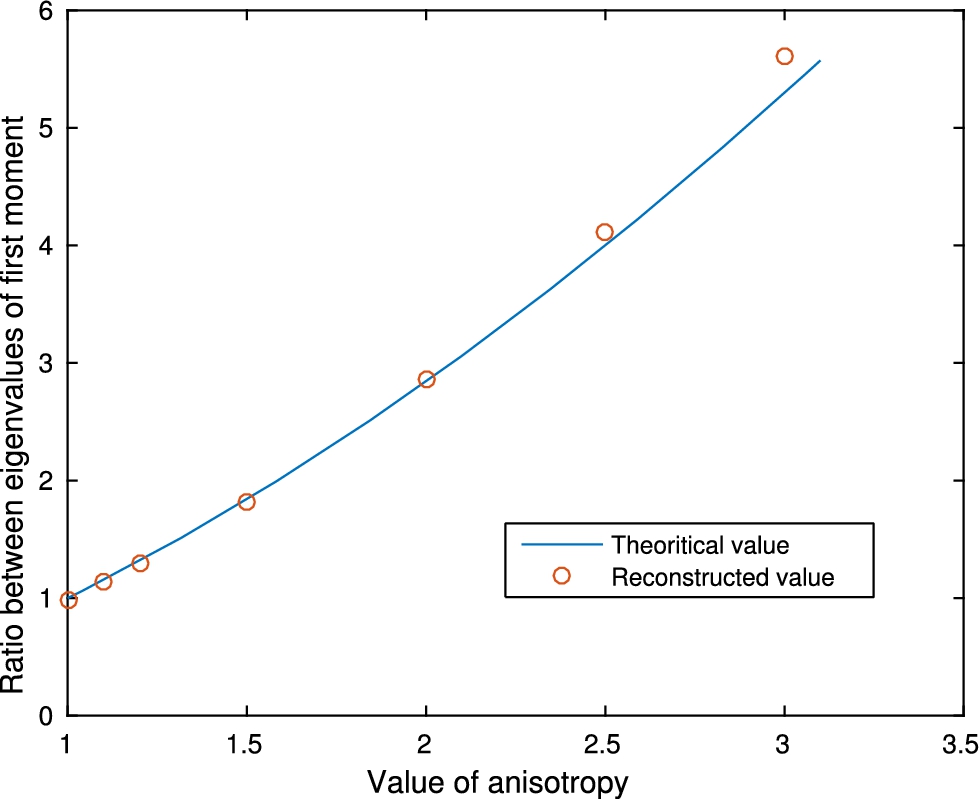
Fig. 9.
Reconstruction of r when there is an inclusion B with
After recovering the anisotropy ratio
Table 1
Reconstructed values of
| Values of | 0.01 | 0.02 | 0.03 | 0.05 | 0.1 | 0.2 | 0.3 |
| Reconstructed value | 0.0098 | 0.0196 | 0.0294 | 0.0491 | 0.0981 | 0.1963 | 0.2945 |
To reconstruct the angle of the inclusions, we simply use the orientation of the eigenvalues of the moments of
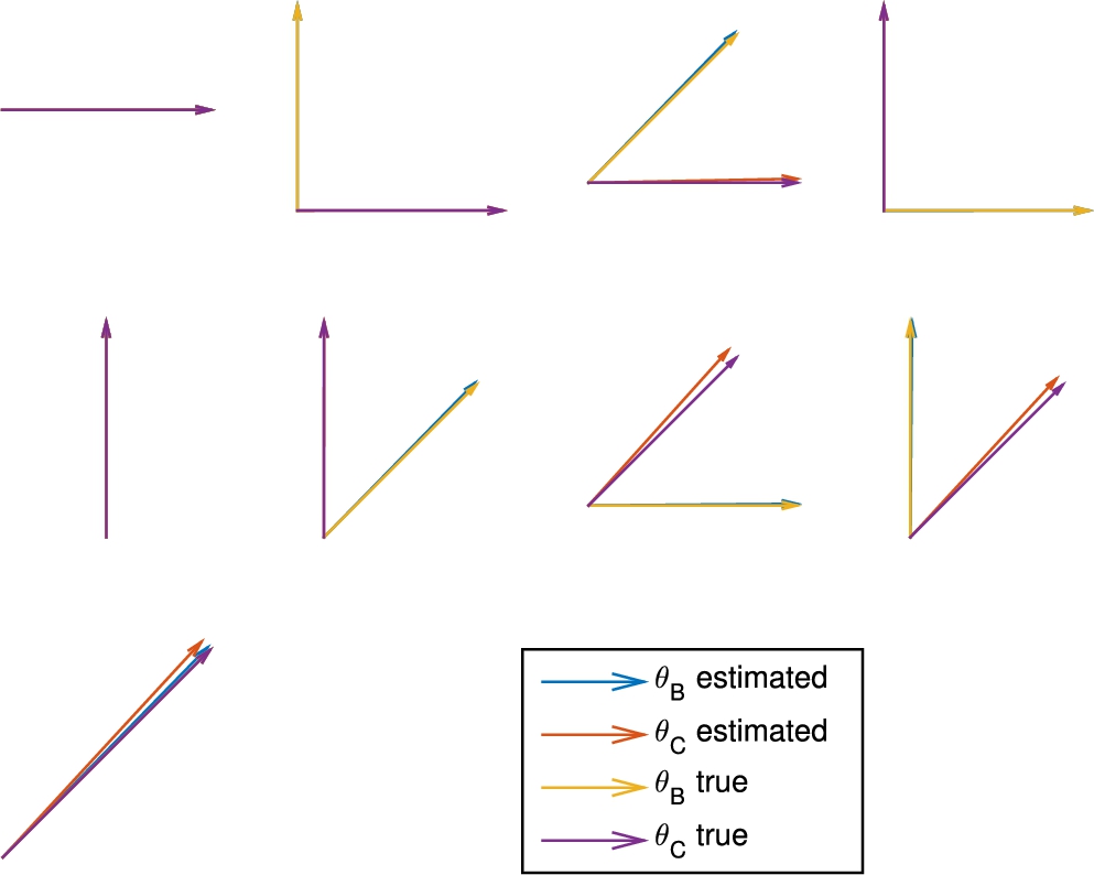
Fig. 10.
Reconstruction of the orientation of the inclusions B and C.
Appendices
Appendix
AppendixSpectrum of some periodic integral operators
Let
Theorem 16.
For any
Proof.
We first show that the operator
Theorem 17.
For
Proof.
Since
Acknowledgement
This work was supported by the ERC Advanced Grant Project MULTIMOD–267184.
References
[1] | G. Allaire, Homogenization and two-scale convergence, SIAM J. Math. Anal. 23: ((1992) ), 1482–1518. doi:10.1137/0523084. |
[2] | H. Ammari, J. Garnier, L. Giovangigli, W. Jing and J.K. Seo, Spectroscopic imaging of a dilute cell suspension, J. Math. Pures Appl. 105: ((2016) ), 603–661. doi:10.1016/j.matpur.2015.11.009. |
[3] | H. Ammari and H. Kang, Polarization and Moment Tensors. With Applications to Inverse Problems and Effective Medium Theory, Applied Mathematical Sciences, Vol. 162: , Springer, New York, (2007) . |
[4] | T.K. Chang and K. Lee, Spectral properties of the layer potentials on Lipschitz domains, Illinois J. Math. 52: ((2008) ), 463–472. |
[5] | E. Cherkaev, Inverse homogenization for evaluation of effective properties of a mixture, Inverse Prob. 17: ((2001) ), 1203–1218. doi:10.1088/0266-5611/17/4/341. |
[6] | E.B. Fabes, M. Sand and J.K. Seo, The spectral radius of the classical layer potentials on convex domains, in: Partial Differential Equations with Minimal Smoothness and Applications, Chicago, IL, 1990, IMA Vol. Math. Appl., Vol. 42: , Springer, New York, (1992) , pp. 129–137. doi:10.1007/978-1-4612-2898-1_12. |
[7] | F. Hecht, New development in freefem |
[8] | A. Khelifi and H. Zribi, Asymptotic expansions for the voltage potentials with two-dimensional and three-dimensional thin interfaces, Math. Meth. Appl. Sci. 34: ((2011) ), 2274–2290. |
[9] | S. Kim, E.J. Lee, E.J. Woo and J.K. Seo, Asymptotic analysis of the membrane structure to sensitivity of frequency-difference electrical impedance tomography, Inverse Problems 28: ((2012) ), 075004. doi:10.1088/0266-5611/28/7/075004. |
[10] | J.M. Mansour, Biomechanics of cartilage, in: Kinesiology: The Mechanics and Pathomechanics of Human Movement, Wolters Kluwer, Philadelphia, (2003) , pp. 66–79. |
[11] | G.W. Milton, The Theory of Composites, Cambridge Monographs on Applied and Computational Mathematics, Cambridge University Press, Cambridge, (2001) . |
[12] | J.-C. Nédélec, Acoustic and Electromagnetic Equations – Integral Representations for Harmonic Problems, Applied Mathematical Sciences, Vol. 144: , Springer, Berlin, (2001) . |
[13] | G. Nguestseng, A general convergence result for a functional related to the theory of homogenization, SIAM J. Math. Anal. 20: ((1989) ), 608–623. doi:10.1137/0520043. |
[14] | C. Orum, E. Cherkaev and K.M. Golden, Recovery of inclusion separations in strongly heterogeneous composites from effective property measurements, Proc. Royal Soc. A 468: ((2012) ), 784–809. doi:10.1098/rspa.2011.0527. |
[15] | C. Poignard, Asymptotics for steady state voltage potentials in a bidimensional highly contrasted medium with thin layer, Math. Meth. Appl. Sci. 31: ((2008) ), 443–479. doi:10.1002/mma.923. |
[16] | C. Poignard, About the transmembrane voltage potential of a biological cell in time-harmonic regime, ESAIM:Proceedings 26: ((2009) ), 162–179. doi:10.1051/proc/2009012. |
[17] | J.K. Seo, T.K. Bera, H. Kwon and R. Sadleir, Effective admittivity of biological tissues as a coefficient of elliptic PDE, Comput. Math. Meth. Medicine 2013: ((2013) ), 353849. |
[18] | T. Zhang, T.K. Bera, E.J. Woo and J.K. Seo, Spectroscopic admittivity imaging of biological tissues: Challenges and future directions, J. KSIAM 18: (2) ((2014) ), 77–105. |


