
A hybrid multiscale model for investigating tumor angiogenesis and its response to cell-based therapy
Abstract
Angiogenesis, a formation of blood vessels from an existing vasculature, plays a key role in tumor growth and its progression into cancer. The lining of blood vessels consists of endothelial cells (ECs) which proliferate and migrate, allowing the capillaries to sprout towards the tumor to deliver the needed oxygen. Various treatments aiming to suppress or even inhibit angiogenesis have been explored. Mesenchymal stem cells (MSCs) have recently been undergoing development in cell-based therapy for cancer due to their ability to migrate towards the capillaries and induce the apoptosis of the ECs, causing capillary degeneration. However, further investigations in this direction are needed as it is usually difficult to preclinically assess the efficacy of such therapy. We develop a hybrid multiscale model that integrates molecular, cellular, tissue and extracellular components of tumor system to investigate angiogenesis and tumor growth under MSC-mediated therapy. Our simulations produce angiogenesis and vascular tumor growth profiles as observed in the experiments. Furthermore, the simulations show that the effectiveness of MSCs in inducing EC apoptosis is density dependent and its full effect is reached within several days after MSCs application. Quantitative agreements with experimental data indicate the predictive potential of our model for evaluating the efficacy of cell-based therapies targeting angiogenesis.
1Introduction
Angiogenesis, the process in which new blood vessels are formed from existing vasculature, is an important process during growth and development, wound healing and tissue repair. In relation to tumor, angiogenesis is a crucial step that facilitates tumor advancement from benign avascular state to malignant vascular state.
During avascular state, tumor growth is supported by nutrient and oxygen supply through diffusion from the surrounding tissue. The initial rapid growth increases cell density in the tumor mass, which in turn causes the growth to slow down as the supply of nutrient and oxygen become limited. In order to sustain its continued growth, the tumor needs an independent blood supply that is acquired by recruiting new vasculature from pre-existing nearby blood vessel. Starving tumor cells release various tumor angiogenic factors, in particular the vascular endothelial growth factor (VEGF) that diffuses through the surrounding tissue and creates a chemical gradient between the tumor and its neighboring blood vessels. The lining of blood vessel is made of endothelial cells (ECs) that have cell surface receptors that bind VEGF. Upon binding with these receptors, VEGF induces ECs to degrade the parent basement membranes, creating exit sites for the ECs to migrate into the extracellular matrix towards the tumor [1–4]. This migratory movement of ECs is directed by positive chemotaxis up the VEGF gradient, as well as by haptotaxis that occurs along positive gradients of cellular adhesion sites in the extracellular matrix [5–7]. Among many macromolecules that are present in the extracellular matrix, fibronectin has been known to be very important for cell adhesion and in directing the migration of ECs [8, 9]. During migration, ECs also proliferate and produce the additional cells necessary for the capillary sprout to grow and extend towards the tumor [3]. It has been observed that some sprout tips may split and branch out, while some may fuse together forming a closed loop. This merging process is called anastomosis. As newly formed capillaries approach the tumor, the frequency of tip branching increases and the capillaries eventually penetrate the tumor to establish vascularization and bring in the needed oxygen supply into the tumor and its surrounding tissue.
Various cancer treatments have been explored with the ultimate goal of suppressing its growth and spreading. Recently, mesenchymal stem cells (MSCs) have become a topic of great focus in this aspect. While some studies reported that MSCs favor tumor growth, growing evidence suggested the potential of MSCs in suppressing tumorigenesis [10–13]. Specifically, studies reported that secretome, a broad panel of proteins secreted by MSCs, promotes apoptosis and autophagy of cancer cells in concentration and time-dependent manner [14, 15]. Alternatively, the use of MSCs in cell-based therapy comes from its ability to block the formation of new blood vessel by acting on ECs that form new capillary sprouts. Experiment by Otsu et al. shows that MSCs can cause EC apoptosis and degeneration of the capillaries [16]. Upon direct inoculation into the EC-derived capillaries, MSCs show the tendency to migrate towards ECs, intercalate between ECs, and establish Cx43-based intercellular gap junctional communication with the ECs. Subsequently, MSCs increase the ROS production that starts off the apoptosis signaling cascade, which consists of two major pathways, the mitochondria-mediated pathway and the FasL-dependent pathway. Evidence shows that these two pathways are connected and affect one another, and both converge into the activation of caspase 3 protein leading to cellular apoptosis [17–20].
Understanding the complex dynamics of MSC-induced apoptosis on ECs can immensely provide anti-angiogenesis therapeutic potential. Despite numerous experimental studies, the underlying biological mechanism of EC apoptosis is not yet fully understood. Laboratory experiments are usually cell specific and may be costly and challenging to perform. Computational model that simulates MSC-induced apoptosis can provide insight into this process as well as general virtual solution that could complement experimental methods.
Various modeling techniques have been used to simulate angiogenesis [21–28]. Continuous models consider the interactions between EC density and chemical concentrations that influence cell migratory direction. These models employ a system of nonlinear partial differential equations describing reaction-diffusion-convection of cells and their micro-environmental elements [22, 23]. Even though continuous models are more computationally cost efficient, they can only capture large-scale features of angiogenesis. On the contrary, discrete models, such as cellular automata, extended Potts, and agent-based models can better capture single-cell phenomena and finer processes of angiogenesis, such as EC sprout branching and anastomosis, on a smaller scale. This provides greater qualitative insight into the nature of the system at the expense of higher computational costs. Hybrid discrete-continuous models are developed to maximize advantages of both implementations within the same simulation. Many discrete models for angiogenesis are multiscale models that typically include the tissue scale for modeling vasculature formation. Some of the models [26, 27, 29] investigate tumor growth under various anti-tumor treatments, such as tyrosin kinase inhibitors (TKI), Dox and Sunitinib drugs, and MSC-derived secretome. However, to the extent of our knowledge, none of the previous modeling work has specifically investigated tumor response to MSC-based therapy that focuses on suppressing angiogenesis.
Our previously developed multiscale agent-based model has successfully simulated avascular tumor growth [29]. The model included molecular, cellular, and extracellular components of the tumor system, where the agent dynamics are influenced by the molecular and microenvironmental factors whose distributions are governed by a set of reaction-diffusion equations. In this paper, we extend the model to the tissue level in order to integrate an angiogenesis module and the MSC-EC interaction dynamics. At the molecular level, a system of ordinary differential equations regulates proteins expression that are involved in the apoptosis signaling pathways of the ECs.
Following the experiment by Otsu et al., we choose melanoma tumor cells as our model system. The simulation results produce morphologically similar patterns of capillary network formation and tumor growth dynamics as observed in the experiments. The model verifies and obtains a good quantitative agreement with the experimental data in [16] in investigating the role of MSCs in inducing apoptosis of the ECs and suppressing vascular tumor growth. Simulation results provide some indications that the efficacy of MSCs in suppressing angiogenesis is density dependent and further show that the full effect of MSC-therapy is reached within a few days after the treatment begins.
2Materials and methods
The model we propose here includes three types of cell agents: tumor cells, ECs and MSCs, and spans across four biological scales: molecular scale, cellular scale, tissue scale, and extracellular scale, that are closely integrated.
Tumor cells are the main agents at the cellular scale. In this level, the migration, proliferation and phenotypic switch of tumor cells as a response to oxygen availability are modeled using discrete equations. The tissue scale focuses on angiogenesis with ECs as the building blocks for capillary network formation. The dynamics of MSCs that play a role as the anti-angiogenic factor are also described in this level. Bridging the cellular and tissue levels, we have the extracellular scale that regulates the dynamics of microenvironmental components, such as oxygen, VEGF, extracellular matrix (ECM) and matrix-degradative enzyme (MDE). Lastly, the molecular scale describes the apoptosis signaling network for ECs that is initiated upon direct contact with the MSCs.
2.1Extracellular scale: reaction-diffusion for biochemical concentration
Cells interact and respond according to the changes that occur in their microenvironment. A system of four partial differential equations (PDEs) is employed to model the changes in the concentrations of oxygen, VEGF, MDE, and ECM over time. The description of the parameters used in these equations and their values are given in Table 1 in the Appendix. We use parameter values that are obtained from experiments as much as possible. The parameters whose data are not available are estimated to achieve best possible agreement with experimental results.
A unit square [0, 1] × [0, 1] is used as simulation domain and is discretized into grids of uniform size dx = dy = 0.005, which is equivalent to 10 μm. Hence, this domain corresponds to a tissue region with size 2mm × 2mm. One simulation time step is equivalent to 2 hours. Microenvironmental PDEs described below are solved numerically by using finite difference method. The homogeneous Neumann boundary conditions for the PDEs are applied by assuming zero flux along the domain boundary. The choice for this type of boundary condition is based on the assumption that the microenvironmental entities remain within this domain.
Oxygen concentration: Oxygen is one of the most critical factors that determines tumor viability. Oxygen is assumed to permeate through blood vessels, diffuse into the extracellular microenvironment, decay naturally over a long period of time, and is consumed by tumor cells. The evolution of oxygen concentration u (x, t) is given by the following reaction-diffusion equation:
(1)
At any given point x in the medium, the individual tumor cell’s uptake rate is a function of cell’s position xk and it declines exponentially as distance to x increases. Since a tumor cell whose radius is approximately 10 μm may occupy several grid points in the simulation domain, the exponential form of the uptake rate provides an efficient way to model the decrease of oxygen concentration at these grid points. The parameter ε in the second term, for instance, can be interpreted as the degree of localized oxygen consumption, which can be set small enough so that the consumption is very close to 0 at the location that is far from the tumor position xk.
The compound parameter qu is defined as qu = 2pu/r with pu denotes the vessel permeability for oxygen and r is the vessel radius. Cell k’s local oxygen concentration is the value u (x, t), where x is the nearest grid point to the cell’s position xk. We define a threshold value T1 for the cell’s local oxygen concentration to determine its viability status. Cell k is said to be hypoxic whenever u (x, t) ≤ T1.
The last term in (1) represents the addition of oxygen via blood vessel permeability. Here cj denotes the position of the jth blood vessel endothelial cell. The quantity ublood is the oxygen concentration in the blood inside the blood vessel, which is set to be 1, the maximum of oxygen scaled concentration u. The exponential factor is used in the last term of (1) to allow the possibility that oxygen diffuses right away into the neighboring location (grid points) as soon as it permeates from the blood vessel.
VEGF concentration: Hypoxic tumor cells secrete VEGF that diffuses into the surrounding tissue and activates ECs [7]. Once diffused VEGF reaches ECs, it induces ECs to migrate and sprout, forming new vasculature. The dynamics of VEGF concentration v including its natural decay over time can be described similarly as that of oxygen:
(2)
Matrix-degradative enzyme (MDE): Viable tumor cells produce MDE that diffuses and degrades the extracellular matrix, thus facilitating tumor migration. The rate of change of the MDE concentration m (x, t) can be expressed by
(3)
Extracellular matrix (ECM) density: Tumor cells adhere to the extracellular matrix (ECM) and require ECM for their migration. In this model, we assume that ECM consists of only macromolecules, particularly fibronectin, that is bound to the surrounding tissue. While the tumor cells produce MDE which degrade the matrix locally upon contact, ECs on the other hand secrete fibronectin. The process can be described by the following equation:
(4)
2.2Cellular scale: phenotypic switch and tumor migration
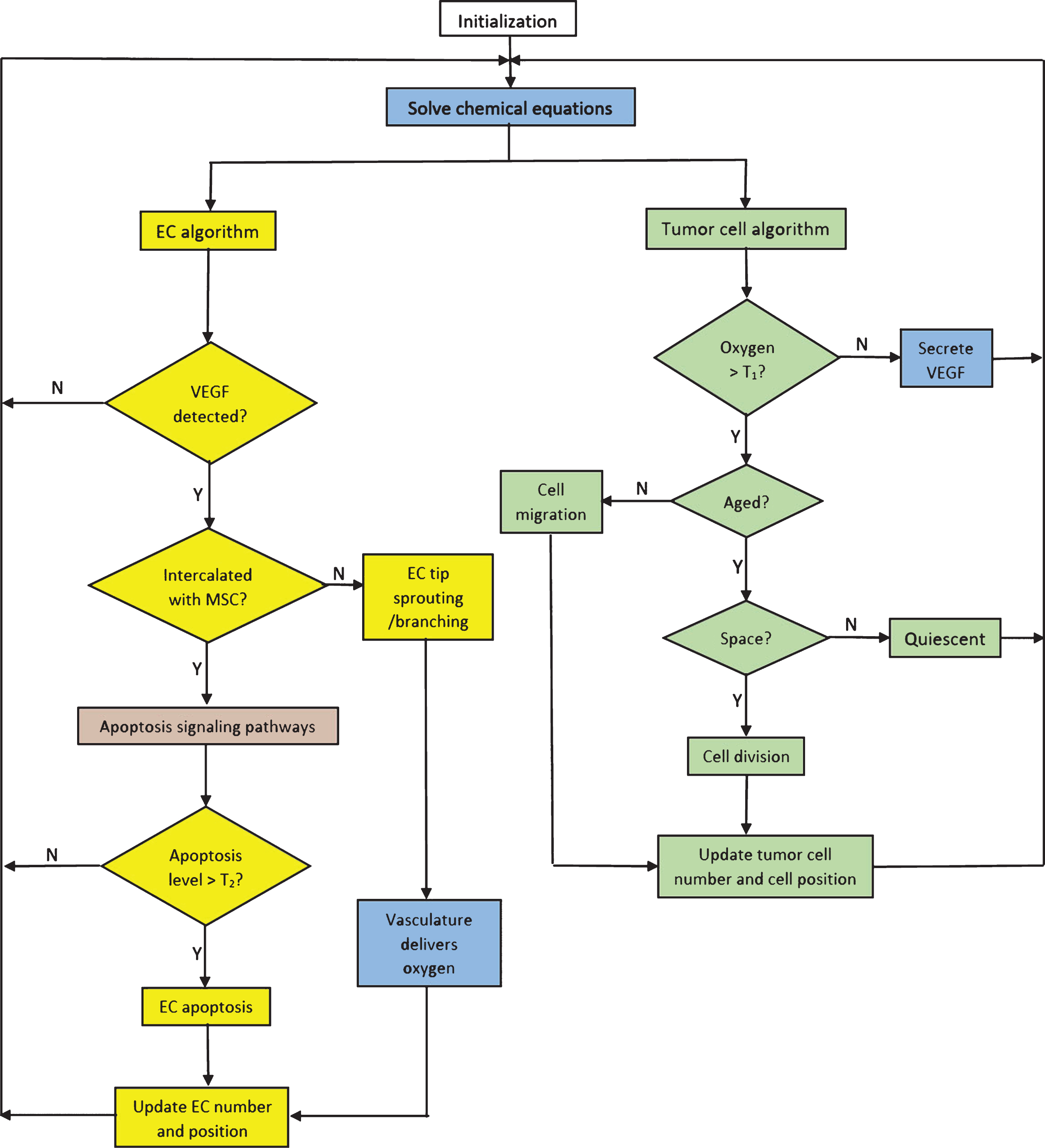
At every time step, each tumor cell agent performs a sequence of checks to determine its phenotypic switch. The following steps are depicted in the right part of the flowchart in Fig. 3 (Tumor cell algorithm):
1 Viability check
2 A tumor cell viability is determined based on local oxygen concentration. A hypoxic cell will secrete VEGF and it can neither divide nor migrate. On the other hand, if a cell is viable, it proceeds to the next check, the proliferation check.
3 Proliferation check
4 Before a viable cell can perform mitosis, it needs to check the following: (a) whether it has reached a certain age and (b) whether free space is available. Age check ensures that the cell has completed all stages in its cell cycle. For melanoma, the average doubling time is approximately 21 hours [30]. Next it checks whether there is sufficient space in its surrounding for the daughter cell to occupy. If both checks are satisfied, mitosis is performed. The parent cell stays at its current position and the new daughter cell takes the available space adjacent to the parent cell’s position. If there is insufficient space, the cell will become quiescent. A cell that has not yet mature will migrate following the algorithm that will be discussed below.
5 Cell migration
6 Tumor cell migratory direction within the microenvironment is governed by the intercellular adhesion and haptotaxis. The intercellular potential U between two distinct cells is computed as the difference between their adhesion and repulsion forces as defined in [29, 31, 32]:
where CA, CR define the adhesion and repulsion strengths, and lA, lR their effective length scales, respectively [33]. The velocity direction of cell k is then determined by summing up all the interaction potential gradients with all other cells:(5)
where Uk,j is the potential force between cells k and j.(6)
Haptotaxis is a directed migratory response of cells to gradient of fixed non-diffusible chemicals. In the case of tumor, the migrating cells choose pathways with the highest availability of ECM proteins, such as fibronectin, and adhere to it [34–36]. Hence, we define haptotaxis movement to be the upward movement of cells along the gradients of fibronectin:
with ξ denotes the haptotaxis coefficient.(7)
Combining these biasing factors, the migratory direction V (t) can be computed as their weighted average:
where the subscripts I and H refer to intercellular forces and haptotaxis, respectively, and d is their respective weights. At each time step the cell position is updated according to the discrete equation(8)
with v denotes the step length and Δt the time step.(9)
The list of parameters used in the cellular level of the model are listed in Table 2 in the Appendix.
2.3Tissue scale: angiogenesis and anti-angiogenesis
Our algorithm at the tissue scale includes: 1) growth mechanism of the capillary sprout from pre-existing blood vessel towards the tumor, 2) migration of MSCs towards EC-derived capillaries to induce apoptosis. We divide the tissue domain connecting parent blood vessel and the tumor (VEGF source) into two-dimensional grid and implement biased random walk for the movement of both ECs and MSCs on the grid points.
2.3.1Capillary growth
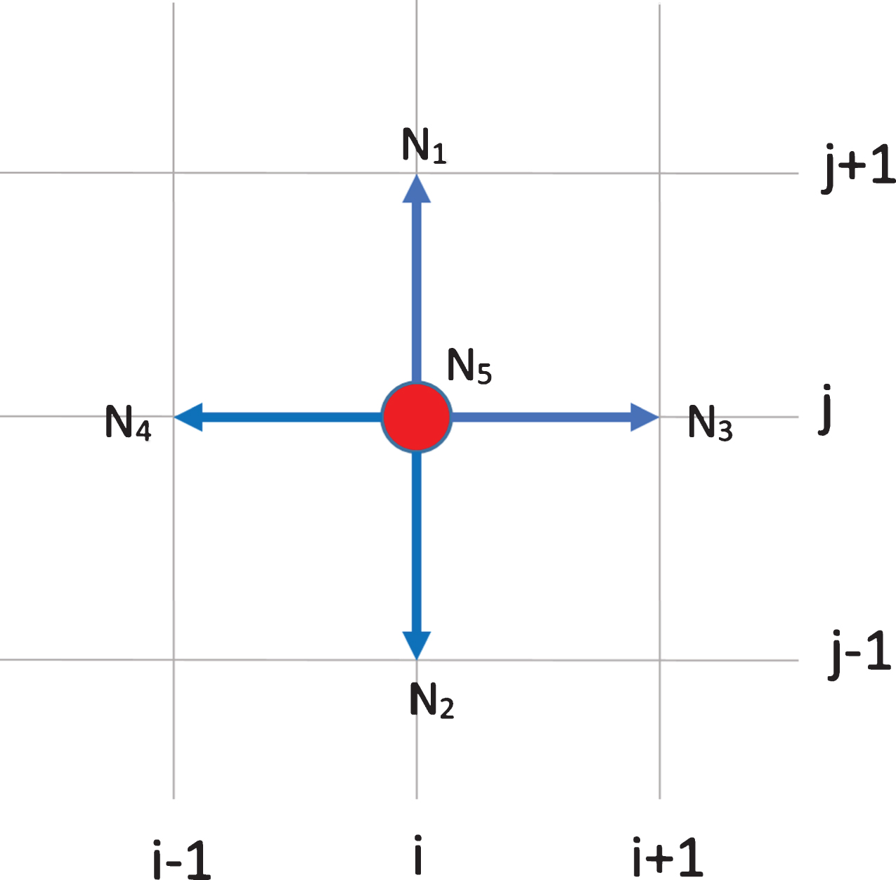
We assume that the motion of EC located at the tip of capillary sprout determines the motion of the whole sprout. This is based on fact that the ECs that line the sprout wall are contiguous [7]. At each time step, an EC at the grid point (i, j) has four orthogonal neighboring locations to move to: up N1 (i, j + 1), down N2 (i, j - 1), right N3 (i + 1, j), left N4 (i - 1, j), or stays in the current position N5 (i, j). See Fig. 1. As proposed in [22, 27], the probability Pk for the EC to move to Nk is computed according to the formula
(10)
(11)
(12)
Fig.1
Grid setting for tip endothelial cell and mesenchymal stem cell migration. At the current position (i, j), a cell has four orthogonal neighboring locations N1, N2, N3, N4 to migrate to, or stay stationary at N5.
In addition to the above migratory direction probability, we also compute the branching probability for EC sprout tip. During branching process, an EC sprout tip will split into two tips and take on two distinct neighboring locations. One phenomenon that is commonly observed in experiments is the brush border effect, where very little branching occurs when the sprout tip is far away from the tumor, and as the sprout tip is getting closer to the tumor, the branching frequency increases significantly. To produce such effect in our simulation, we use a technique similar to the positional information approach as described in [22, 37]. In particular, we impose a rule that the probability of a sprout tip to branch out increases as its distance to tumor decreases, and subsequently as its local VEGF concentration increases. Since a cell can only assess its local environment and cannot perceive how far away it is from the tumor, we define the branching probability as an increasing function of local VEGF concentration v. Such function can be chosen on qualitative basis and as an instance, the function that we use in our simulation is
(13)
Another feature that is observed in the experiment is anastomosis, the formation of loops by capillary sprouts. When two sprouts encounter each other, a loop is formed and only one sprout continues to grow. To summarize the algorithm, each EC sprout tip at location (i, j) performs the following steps:
1 EC checks if its local VEGF concentration is positive. If it is, we set the sprout tip as active and ready to migrate. Otherwise, it stays quiescent.
2 Check if EC has encountered MSC. If it has, start the apoptosis signaling (molecular scale). If not, proceed to step 3.
3 Compute the migratory direction probability (10) for each of the orthogonal neighboring sites and its associated intervals Ik.
4 Compute the branching probability (13) and generate a random number r ∈ (0, 1). We have two possible cases:
(a) Case 1: r ≤ Pb. The sprout tip branches out into two tips. We generate two random numbers s1 and s2 between 0 and 1. The branching direction is determined based on which intervals Ik these random numbers belong to. For example, if s1 ∈ I1 and s2 ∈ I3, then the first tip moves up to N1 and the second tip moves to the right to N3.
(b) Case 2: r > Pb. The sprout tip migrates to an adjacent location. We generate a random number s ∈ (0, 1) and check the interval. If s ∈ I3, then we move this EC tip to the grid point that is to the right of its current location.
5 Check if two sprouts encounter each other (anastomosis). If so, we pick randomly which sprout will continue to grow and deactivate the other one.
2.3.2MSC migration
The algorithm for MSC migration also uses similar idea of biased random walk as in the EC migration. Experiments have found that adhesion to fibronectin facilitates MSC migration in the absence of growth factor stimulation [38]. At each time step, the MSC checks its four neighboring orthogonal locations for availability. The migratory direction probability is computed based on its fibronectin gradient:
(14)
2.4Molecular scale: apoptosis signaling pathways
MSC intercalation triggers an increase in the ROS production. Literature study indicates that the two major apoptosis signaling pathways that are activated by ROS production are the mitochondrial pathway and the FasL-dependent pathway [39, 40]. The schematic model of these pathways used in this paper is shown in Fig. 2.
Fig.2
A schematic model of the apoptosis signaling pathways. 1) The mitochondrial pathway and 2) the FasL-dependent pathway mediated by NF-κB. Each pathway activates its own initiator caspase (caspase 8 and 9) which in turn will activate the executioner caspase 3.
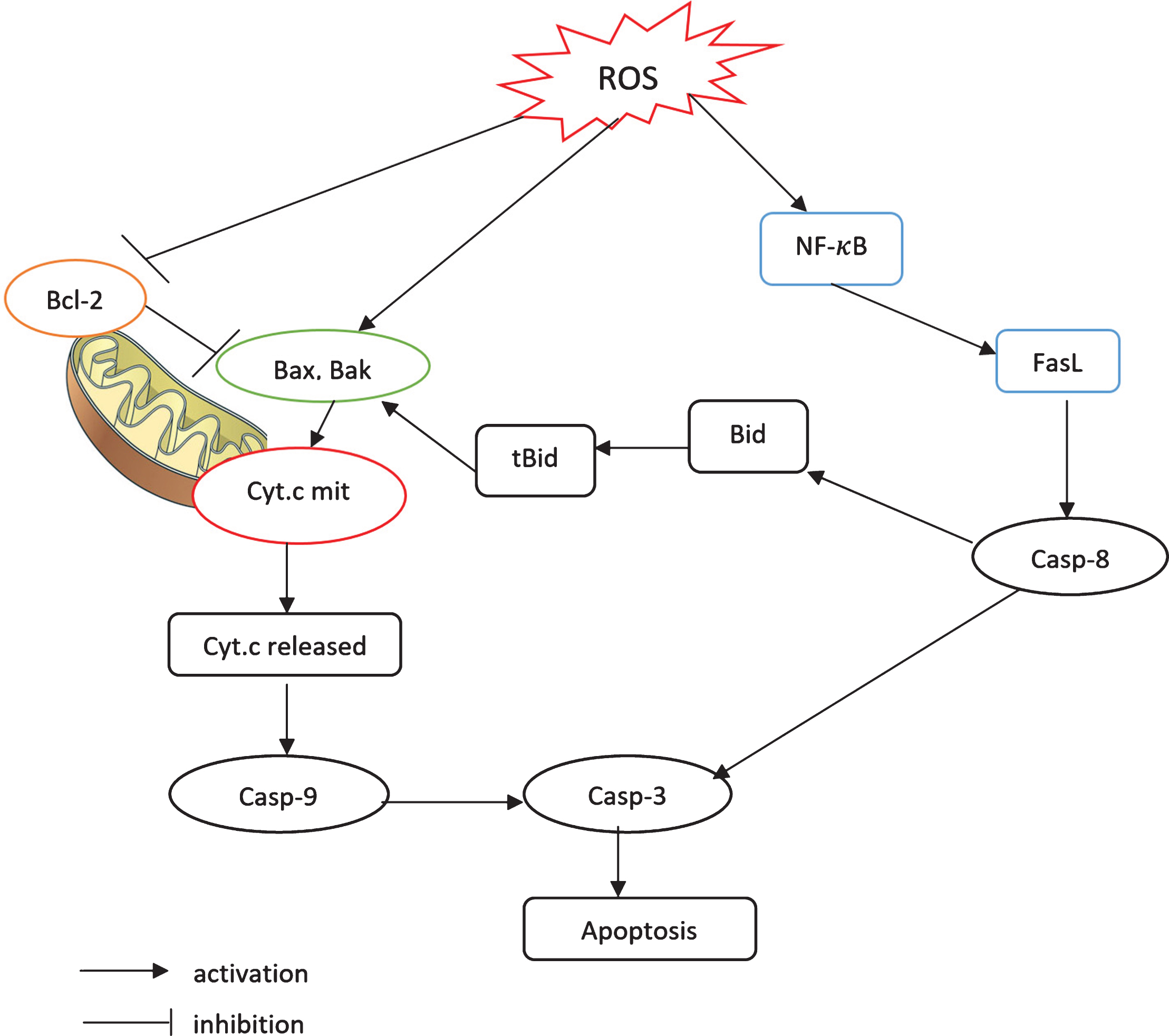
As a response to the elevated ROS level, the pro-apoptosis proteins, such as Bax and Bak, will be activated, while the anti-apoptosis proteins, such as BCl-2, will be suppressed. The activation of Bax and Bak leads to the opening of mitochondrial permeability transition pore, which triggers the release of cytochrome c from mitochondria into the cytosol [41–44]. The released cytochrome c binds and activates caspase 9. Activated caspase 9 cleaves and further activates caspase 3, which is known as the apoptosis executor protein.
Furthermore, ROS also promotes the expressions of NF-κB and FasL, which lead to the downstream activation of caspase 8. Activated caspase 8 can trigger the mitochondrial pathway through the cleavage of Bid. tBid, the truncated Bid, further stimulates Bax and Bak. Caspase 8 can also bypass the mitochondrial pathway by directly initiating the activation of caspase 3 [18, 45].
The biochemical kinetics involved in the model in Fig. 2 are given in Table 4 and their corresponding system of ordinary differential equations (ODEs) are listed in Table 5 in the Appendix. The reaction rate constants and initial values of the apoptosis proteins used in the simulation are given in Tables 6–7, respectively.
To capture intracellular variations among cells, we set the initial condition of each apoptosis protein to be a uniformly random number between 0 and 1 for simplicity. The activated state of the proteins as well as their compounds are initially set to 0. As we have not yet found any experimental data that can be used to estimate the production and decay rates of these proteins once the apoptosis signaling cascade begins, we do not include the production and decay in our model, although such possibilities may occur in sufficiently long period of time. Due to such initial conditions, very few cells may perhaps be immune from apoptosis and survive the MSC therapy. Similar phenomenon is observed in the experiment although the cause is still unclear. The apoptosis model we use here is adopted with minor modifications from our previously developed model [29], where sensitivity analysis had been performed to demonstrate the overall robustness of the model.
The integration of the molecular, cellular, tissue, and extracellular time scales and the sequence of steps computed by each agent at every iteration are illustrated in Fig. 3. In the flowchart, the extracellular level processes are colored in blue, molecular level in beige, cellular level in green and tissue level in yellow. Nondimensionalization is performed to simplify the model equations and reduce the number of parameters.
The algorithm is implemented in C++ programming language, while data visualization and analysis are done in Matlab.
Fig.3
Flowchart showing the integration of molecular, cellular, tissue and extracellular scales into a sequence of events executed by a tumor cell and an EC at each iteration. The molecular level processes are shown in beige, cellular level in green, tissue level in yellow, and extracellular level in blue.
3Results and discussion
We run several sets of simulations to test the accuracy of the proposed algorithm at every stage. In the first simulation, we test the angiogenesis algorithm at the tissue level and verifies the capillary network formation with similar patterns as those commonly observed in experiments, such as sprouting, branching and anastomosis. The second set of simulations test the accuracy of our apoptosis signaling model at the molecular level. We do this by adding MSCs into the established capillary networks and quantify the effectiveness of MSCs in inducing apoptosis of the endothelial cells. In the last set of simulations, we integrate our algorithm for tumor growth dynamics and angiogenesis with apoptosis signaling network to produce vascular tumor growth patterns and predict the effect of MSC in tumor growth.
3.1Capillary network formation patterns
The simulation domain [0, 1] × [0.1] is set up as follows: the parent blood vessel is placed on the left boundary along the line x = 0 and line tumor as source of VEGF on the right boundary along the line x = 1. We place 6 tips endothelial cells along the parent blood vessel. Taking the value from the experiment [46], we take the distance between the tumor source and parent vessel to be approximately 2mm, which is equivalent to one unit length in our simulation.
As suggested in [22, 47, 48], we take the initial VEGF concentration to be:
(15)
Fig.4
Numerical simulation of angiogenesis.(a)-(d) Spatio-temporal evolution of capillary network during the first 600 hours after VEGF reaches the parent blood vessel. The initial VEGF source is a line tumor along x = 1 and the parent blood vessel is located along the left boundary x = 0. As capillary network approaches the tumor source, the probability of branching increases and the formation of brush border becomes more evident. (e)-(f) The distribution of VEGF and fibronectin after 600 hours.
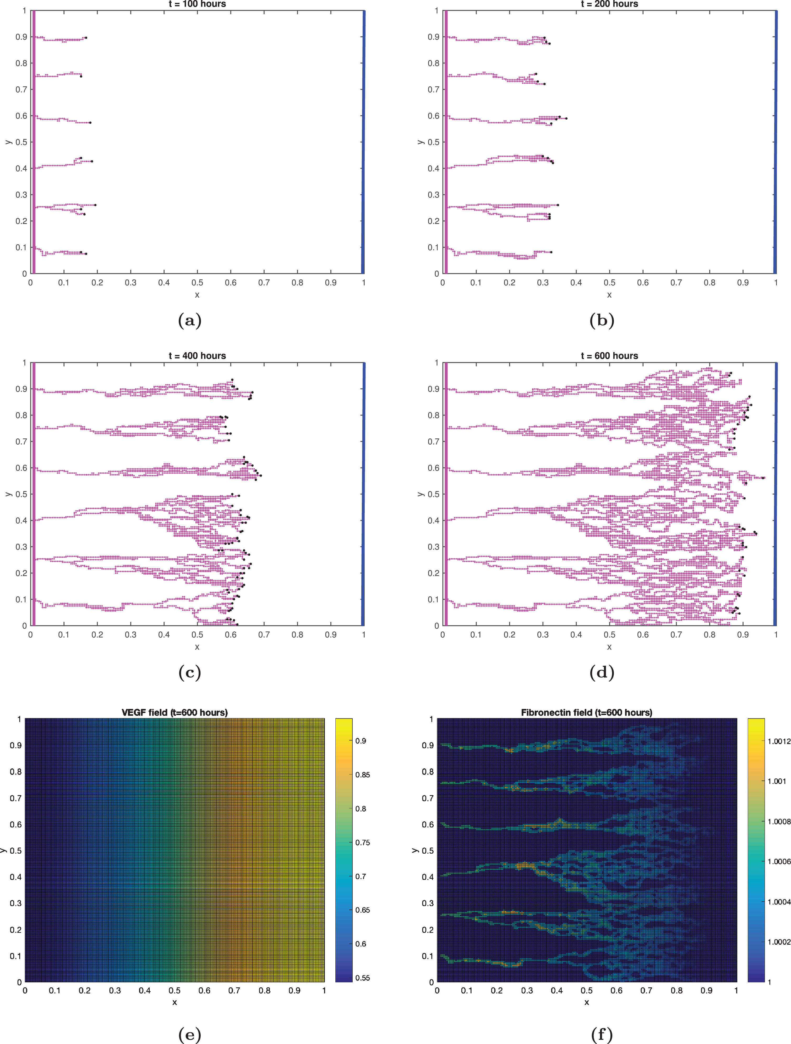
We implement the algorithm for capillary network formation described in 2.3.1. Fig. 4(a)-(d) show four snapshots of the capillary sprouts progression towards the tumor after 100, 200, 400, and 600 hours. Initially the sprouts arising from the parent vessel grow almost parallel to each other and very little branching occurs (Fig. 4a). As the sprout extends towards the tumor, where VEGF concentration is the highest, the possibility of branching increases. Due to haptotaxis, the sprouts also tend to incline toward each other and cause anastomosis. See Fig. 4(b). Fig. 4(c)-(d) show that the frequency of branching becomes more prominent as distance from tumor decreases. All six initial sprouts are eventually drawn towards the maximum VEGF concentration creating the brush border effect. This sprouting, branching and anastomosis patterns are commonly observed in the experiments [3]. Figures 4(e)-(f) show the distribution of VEGF and fibronectin at the end of t = 600 hours.
3.2MSC-induced apoptosis of endothelial cells
We now test the accuracy of apoptosis signaling network proposed in section 2.4 and the algorithm for MSC migration in section 2.3.2. For this purpose, we start with the established capillary network resulted from our first simulation (Fig. 4(d)) and spread MSCs uniformly across the simulation domain (Fig. 5(a)). Each EC is equipped with apoptosis signaling network whose equations are listed in Table 5 and their apoptosis proteins are set according to the values in Table 7. Each MSC performs biased random walk with haptotaxis movement along the gradients of bound extracellular matrix (fibronectin) as described in equation (14). Since active ECs secrete fibronectin, this results in the tendency of MSCs to migrate towards ECs. MSC is intercalated with an EC when they occupy the same location and they are shown in darker dots in Fig. 5(b). The ROS production begins for those ECs that have been intercalated with an MSC. It was known from experiments that MSC-induced ROS production increases progressively over time although there is not enough data that can be used to precisely quantify the production rate. For simulation purpose, we let each intercalated EC to increase its ROS level at each time step by a random number between 0 and 0.05. The cumulative ROS level from all ECs that have been intercalated with MSCs are shown in Fig. 5(e). When its ROS level ([ROS]) increases, a cell starts the cascade of molecular events described by the system of ODEs in the apoptosis signaling pathway in Table 5. The cell’s apoptosis level ([Apop]) is calculated by solving the system and it is set to be apoptotic when [Apop]>0.002. This apoptosis threshold is calculated using the same technique described in [29]. In Fig. 5(c)-(d) apoptotic ECs in days 3 and 5 are shown as black dots on the capillary network. There is not much difference in the EC profiles between these two days indicating that in most cases apoptosis has taken place by day 3.
Fig.5
Effect of MSC inoculation to angiogenesis. (a) The MSCs (green dots) are spread uniformly. (b) MSCs migrate toward ECs. The darker dots in the capillary network are the MSCs that have intercalated with EC on day 1 after inoculation. (c) Apoptotic ECs are shown in black dots. (d) On day 5 after MSC inoculation, there is no significant increase in the number of apoptotic ECs compared to those on day 3. (e) The cumulative ROS level on ECs increases rapidly during the first 2 days, but slows down afterwards. (f) The percentage of the surviving ECs during the first 5 days after MSC inoculation into the established capillaries. The experimental data from [16] with EC:MSC =1:1 during the first 3 days are shown in red asterisk (*).
![Effect of MSC inoculation to angiogenesis. (a) The MSCs (green dots) are spread uniformly. (b) MSCs migrate toward ECs. The darker dots in the capillary network are the MSCs that have intercalated with EC on day 1 after inoculation. (c) Apoptotic ECs are shown in black dots. (d) On day 5 after MSC inoculation, there is no significant increase in the number of apoptotic ECs compared to those on day 3. (e) The cumulative ROS level on ECs increases rapidly during the first 2 days, but slows down afterwards. (f) The percentage of the surviving ECs during the first 5 days after MSC inoculation into the established capillaries. The experimental data from [16] with EC:MSC =1:1 during the first 3 days are shown in red asterisk (*).](https://content.iospress.com:443/media/isb/2019/13-1-2/isb-13-1-2-isb469/isb-13-isb469-g005.jpg)
Since a high number of MSCs is required to ensure its effectiveness in inducing apoptosis [16], we run the simulations with EC:MSC ratios of 1:1, 5:1, and 10:1. The percentage of surviving ECs is measured for 5 days after the addition of MSCs to the established capillaries. See Fig. 5(f). On day 1, the number surviving ECs are still 90% or above for all three cell ratios. Starting on day 2, the number of surviving ECs in the simulation with EC:MSC ratio of 1:1 has dropped to approximately 25%, much lower compared to the other two cell ratios. On day 3 and onward, the limiting percentages of surviving ECs are approximately 12%, 60% and 78% for EC:MSC ratios of 1:1, 5:1 and 10:1, respectively. In all three cell ratios, we can see that the reduction in the number of surviving ECs stops at around day 3. One possible explanation to this is that even though MSCs can migrate towards the ECs, they do not travel far within the extracellular matrix. The haptotaxis driven movement is only effective locally as fibronectin secreted by ECs does not diffuse, but instead is bound to the extracellular matrix. Most MSCs that are in the vicinity of an EC have already intercalated by day 3 and the rest may not reach the EC at all. The cumulative ROS level is also shown to increase rapidly during the first two days and slows down starting on day 3 onwards, indicating that there is no new intercalation that takes place after day 3.
This result suggests that the MSC-induced apoptosis is density dependent and the full effect of MSC treatment can be seen within 3 days for all EC:MSC ratios. Experimental data from [16] for EC:MSC ratio of 1:1 during the first three days after MSC treatment is also shown in Fig. 5(f). Our simulation result shows a good agreement with these experimental data, indicating the accuracy of the model at the molecular and tissue levels.
3.3Vascular tumor growth patterns
We now integrate the molecular, cellular, tissue, and extracellular levels, as shown in the flowchart in Fig. 3 to simulate the vascular growth of tumor.
We initially place 100 active and 100 hypoxic cells in the middle of simulation domain [0, 1] × [0, 1], forming a lump of cells with radius 0.1 with initial VEGF distribution
(16)
The vascularized tumor growth patterns without MSC treatment at t = 7, 10 and 17 days are shown in Fig. 6(a)-(c). In Fig. 6(a) the cells in middle part of the tumor are hypoxic (colored in blue) due to lack of oxygen, while those in outer rim are still proliferating (colored in green). The radius of the hypoxic region and the thickness of the proliferative rim is about equal at this point. The capillary network grows towards the tumor where VEGF concentration is the highest. On day 10, the radius of the hypoxic region has grown much larger compare to the thickness of the proliferative rim around it. See Fig. 6(b). By day 17, the capillary network has reached the tumor delivering the needed oxygen to continue tumor growth. A large hypoxic region in the middle of tumor mass still persists as high cell density prevents the oxygen to diffuse through. On the other hand, the outer rim of proliferative cells has grown due to reoxygenation, with more cells can be seen in the region where capillary network exists.
Fig.6
Numerical simulation of vascular tumor growth during the first 17 days and comparison with the experimental data. (a)-(b) Tumor growth profile with capillary network growing towards the tumor (VEGF source). The hypoxic cells (colored in blue) are found in the middle of the lump surrounded by proliferative cells (colored in green). (c) Due to reoxygenation, more proliferative cells can be seen in the region where capillary network exists (d) Comparison between simulation and experimental data [26, 49] on the number of cells during the first 12 days of vascular growth.
![Numerical simulation of vascular tumor growth during the first 17 days and comparison with the experimental data. (a)-(b) Tumor growth profile with capillary network growing towards the tumor (VEGF source). The hypoxic cells (colored in blue) are found in the middle of the lump surrounded by proliferative cells (colored in green). (c) Due to reoxygenation, more proliferative cells can be seen in the region where capillary network exists (d) Comparison between simulation and experimental data [26, 49] on the number of cells during the first 12 days of vascular growth.](https://content.iospress.com:443/media/isb/2019/13-1-2/isb-13-1-2-isb469/isb-13-isb469-g006.jpg)
We compute the total number of melanoma cells in the tumor mass over time and compare the simulation result with the experiments in [26, 49] on melanoma growth during the first 12 days. A good agreement shown in Fig. 6(d) validates the model.
To simulate the vascular tumor growth under MSC treatment, we place MSCs uniformly across the simulation domain on day 7, as performed in the experiment by [16]. As MSC triggers EC apoptosis, the capillary network formation is abrogated. Consequently, less oxygen will be delivered to the starving tumor, slowing down its growth. In vivo experiment by [16] compared the volumes of untreated tumor and the one treated with EC:MSC ratio of 1:1. Since our simulation is two-dimensional, we can only compute the radius r of the tumor, which is the largest distance from a tumor cell to the center of the tumor at (0.5, 0.5). Assuming the spherical shape of the tumor mass, we estimate its volume by the formula V = (4/3) πr3. Fig. 7 shows the relative volume of the tumor from our simulation and the experiment for both control group (untreated) and those treated with MSCs. The volume is scaled with respect to their volume on day 7. By day 17, both simulation and experiment show that without MSC treatment, the tumor can grow up to approximately 18-20 times their volume on day 7, while under MSC treatment, the growth can be suppressed to about half (below 10 times its volume on day 7). This indicates the effectiveness of MSC in suppressing tumor growth when given in high number.
Fig. 7
Simulation and experimental data comparison of tumor volume with and without MSC treatment. MSCs are inoculated into tumor tissue on day 7 with EC:MSC ratio of 1:1. The tumor volume during the first 17 days is measured relative to its volume on day 7. The experimental data is taken from [16].
![Simulation and experimental data comparison of tumor volume with and without MSC treatment. MSCs are inoculated into tumor tissue on day 7 with EC:MSC ratio of 1:1. The tumor volume during the first 17 days is measured relative to its volume on day 7. The experimental data is taken from [16].](https://content.iospress.com:443/media/isb/2019/13-1-2/isb-13-1-2-isb469/isb-13-isb469-g007.jpg)
4Conclusion
Understanding the mechanism of MSC-induced apoptosis of endothelial cells is important in utilizing the potential of MSC as an anti-angiogenesis agent for cancer therapy. For this purpose, we develop an algorithm for angiogenesis and incorporate it with our previously developed multiscale tumor model [29]. In addition to tumor cells, the model now includes MSCs and ECs as interacting agents whose dynamics are dependent on the spatio-temporal distributions of microenvironmental factors, such as oxygen, VEGF, fibonectin and matrix degradative enzyme.
We run sets of simulations and test our algorithm at each biological level against experimental or literature data. Our simulation is able to reproduce branching, sprouting, anastomosis, and brush border patterns of the capillary network formation as commonly observed in experiments. We further verify and quantify the efficacy of MSCs in inducing apoptosis of the EC-derived capillaries, and consequently suppressing tumor vascular growth. We implement the model in a two-dimensional setting with the aim to reduce computational cost. Both qualitative and quantitative agreements with the experiments show that the two-dimensional setting does not hinder the model potential to be used as a computational tool to predict tumor response to cell-based therapy targeting angiogenesis. The model may still have some weaknesses that we would like to improve in our future projects. One would be to include the production and decay of the apoptosis signaling proteins, so that they can reach steady state levels and continue the signal transduction when simulation time scale is fairly long. Another possible improvement would be to extend the model to three dimensions to achieve better accuracy as well as to simulate cancer metastasis.
Author contributions
M.H. developed mathematical model, wrote computer codes, performed simulations, analyzed data and simulation results. J.S. formulated biological questions, performed literature study and provided experimental data. Both authors designed the project and wrote the paper.
Appendices
Appendix
Table 1
Parameter values used in the extracellular component of the model
| Symbol | Parameter | Value | Ref. |
| Du | Oxygen diffusion coefficient | 1.75 × 10⁻⁵ cm2/s | [50] |
| γu | Tumor cell oxygen consumption rate | 6.25 × 10⁻¹⁷ M/cells/s | [51] |
| δu | Oxygen decay rate | 0* | Est. in [29] |
| ε | Degree of chemical localization | 0.1 | Est. in [29] |
| pu | Vessel permeability of oxygen | 3 × 10⁻⁴ cm/s | [27] |
| r | Blood vessel radius | 0.001 cm | [27] |
| Dv | VEGF diffusion coefficient | 2.9 × 10⁻⁷ cm2/s | [22] |
| Sv | VEGF production rate | 0.6 nM/h | [27] |
| δv | VEGF decay rate | 0.001 /h | [52] |
| pv | Vessel permeability of VEGF | 0.1 × 10⁻⁴ cm/s | [22] |
| Dm | MDE diffusion coefficient | 10-9 cm2/s | [53] |
| μm | Single cell MDE production rate | 1* | [54] |
| δm | MDE decay rate | 0* | [54] |
| δf | ECM degradation rate | 50* | [54] |
| β | Fibronectin production rate | 0.05* | [22] |
| T1 | Oxygen threshold for hypoxic state | 0.3* | Est. in [29] |
*=non-dimensionalized value.
Table 2
Parameter values used in the cellular component of the model
| Symbol | Parameter | Value | Ref. |
| r | Melanoma cell radius | 10 μm | [26] |
| CA/CR | Attraction to repulsion coefficient ratio | 0.3* | [31] |
| LA, LR | Attraction and repulsion length-scales | 0.5, 0.1* | |
| ξ | Haptotaxis coefficient | 2600 cm2/s/M | [54] |
| T | Melanoma doubling time | 20.1-21.1 hours | [30] |
*=non-dimensionalized value.
Table 3
Parameter values used in the tissue component of the model
| Symbol | Parameter | Value | Ref. |
| α | EC chemotaxis coefficient | 2600 cm2 s-1 M-1 | [22, 55] |
| λ1 | EC haptotaxis coefficient | 986 cm2 s-1 M-1 | [22] |
| λ2 | MSC haptotaxis coefficient | 986 cm2 s-1 M-1 | Est. |
| σ | Constant of VEGF chemotaxis sensitivity | 1.667 × 10⁻¹⁰* | [22] |
*=non-dimensionalized value.
Table 4
Biochemical kinetics involved in the apoptosis signaling pathways of endothelial cell upon ROS production
| FasL-dependent pathway: |
| ROS + NF-κB
|
| NF-κB* + FasL
|
| FasL* + Casp8
|
| Casp8* + Bid
|
| Casp8* + Casp3
|
| Mitochondrial pathway: |
| ROS + Bax
|
| tBid + Bax
|
| ROS + BCl2
|
| Bcl2 + Bax
|
| Bax·Bak + Cytcmit
|
| Cytc + Casp9
|
| Casp9* + Casp3
|
Notation: A* = the activated state of protein A; A·B = the compound of proteins A and B; k+ = forward rate constant of reaction; k- = reverse rate constant of reaction; Cytcmit = cytochrome c in mitochondria; Cytc = the released cytochrome c.
Table 5
The system of ordinary differential equations for the biochemical kinetics of the apoptosis signaling pathways. Blocks A and B list the equations involved in FasL-dependent and mitochondrial pathways, respectively, and block C contains the equations used in both pathways
| A | d [NF - κB]/dt = - k11 [NF - κB] |
|
| |
|
| |
|
| |
|
| |
|
| |
|
| |
|
| |
|
| |
|
| |
|
| |
|
| |
| B |
|
| d [Bax · Bak]/dt = k21 [ROS] [Bax] + k23 [tBid · Bax] | |
|
| |
|
| |
|
| |
|
| |
| d [Cytcmit]/dt = - k26 [Bax · Bak] [Cytcmit] | |
|
| |
|
| |
|
| |
|
| |
| -k31 [Casp9*] [Casp3*] | |
|
| |
| C |
|
|
| |
|
| |
| d [Casp3*]/dt = k19 [Casp8* · Casp3] - k20 [Casp8*] [Casp3*] + k30 [Casp9* · Casp3] - k31 [Casp9*] [Casp3*] | |
| d [Apop]/dt = k20 [Casp8*] [Casp3*] + k31 [Casp9*] [Casp3*] |
Table 6
Reaction rate constants for biochemical kinetics used in the simulation
| FasL-dependent pathway | Mitochondrial pathway | ||||||
| k11† | 0.5μM-1s-1 |
| 1μM-1s-1 | k21† | 0.5μM-1s-1 | k26 | 10μM-1s-1 |
|
| 1μM-1s-1 |
| 1s-1 |
| 1μM-1s-1 |
| 1μM-1s-1 |
|
| 1s-1 | k17 | 1s-1 |
| 1s-1 |
| 1s-1 |
| k13† | 1s-1 |
| 1μM-1s-1 | k23 | 1s-1 | k28 | 1s-1 |
|
| 1μM-1s-1 |
| 1s-1 |
| 1μM-1s-1 |
| 10μM-1s-1 |
|
| 1s-1 | k19 | 1s-1 |
| 1s-1 |
| 0.5s-1 |
| k15 | 1s-1 | k20 | 1μM-1s-1 |
| 1μM-1s-1 | k30 | 0.1s-1 |
|
| 1s-1 | k31 | 1μM-1s-1 | ||||
†, estimated parameters. All other values are taken from [56]. The superscript "+" indicates forward rate constant and "-" reverse rate constant. The units for reaction rate constants are μM-1s-1 for bimolecular reactions and s-1 for monomolecular reactions.
Table 7
Initial values of apoptosis proteins used in the simulation
| NF-κB | [0, 1] | NF-κB* | 0 | NF-κB*.FasL | 0 | FasL*.Casp8 | 0 |
| FasL | [0, 1] | FasL* | 0 | Casp8*.Bid | 0 | Casp8*.Casp3 | 0 |
| Casp8 | [0, 1] | Casp8* | 0 | Bax.Bak | 0 | tBid.Bax | 0 |
| Casp3 | [0, 1] | Casp3* | 0 | ROS.BCl2 | 0 | BCl2.Bax | 0 |
| Apop | 0 | Cytc.Casp9 | 0 | Casp9*.Casp3 | 0 | ||
| Bid | [0,1] | tBid | 0 | ||||
| Bax | [0, 1] | BCl2 | [0, 1] | ||||
| Cytcmit | [0, 1] | Cytc | 0 | ||||
| Casp9 | [0, 1] | Casp9* | 0 |
All values are in non-dimensional form. The value [0, 1] means a uniformly random number between 0 and 1. Notation: A* = the activated state of protein A; A·B = the compound of proteins A and B; Cytcmit = cytochrome c in mitochondria; Cytc = the released cytochrome c.
References
[1] | Gerhardt H. , Golding M. , Fruttinger M. , et al., VEGF guidesangiogenic sprouting utilizing endothelial tip cell filopodia, Journal of Cell Biology 161: ((2003) ), 1163–1177. |
[2] | Yoshida A. , Anand-Apte B. and Zetter B.R. , Differentialendothelial migration and proliferation to basic fibroblastggrowth factor and vascular endothelial growth factor, GrowthFactors 13: ((1996) ), 57–64. |
[3] | Paweletz N. and Knierim M. , Tumor-related angiogenesis, Critical Reviews in Oncology/Hematology 9: ((1989) ), 197–242. |
[4] | Terranova V.P. , Diorio R. , Lyall R.M. , et al., Human endothelialcells are chemotactic to endothelial cell growth factor andheparin, Journal of Cell Biology 101: ((1985) ), 2330–2334. |
[5] | Cao Y. , Chen H. , Zhou L. , et al., Heterodimers of placenta growthfactor/vascular endothelial growth factor: Endothelial activity,tumor cell expression, and high affinity binding to FLK-1/KDR, Journal of Biological Chemistry 271: ((1996) ), 3154–3162. |
[6] | Stetler-Stevenson W.G. , Matrix metalloproteinases in angiogenesis:A moving target for therapeutic intervention, Journal ofClinical Investigation 103: ((1999) ), 1237–1241. |
[7] | Stokes C.L. and Lauffenburger D.A. , Analysis of the roles ofmicrovessel endothelial cell random motility and chemotaxis inangiogenesis, Journal of Theoretical Biology 152: (3) ((1991) ), 377–403. |
[8] | Albini A. , Allavena G. , Melchiori A. , et al., Chemotaxis of 3T3and SV3T3 cells to bronectin is mediated through thecell-attachment site in fibronectin and fibronectin cell surfacereceptor, Journal of Cell Biology 105: ((1987) ), 1867–1872. |
[9] | Carter S.B. , Haptotaxis and the mechanism of cell motility, Nature 213: ((1967) ), 256–260. |
[10] | Cuiffo B.G. and Karnoub A.E. , Mesenchymal stem cells in tumordevelopment emerging roles and concepts, Cell Adh Migr 6: (3) ((2012) ), 220–230. |
[11] | Zimmerlin I. , Park T.S. , Zambidis E.T. , Donnenberg V.S. and Donnenberg A.D. , Mesenchymal stem cell secretome and regenerativetherapy after cancer, Biochimie 95: (12) ((2013) ), 2235–2245. |
[12] | Zhang T. , Lee Y.W. , Rui Y.F. , et al., Bone marrow-derivedmesenchymal stem cells promote growth and angiogenesis of breastand prostate tumors, Stem Cell Research and Therapy 4: (3) ((2013) ). doi: 10.1186/scrt221 |
[13] | Long X. , Matsumoto R. , Yang P. and Uemura T. , Effect of humanmesenchymal stem cells on the growth of HepG2 and Hela cells, Cell Structure and Function 38: (1) ((2013) ), 109–121. |
[14] | Gauthaman K. , Yee F.C. , Cheyyatraivendran S. , et al., Humanumbilical cord Wharton’s jelly stem cell (hWJSC) extracts inhibitcancer cell growth in vitro, Journal of Cellular Biochemistry 113: (6) ((2012) ), 2027–2039. |
[15] | Sandra F. , Sudiono J. , Sidharta E.A. , et al., Conditioned Media ofHuman Umbilical Cord Blood Mesenchymal Stem Cell-derived SecretomeInduced Apoptosis and Inhibited Growth of HeLa Cells, TheIndonesian Biomedical Journal 6: (1) ((2014) ), 57–62. |
[16] | Otsu K. , Das S. , Houser S.D. , et al., Concentration-dependentinhibition of angiogenesis by mesenchymal stem cells, Blood 113: (18) ((2009) ), 4197–4205. |
[17] | Igney F.H. and Krammer P.H. , Death and anti-death: Tumourresistance to apoptosis, Nature Reviews Cancer 2: (4) ((2002) ), 277–288. |
[18] | Cooper D.M. , The Balance between Life and Death: Defining a Rolefor Apoptosis in Aging, Journal of Clinical and ExperimentalPathology S4: ((2012) ), 001. doi: 10.4172/2161-0681.S4-001 |
[19] | Martinvalet D. , Zhu P. and Lieberman J. , Granzyme A inducescaspase-independent mitochondrial damage, a required first stepfor apoptosis, Immunity 22: (3) ((2005) ), 355–370. |
[20] | Elmore S. , Apoptosis: A Review of Programmed Cell Death, Toxicologic Pathology 35: (4) ((2007) ), 495–516. |
[21] | Nekka F. , Kyriacos S. , Kerrigan C. and Cartilier L. , A model ofgrowing vascular structures, Bulletin of MathematicalBiology 58: ((1996) ), 409–424. |
[22] | Anderson A. and Chaplain M. , Continuous and Discrete MathematicalModels of Tumor-induced Angiogenesis, Bulletin ofMathematical Biology 60: ((1998) ), 857–900. |
[23] | Chaplain M. , Mathematical modelling of angiogenesis, Journalof Neuro-Oncology 50: ((2000) ), 37–51. |
[24] | Chaplain M. and Stuart A. , A model mechanism for the chemotacticresponse of endothelial cells to tumour angiogenesis factor, IMA Journal of Mathematics Applied in Medicine and Biology 10: ((1993) ), 149–168. |
[25] | Olsen M. and Siegelmann H. , Multiscale Agent-based Model of TumorAngiogenesis, Procedia Computer Science 18: ((2013) ), 1016–1025. |
[26] | Wang J. , Zhang L. , Jing C. , et al., Multi-scale agent-basedmodeling on melanoma and its related angiogenesis analysis, Theoretical Biology and Medical Modelling 10: (41) ((2013) ). |
[27] | Sun X. , Zhang L. , Tan H. , et al., Multi-scale agent-based braincancer modeling and prediction of TKI treatment response:Incorporating EGFR signaling pathway and angiogenesis, BMCBioin-formatics 13: (218) ((2012) ). |
[28] | Plank M. and Sleeman B. , Lattice and Non-lattice Models of TumourAngiogenesis, Bulletin of Mathematical Biology 66: (6) ((2004) ), 1785–1819. |
[29] | Hendrata M. and Sudiono J. , A Computational Model forInvestigating Tumor Apoptosis Induced by Mesenchymal StemCell-derived Secretome, Computational and MathematicalMethods in Medicine ((2016) ), Article ID 4910603, 17 pages, doi: 10.1155/2016/4910603 |
[30] | Ohira T. , Ohe Y. , Heike Y. , et al., In vitro and in vivo growth ofB16F10 melanoma cells transfected with interleukin-4 cDNA and genetherapy with the transfectant, Journal of Cancer Research andClinical Oncology 120: (11) ((1994) ), 631–635. |
[31] | Abajian A.C. and Lowengrub J.S. , An agent-based hybrid model foravascular tumor growth, The UC Irvine Undergraduate Research Journal 11: ((2008) ). |
[32] | Chuang Y. , D’Orsogna M.R. , Marthaler D. , Bertozzi A. and Chayes L.S. , State Transitions and the Continuum Limit for a 2DInteracting, Self-Propelled Particle System, Physica D:Nonlinear Phenomena 232: (1) ((2007) ), 33–47. |
[33] | Levine H. , Rappel W.J. and Cohen I. , Self-organization in systemsof self-propelled particles, Physical Review E63: (2000), 017101. |
[34] | Klominek J. , Robert K.H. and Sundqvist K.G. , Chemotaxis andhaptotaxis of human malignant mesothelioma cells: Effects offibronectin, laminin, type IV collage, and an autocrine motilityfactor-like substance, Cancer Research 53: (18) ((1993) ), 4376–4382. |
[35] | Lawrence J.A. and Steeg P.S. , Mechanisms of tumour invasion andmetastasis, World Journal of Urology 14: (3) ((1996) ), 124–130. |
[36] | Debruyne P.R. , Bruyneel E.A. , Karaguni I.M. , et al., Bile acidsstimulate invasion and haptotaxis in human corectal cancer cellsthrough activation of multiple oncogenic signaling pathways, Oncogene 21: (44) ((2002) ), 6740–6750. |
[37] | Wolpert L. , Positional information and pattern formation, Philosophical Transactions of the Royal Society of London B295: ((1981) ), 441–450. |
[38] | Veevers-Lowe J. , Ball S.G. , Shuttleworth A. and Kielty C.M. , Mesenchymal stem cell migration is regulated by fibronectinthrough alpha5beta1-integrin-mediated activation of PDGFR-beta andpotentiation of growth factor signals, Journal of Cell Science 124: ((2011) ), 1288–1300. doi: 10.1242/jcs.076935 |
[39] | Shi Y. , Song Y. , Wang Y. , et al., p, p-DDE Induces Apoptosis ofRat Sertoli Cells via a FasL-Dependent Pathway, Journal ofBiomedicine and Biotechnology ((2009) ), Article ID 181282, doi: 10.1155/2009/181282 |
[40] | Jin X. , Song L. , Liu X. , et al., Protective Efficacy of Vitamins Cand E on p, p-DDT-Induced Cytotoxicity via the ROS-MediatedMitochondrial Pathway and NF-gammaB/FasL Pathway, PLoS One 9: (12), e113257. doi: 10.1371/journal.pone.0113257 |
[41] | Crompton M. , The mitochondrial permeability transition pore andits role in cell death, Biochemical Journal 341: (2) ((1999) ), 233–249. |
[42] | Green D.R. and Reed J.C. , Mitochondria and apoptosis, Science 281: (5381) ((1998) ), 1309–1312. |
[43] | Kim J.S. , He L. and Lemasters J.J. , Mitochondrial permeabilitytransition: a common pathway to necrosis and apoptosis, Biochemical and Biophysical Research Communications 304: (3) ((2003) ), 463–470. |
[44] | Kroemer G. and Reed J.C. , Mitochondrial control of cell death, Nature Medicine 6: (5) ((2000) ), 513–519. |
[45] | Tait S. and Green D.R. , Mitochondria and cell death: Outermembrane permeabilization and beyond, Nature Reviews Molecular Cell Biology 11: ((2010) ), 621–632. |
[46] | Gimbrone M. , Contran R. , Leapman S. and Folman J. , Tumor growthand neovascularization: An experimental model using the rabbitcornea, Journal of the National Cancer Insititute 52: (1974), 413–427. |
[47] | Chaplain M.A.J. , The mathematical modelling of tumour angiogenesisand invasion, Acta Bio-theor 43: ((1995) ), 387–402. |
[48] | Chaplain M.A.J. , Avascular growth, angiogenesis and vasculargrowth in solid tumours: The mathematical modelling of the stagesof tumour development, Math Comput Model 23: ((1996) ), 47–87. |
[49] | Khodadoust M.S. , et al., Melanoma proliferation andchemoresistance controlled by the DEK oncogene, Cancer Res 69: ((1996) ), 6405–6413, doi: 10.1158/0008-5472.CAN-09-1063 |
[50] | Grote J. , Susskind R. and Vaupel P. , Oxygen diffusivity in tumortissue (DS-Carcinosarcoma) under temperature conditions within therange of 20-40C, Pugers Archiv 372: (1) ((1977) ), 37–42. doi: 10.1007/BF00582204 |
[51] | Casciari J.J. , Sotirchos S.V. and Sutherland R.M. , Mathematicalmodelling of microenvironment and growth in EMT6/Ro multicellulartumor spheroids, Cell Proliferation 25: (1) ((1992) ), 1–22. |
[52] | Gevertz J.L. , Computational Modeling of Tumor Response toVascular-Targeting Therapies – Part I: Validation, Computational and Mathematical Methods in Medicine ((2011) ), Article ID 830515, doi: 10.1155/2011/830515 |
[53] | Hotary K. , Allen E.D. , Punturieri A. , I. Yana I. and Weiss S.J. , Regulation of cell invasion and morphogenesis in a 3-dimensionaltype I collagen matrix by membrane-type metalloproteinases 1, 2 and 3, Journal of Cell Biology 149: (6) ((2000) ), 1309–1323. |
[54] | Anderson A.R.A. , A hybrid mathematical model of solid tumourinvasion: the importance of cell adhesion, MathematicalMedicine and Biology 22: (2) ((2005) ), 163–186. |
[55] | Stokes C. , Rupnick M. , Williams S. and LauffenburgerChemotaxis D. , of human microvessel endothelial cells in response toacidic fibroblast growth factor, Laboratory Investigation 63: ((1990) ), 657–668. |
[56] | Hong J. , Kim G. , Kim J. , et al., Computational modeling ofapoptotic signaling pathways induced by cisplatin, BMCSystems Biology 6: (122) ((2012) ). |


