
Differential transcriptional regulation by alternatively designed mechanisms: A mathematical modeling approach
Abstract
Cells maintain cellular homeostasis employing different regulatory mechanisms to respond external stimuli. We study two groups of signal-dependent transcriptional regulatory mechanisms. In the first group, we assume that repressor and activator proteins compete for binding to the same regulatory site on DNA (competitive mechanisms). In the second group, they can bind to different regulatory regions in a noncompetitive fashion (noncompetitive mechanisms). For both competitive and noncompetitive mechanisms, we studied the gene expression dynamics by increasing the repressor or decreasing the activator abundance (inhibition mechanisms), or by decreasing the repressor or increasing the activator abundance (activation mechanisms). We employed delay differential equation models. Our simulation results show that the competitive and noncompetitive inhibition mechanisms exhibit comparable repression effectiveness. However, response time is fastest in the noncompetitive inhibition mechanism due to increased repressor abundance, and slowest in the competitive inhibition mechanism by increased repressor level. The competitive and noncompetitive inhibition mechanisms through decreased activator abundance show comparable and moderate response times, while the competitive and noncompetitive activation mechanisms by increased activator protein level display more effective and faster response. Our study exemplifies the importance of mathematical modeling and computer simulation in the analysis of gene expression dynamics.
1Introduction
Cell constantly communicates with its environment and responds to external stimuli accordingly to maintain cellular homeostasis. Such responses are key for cells’ survival and their proper functioning. The failure to produce proper response to a signal is often the cause of diseases such as cancer, heart diseases, inflammation and diabetes. For example, the cells of type II diabetics cannot respond to insulin signal, which could result in life threatening high blood sugar levels [10, 26] and references therein.
Almost all of the cellular response mechanisms involve change in gene expression levels. This change is tightly controlled at multiple layers that include transcription, translation and nuclear transport. Since transcription of a gene is the first step of the information flow from DNA to protein, it is the most important step of regulation and has been studied extensively using both experimental and computational techniques [8, 14, 15, 30, 33]. Transcription of a gene is regulated by transcription factor proteins that bind to the regulatory region of the gene also called enhancer. While some of the transcription factors are activators and up-regulate the transcription, others are repressor proteins and they slow down the rate of transcription [1]. Transcriptional regulatory information is represented by the patterns of the activator and repressor binding sites in the gene regulatory regions. The design of the regulatory region is essential for its desired function, and minor alterations might have profound effects in gene expression [2, 20].
Sayal et al. [32] studied transcription factor interactions on enhancers and employed mathematical models to explore effects of cooperativity, repression, and factor potency. Their model correctly predicts the activity of evolutionarily divergent regulatory regions, providing insights into spatial relationships between repressor and activator binding sites. Rothschild et al. [28] studied dynamics of promote activity on 94 genes in E.coli in environments made up of all possible combinations of four nutrients and stresses to explore how gene expression in complex conditions relates to the expression in simpler conditions. They have observed that the promoter activity dynamics in a combination of conditions is a weighted average of the dynamics in each condition alone. Sarkar et al. [31] studied negatively auto-regulated transcriptional circuits with increasing delays in the establishment of feedback of repression. They showed that there is an interesting variation in the transient dynamical features with increasing delays. The delay induces instability, while negative feedback enhances the stability, which explains rationale for the abundance of similar designs. In a different study, the roles of time delay on gene switch and stochastic resonance was investigated [38]. They found that increasing the time delay can accelerate the transition of a gene from “on” to “off” state while the stochastic resonance can be enhanced by both the time delay and correlated noise intensity. Gupta et al. [12] studied transcriptional delay and how it affects bistability, and found that increasing delay dramatically increases the mean residence times near stable states. Shai et al. [34] broke down gene networks in E.coli into basic building blocks to look for patterns of interconnections that recur more frequently and they found that much of the network is composed of repeated appearances of three highly significant motifs.
There has been a growing interest in understanding the transcriptional regulation in recent years [3, 29]. Despite many experimental and computational studies, why a cell utilizes one binding site pattern over another one is far from comprehensive, and it is still unfolding [8, 14, 15, 30, 33]. A cell can achieve similar or vastly different responses utilizing distinct transcription factor binding patterns on a gene’s regulatory region. For example, in the presence of an activator and a repressor protein regulating the same gene, the gene expression level can be controlled in a competitive or noncompetitive fashion. While in a competitive mechanism, repressor and activator proteins compete to bind to the same DNA region, they bind to different binding sites in the region in a noncompetitive mechanism. Cells utilize both of these mechanisms at different genes in a context specific manner to maintain its cellular integrity and produce proper responses to external stimuli.
Here, we focused on two simple transcription factor binding patterns (competitive and noncompetitive) regulated by a transient signal in E.coli. Since such patterns are also conserved in other organisms, our study may shed a light on better understanding of transcriptional regulation in other more complex organisms. Using mathematical modeling and computer simulations, we studied dynamics produced by such patterns in response to transient signal profiles at the population level. We used delay differential equation models to explore the activatory and inhibitory regulations of protein by the signal. To quantify the protein dynamics, three metrics mP, mT and D were used. The metric mP represents the mid-protein abundance, the metric mT is the time required to reach the mP level, and finally the metric D is the duration of the response, which is defined as the total time for which the protein level is below(inhibitory regulation) or above(activatory regulation) its mP level [14].
The outline of the paper is as follows: Section 2 elaborates on the development of the models and the biological assumptions made. Section 3 summarizes the details of the model parameter estimation. Results section articulates our findings and their implications (Section 4). Our final remarks are found in Section 5.
2Mathematical models
The mathematical models presented in this study describe eight different inhibition and activation mechanisms. Inhibition mechanisms CA−, CR+, NA− and NR+ are depicted in Fig. 1. Activation mechanisms CA+, CR−, NA+ and NR− are shown in Fig. 2. In all mechanisms a generic mRNA (M) and protein (P) are regulated through a transient signal (S) that controls the activator (A) and repressor(R) protein levels. The activator protein (green circle) and repressor protein (red square) compete to bind to the same regulatory region (green-red rectangle) of DNA in the competitive mechanisms (CA−, CA+, CR− and CR+). On the other hand, activator and repressor proteins bind to two separate binding sites in the noncompetitive mechanism (NA−, NA+, NR− and NR+), green and red rectangles, respectively. The lines coming out of the signal with rounded and directed arrow-ends represent down regulation of the activator and up-regulation of the repressor protein in the inhibition mechanisms, respectively. In the activation mechanisms, these lines represent down-regulation of the repressor and up-regulation of the activator protein, respectively. The horizontal arrows between gene (G) and mRNA (M), and between mRNA (M) and protein (P) represent transcription and translation processes, respectively. The vertical arrows represent mRNA and protein degradation. Transcriptional and translational time delays are noted on the horizontal arrows using τMand τP.
Fig.1
A cartoon depiction of four different repression mechanisms CA−, CR+, NA− and NR+. In the competitive mechanisms (CA− and CR+), the activator protein (green circle) and the repressor protein (red square) compete to bind to the same regulatory region (green-red rectangle) of DNA. In the noncompetitive mechanism (NA− and NR+), there are two separate binding sites on the regulatory region, one is for the activator protein (green rectangle) and the other is for the repressor protein (red rectangle). In all figures, the lines originating from the signal with rounded ends represent the decrease in the amount of activator and repressor. Similarly, directed arrows represent an increase in the amount of activator and repressor. The horizontal arrows between gene (G) and mRNA (M) represent transcription process, which can be down-regulated by the repressor protein and upregulated by the activator protein. The horizontal arrows between mRNA (M) and Protein (P) denote the translation of mRNA to protein. Finally, the vertical arrows represent degradation of mRNA and protein. Here, τM and τP are for the transcriptional and translational time delays, respectively.
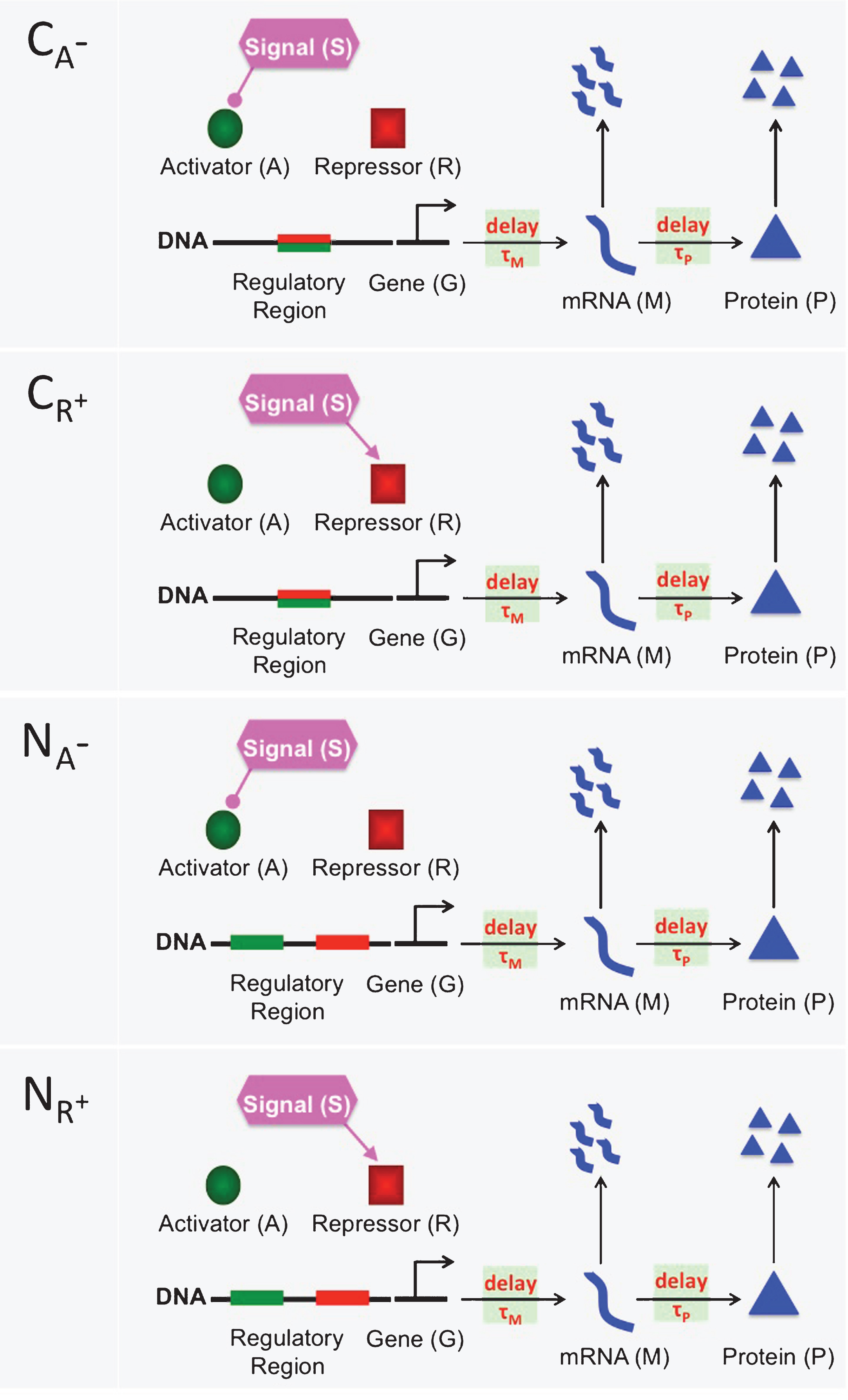
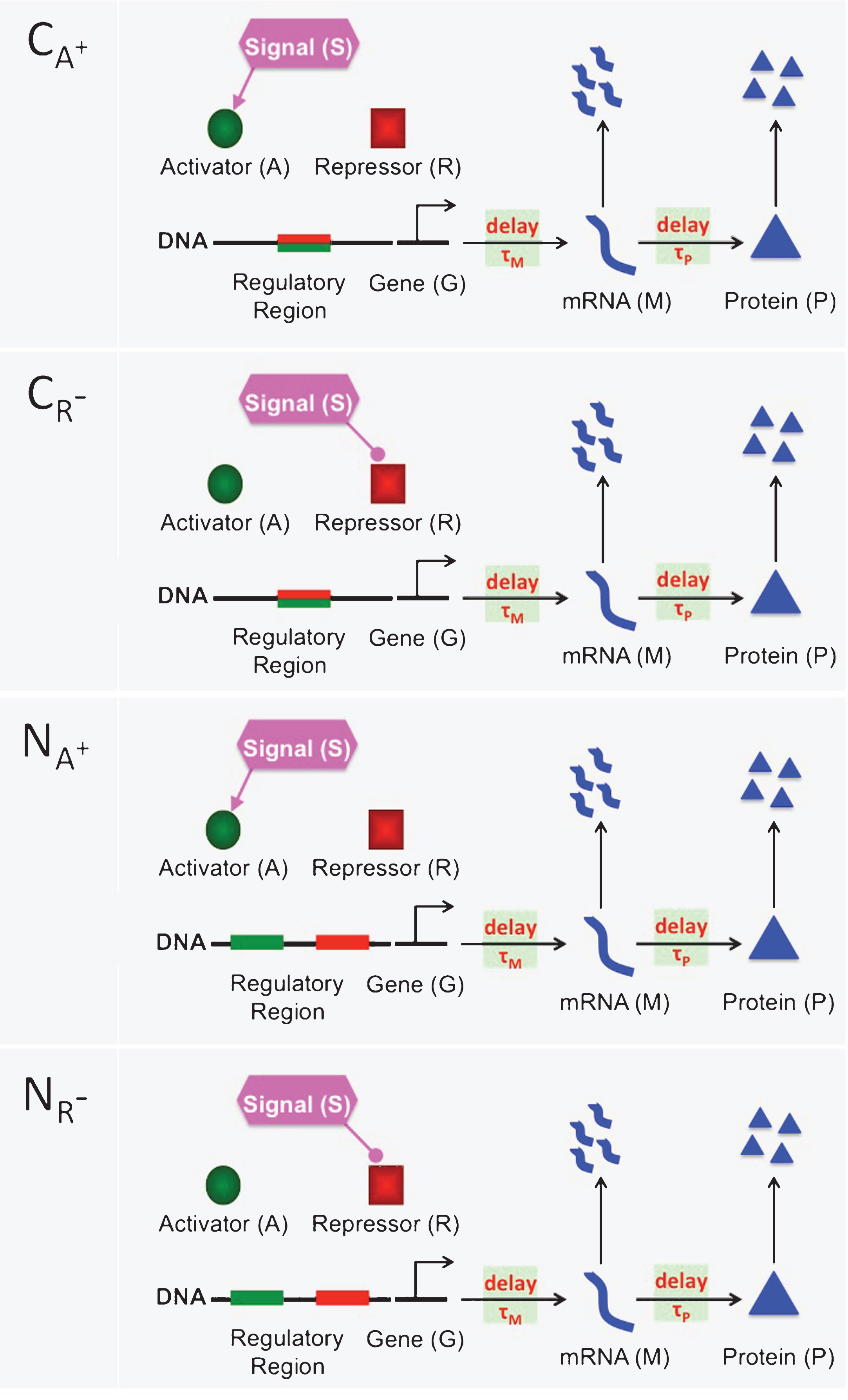
Fig.2
A cartoon showing four different activation mechanisms CA+, CR−, NA+ and NR−. In the competitive mechanisms (CA+ and CR−), the activator protein (green circle) and the repressor protein (red square) compete to bind to the same regulatory region(green-red rectangle) of DNA. In the noncompetitive mechanism (NA+ and NR−), there are two separate binding sites on the regulatory region, one is for the activator protein (green rectangle) and the other is for the repressor protein (red rectangle). In all figures, the lines coming out of the signal with rounded ends show a decrease in the activator and repressor abundance. Similarly, directed arrows represent an increase in the activator and repressor abundance. The horizontal arrows between gene (G) and mRNA (M) represent transcription process, which can be downregulated by the repressor protein and upregulated by the activator protein. The horizontal arrows between mRNA (M) and Protein (P) denote the translation of mRNA to protein. Finally, the vertical arrows represent degradation of mRNA and protein. Here, τM and τP are for the transcriptional and translational time delays, respectively.
We have utilized mass-action kinetics based on delay differential equation (DDE) models to study the dynamic responses produced by these regulatory mechanisms as a response to the transient signal. Through these mechanisms, a cell can increase or decrease the protein abundance through transcription by employing different regulatory interactions.
Some abbreviations are used in naming the mechanisms for the practical purposes. In a mechanism’s name, C stands for competitive binding and N stands for noncompetitive binding. The letters R and A respectively represent regulations through repression and activation. The sign + represents increase and - illustrates decrease in the levels of the regulatory proteins. More specifically, mechanism CR− is the mechanism activation in the competitive binding mechanism and activation is due to the decrease in the repressor protein levels, while mechanism NA− is the inhibition mechanism in the noncompetitive binding mechanism and inhibition is due to the decrease in the activator protein levels.
2.1Gene Regulation with Competition
In the competitive model, the net rate of change in repressor bound gene complex (
(1)
Similarly, the rate of change of activator bound gene levels (
(2)
Since we assume that the total gene abundance stays constant over time, the following equation holds
(3)
Hence, we only model the abundances of two states of the gene GR and GA.
The dynamics of mRNA abundance is described by Equation (4). We assume the rate of change in the mRNA abundance (
(4)
The dynamics of the protein P is modeled by Equation (5). We assume that the net rate of change in the protein abundance (
(5)
mRNA transcription from DNA and protein translation from mRNA are not instantaneous processes. RNA polymerase must traverse the gene and ribosomes should elongate through mRNA to translate it into protein. We included delay terms τm and τp in the different states of the gene and mRNA to account for the time it takes for the entire process to be completed. Here, for example, Gτm = G (t − τm), which represents the abundance of G not at time t, but at a time τm ago.
To explore the signal dependent responses of these simple regulatory mechanisms, we assume that the levels of the activator protein A and the repressor protein R in the models are regulated through a transient signal S (t), which is assumed to be a step function characterized by two positive parameters γ and k as in Equation (6)
(6)
Here the signal amplitude parameter (γ) measures the system’s sensitivity to the perturbation caused by the signal, and the signal persistency parameter (k) determines how long the signal is applied to the system. For example, to model a signal-induced repression in the competitive model, activator level A0 can either be decreased by the signal
2.1.1 The steady state analysis of competition models
The steady state analysis for the competition models have been performed. The details of the derivation can be found in Appendix. The steady state equation for the three states of the gene G, mRNA(M) and protein(P) are
(7)
(8)
(9)
(10)
(11)
2.2Gene Regulation Without Competition
The temporal evolution of the receptor-gene complex is modeled by Equation (12). It is assumed that the net rate of change in the repressor-gene complex (
(12)
The rate of change of activator bound gene (
(13)
(14)
(15)
(16)
2.1.2 The steady state analysis for the gene regulation without competition
The steady state analysis for the noncompetition models have been performed. The details of the derivation can be found in Appendix. The steady state equation for the four states of the gene G, mRNA(M) and protein(P) are
(17)
(18)
(19)
(20)
(21)
(22)
3Parameter values
In this section, the details of the parameter estimation or collection are given for E.coli cell.
• βm: The average mRNA half life is estimated as 5 - 10 minutes for E.coli [36]. In another study, the median mRNA half life has been measured to be 3.69 ± 0.49 [5]. We took 5 minutes for the mRNA half-life in this study. Assuming the degradation occurs exponentially, which gives an estimate of
• ηm0 and ηma: The average mRNA copy number per cell in E.coli shows variation, which is experimentally measured to be between 0.1 and 60 mRNA molecules per cell [35]. In another recent study, quantitative system wide measurements of mRNA and protein levels in individual cells using single-molecule counting technique have been used. This study showed that the average mRNA copy number per cell ranges from 10−3 to 10 [36]. In this study we took the steady state level of 4 mRNA molecules per cell. We assume that the transcription rate of the activator bound state GA is 10 times faster than that of the free state G, i.e. ηma = 10ηm0. From Equation (10), the steady state of mRNA is given by the equation
• αm0, αma and αmar: It is assumed that the transcription rate of the activator bound state GA and the activator and repressor bound state GAR are respectively 10 and 3 times faster than the transcription rate of the free state G. Hence, we have αma = 10αm0 and αmar = 3αm0. From Equation (21), the steady state of mRNA is given by the equation
• βp: The protein half-life changes from protein to protein and varies from 15 to 120 minutes in E.coli [41]. If the temporal degradation profile is exponential, then these figures give two estimates of 0.0462 and 0.0057 min−1 for βp. Here, we used βp = 0.02 min−1, which is approximately equal to the average of these two figures and provides a protein half-life of 35 minutes.
• αp: Molecular abundances of all proteins in E. coli have been experimentally studied by advanced proteomic technologies, and were classified into three groups [13]. In the same study, they reported that the protein numbers for E. coli range from ∼100 to 105. By Equation (11) and (22), we have αpM* = βpP*, which leads to an estimate of
• τm: The average mRNA length is measured to be 1000 nucleotides in E.coli [16]. RNA polymerase transcription rate of mRNA has been estimated as 39 − 55 nt/sec [6]. We took the rate 39 nt/sec, which corresponds to the smallest doubling rate 0.6 doubling per hour. This results in
• τp: The ribosomal elongation rate in E.coli varies between 12 to 33 amino acids per second [18, 23]. In another study, it has been reported that the translation rate is between 12 and 21 amino acids per second [6]. In the same study, they reported the translation rate as 12 amino acids per second for a bacteria with doubling rate of 0.6 doubling per hour. Here we use a generic protein with average mRNA length of 1000 nucleotides. Using this figure we obtain
4Results
We analyzed dynamics produced by the competitive and noncompetitive activatory and inhibitory binding mechanisms whose equations are listed in Table A.1 and Table A.2. All the simulations and analysis were implemented in Matlab using the biologically realistic estimates for the parameters detailed in Section 3. In the simulations, the signal persistency parameter k changes from 10 to 100 minutes, the signal amplitude parameter γ varies between 10-fold and 100-fold and ro parameter varies between 10−4 and 10−1, while all the others are held at their values listed in Section 3. We will focus on the discussion of the results for the binding constant ro = 10−4 here. The simulation results for ro = 10−3, ro = 10−2 and ro = 10−1 have been provided in the Appendix. Different mechanisms show comparable mP dynamics for varying ro levels. However, the differences between the mechanisms become negligible for mT and D metrics as this parameter increases.
4.1Inhibition mechanisms
In this section, we studied the competitive and noncompetitive inhibition mechanisms that result in a decrease in the protein abundance as a result of a transient signal. We denote the competitive binding mechanism in which the activator protein abundance is decreased by CA−. CR+ represents the competitive binding mechanism in which the repressor level is increased by a signal. On the other hand, the abbreviations NA− and NR+ stand for the noncompetitive mechanisms that a transient signal decreases the activator or increases the repressor levels, respectively.
4.1.1Comparison of the competitive inhibition mechanisms
The effects of the transient constant signal on the protein abundance in the competition models were studied. In these two mechanisms, the activator and repressor proteins compete for binding to the same regulatory site on DNA. The abbreviation CA- stands for the competitive mechanism in which the activator protein abundance is decreased by the signal. On the other hand, CR+ is the competitive mechanism in which the repression is due to an increase in the repressor protein abundance by the signal. In both mechanisms, the protein abundance decreases due to the signal.
The results of our simulations for the response metrics mP, mT and D are shown in Fig. 3 as γ values change between 10 and 100, and k varies from 10 to 100 minutes when ro = 10−4. Our simulations show different dynamics for the mid-protein mP levels of the mechanisms CA− and CR+. In CA− mechanism, mP remains approximately constant as the signal amplitude increases for the fixed signal persistency. However, when the signal amplitude is small (γ < ∼20) and the signal persistency is large (k > ∼60 min), mP shows slight nonlinear behavior. On the other hand, CR+ displays more nonlinear dependence on the signal, particularly for smaller γ values. For varying signal profiles, while mP changes between 82 molec./cell and 98 molec./cell in CA−, it varies from 74 molec./cell to 95 molec./cell in CR+. Each mechanism reaches the minimum mP levels when the signal persistency and signal amplitude are at their maximum, i.e. k = 100 min and γ = 100 fold.
Fig.3
Heat maps for the comparison of three metrics (mid-protein level mP, time to reach mid-protein level mT and duration D) describing the dynamics of competitive (CA−, CR+) and noncompetitive (NA−, NR+) inhibition mechanisms. In these simulations, the signal amplitude γ and persistency k range from a 10-fold to a 100-fold change when ro = 10−4. All the other parameters were held constant at their values listed in Section 3. See text for the details.
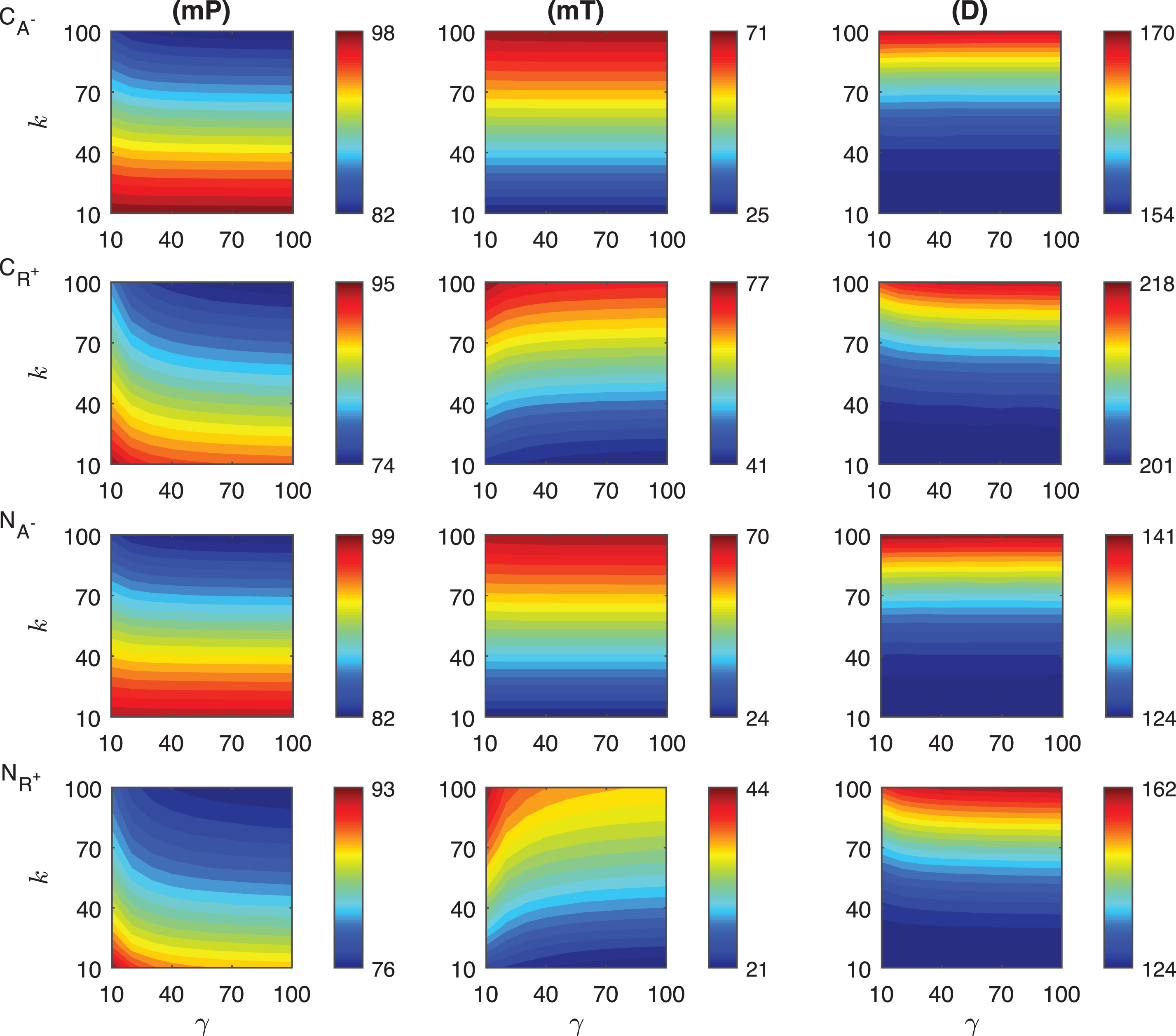
The heat maps for the mT levels have similar behavior for both of the competition mechanisms CA− and CR+. mT remains constant as the signal magnitude γ increases with fixed signal persistency k in CA− mechanism. CR+ mechanism displays nonlinear dependence to signal for smaller γ. Unlike what is observed in the mP metric, the variation in mT is larger in CA− than the values in CR+. While mT changes between 25 min and 71 min in CA−, it varies from 41 to 77 min in CR+. We observe that the time required to reach mP is significantly shorter (∼25 min) in the CA− than the values CR+ mechanism can produce (∼41 min).
The qualitative behavior of the duration metric D for both mechanisms is quite similar. For the signal with fixed persistency, D does not change as γ increases in CA−. For fixed γ levels, D increases with k. For a fixed value of γ, D increases as k increases nonlinearly for all values of γ in both mechanisms. However, this nonlinear behavior changes for different values of γ in the CR+ mechanism. The quantitative variation in the metric D is surprisingly similar for both mechanisms. While in CA−, the D changes between 154 min and 170 min, it varies from 201 min to 218 min. in CR+.
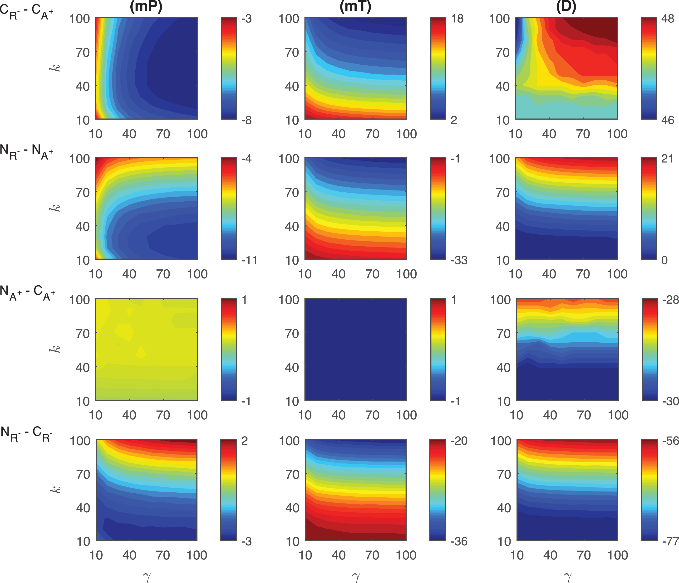
Differences in the competitive inhibition mechanisms: The results of our simulations for the differences of response metrics mP, mT and D are depicted in Fig. 4. mP level in CR+ is always ∼3 −8 molecules less than what has been observed in CA− for varying signal profiles. This difference is heavily dependent on the signal amplitude γ and gets larger as γ increases. For all the signal profiles considered, mT level in CA− is always ∼2 −18 minutes smaller than the values in CR+. This difference is more dependent on the signal persistency k and it gets larger as k increases. Our simulation also shows that the difference in mT is highest for shorter signal persistency (γ = 10) and amplitude (k = 10). The duration metric D is always bigger in CR+ than its value in CA−. For the varying signal profiles, D is ∼46 − 48 minutes longer in CR+. This difference takes its maximum value when both γ and k are relatively large, however it becomes smallest when k > ∼80 and γ < ∼15.
Fig.4
Heat maps for the comparison of the differences of three metrics (mid-protein level mP, time to reach mid-protein level mT and duration D) showing the dynamics of competitive (CA−, CR+) and noncompetitive (NA−, NR+) inhibition mechanisms. For all these simulations, the signal amplitude γ and persistency k are changed from 10-100 fold when ro = 10−4 while all the other parameters were kept constant at their estimated values listed in Section 3. For details see the text.
4.1.2Comparison of the noncompetitive inhibition mechanisms
We then examined the change of the protein abundance in the noncompetitive binding mechanisms for varying persistent signal profile. In these mechanisms, the activator and repressor proteins bind different regulatory regions of DNA. Here NA− represents the mechanism, in which the activator protein level is decreased by the signal. In the second mechanism(NR+), the repressor protein abundance is increased with the signal. The results of our simulations for the response metrics mP, mT and D are summarized in Fig. 3 for γ values changing between 10 and 100, and k values changing between 10 and 100 minutes when the parameter ro is 10−4.
The mid-protein levels mP for the two noncompetitive mechanisms have distinct dynamics as shown in the last two rows of Fig. 3. As the signal amplitude increases, mP does not change significantly for the fixed signal persistency in NA−. However, when the signal amplitude is small (γ < ∼20) and the persistency is large (k > ∼60 min), mP has nonlinear dependence on these parameters. In NR+ mechanism, mP dependence on the signal parameters is more nonlinear than what has been observed in NA− mechanism. The quantitative variation in mP is almost the same in both mechanisms, and changes from 82 molec./cell to 99 molec./cell in NA− and from 76 molec./cell to 93 molec./cell in NR+. The minimum mP abundance in each mechanism is reached when the signal profile has the maximum persistency (k = 100 min) and amplitude (γ = 100 fold).
The mT metric shows significantly different dynamics in these mechanisms. For the fixed signal persistency while this metric takes relatively constant values in NA− mechanism, it has a nonlinear dependence on the signal amplitude in NR+ mechanism. When the signal amplitude is small (γ < ∼20) and the signal persistency is large (k > ∼60 min), this nonlinearity increases in NR+ mechanism. The time variation is larger in NA− than in NR+, which is 46 minutes and 23 minutes, respectively. In both mechanisms, minimum values for the mT metric are comparable, NA− mechanism has its minimum at 24 min and NR+ mechanism’s minimum is at 21 min. mT changes from 24 min to 70 min in NA− and from 21 min to 44 min in NR+ mechanism.
Our simulations show that the duration metric D has similar qualitative performance in both mechanisms and the dependence of this metric on the signal is roughly linear. For fixed signal persistency, D remains constant as the signal amplitude varies. The slight nonlinearity is observed for smaller signal amplitude (γ < ∼15) with large persistency (k > ∼50 min) in NR+ mechanism. The quantitative change of D in NR+ mechanism is approximately twice as much as that of in NA−, which are 38 min and 17 min, respectively.
Differences in the noncompetitive inhibition mechanisms: The results of our simulations for the differences of response metrics mP, mT and D are depicted in the second row of Fig. 4. The difference in mid-protein levels between the two noncompetitive models is ∼4 −11 molecules for the range of signal profiles considered. mP metric takes lower values in NR+ than in NA−. The biggest difference is observed for large signal amplitude (γ > ∼70) with a small persistency (k < 30 min). NR+ mechanism has ∼1 −33 minutes shorter mT levels than NA−. The difference of mT between two mechanisms depend on the signal linearly as the signal persistency increases (γ > ∼30). The maximum difference is observed when the signal persistency and amplitude are at their maximum levels. The duration metrics D takes ∼0 −21 minutes longer in NR+ than in NA−. It remains approximately constant for large signal amplitude (γ > ∼20) for all signal persistency considered. It reaches its maximum value for the largest signal amplitude with the longest signal persistency.
4.1.3Comparison of the competitive and noncompetitive inhibition mechanisms for decreasing activator levels
We compared the change of the protein abundance in the competitive and noncompetitive binding mechanisms depending on varying signal profile. In the activator dependent inhibition mechanisms CA− and NA−, the activator protein abundance is decreased by the signal. CA− stands for the activator dependent competitive inhibition mechanism, and NA− represents the activator dependent noncompetitive inhibition mechanism. The results of our simulations for the response metrics mP, mT and D are shown in first and third rows in Fig. 3 while the parameters γ and k changes between 10 and 100 and when ro = 10−4. The mid-protein mP levels of the competitive and noncompetitive binding mechanisms have a relatively similar dynamics as shown in the first and third rows of Fig. 3. Our simulations predicts that for fixed signal persistency levels the mP levels do not show significant change in both mechanisms. However, if the signal amplitude γ is held constant, the mP levels decrease in a linear fashion as signal persistency increases. In both mechanisms when the signal amplitude is small (γ < ∼10) and the signal persistency is large (k > ∼60 min), mP depends on the signal in a nonlinear fashion. The quantitative variation in mP is roughly the same in both mechanisms for all the signal profiles considered. mP level changes from 82 molec./cell to 98 molec./cell in CA− and from 82 molec./cell to 99 molec./cell in NA−. The minimum mP abundance for each mechanism are reached when the signal profile has the maximum persistency (k = 100 min) and amplitude (γ = 100 fold).
In both mechanisms mT levels show similar dynamics for varying signal profile. As the signal persistency gets longer, the mT values increases linearly in the both mechanisms. However, if the signal persistency is held fixed, mT does not change as the signal amplitude increases. The quantitative change in mT is 46 minutes for both CA− and NA−. Both mechanisms require roughly the same time to reach mid-protein abundance. While mT changes from 25 min to 71 min in CA− mechanism and from 24 min to 70 min in NA− mechanism.
The duration metric D has similar qualitative performance. For fixed signal persistency k, D remains constant as the signal amplitude varies. However, for a fixed signal amplitude, our simulations predict a non-linear increase of D as the signal persistency k gets longer. The quantitative variation of D in both mechanisms are also different, It is 16 min in CA− and 17 min in NA−. D changes from 154 min to 170 min in CA− and from 124 min to 141 min in NA− mechanism.
Differences in the competitive and noncompetitive inhibition mechanisms for decreasing activator levels: The differences of response metrics mP, mT and D are depicted in the third row of Fig. 4. The mP abundance difference between the mechanisms is negligible for all the signal profiles. Our simulations predict that there is no significant difference in mT metric for varying signal profiles. However, our simulations show that the duration metric D is ∼28 − 30 minutes longer in CA− than the duration in NA−. The difference in metric D takes on its minimum for signal persistency k > ∼75 minutes and attains its longest value when k < ∼25minutes.
4.1.4Comparison of the competitive and noncompetitive inhibition mechanisms for increasing repressor levels
Lastly, we compared the effect of the transient constant signal on the protein abundance in the competitive and noncompetitive binding mechanisms for increasing repressor levels. As a reminder, CR+ and NR+ stand for the competitive and noncompetitive mechanisms respectively in which the repressor protein abundance is increased by the transient signal. In both mechanisms, the protein abundance decreases due to signal. The response metrics mP, mT and D are shown in Fig. 3 for γ values in between 10 and 100 folds, and k changes between 10 and 100 minutes when ro = 10−4.
Our simulations show that both models have similar mid-protein mP levels. When the signal amplitude is large (γ > ∼50), mP remains approximately constant as the signal amplitude increases for the fixed signal persistency in both mechanisms. However, when the signal amplitude is small (γ < ∼50), mP has nonlinear behavior. Moreover, mP changes between 74 molec./cell and 95 molec./cell in CR+ and it varies from 76 molec./cell to 93 molec./cell in NR+.
mT behaves nonlinearly in both mechanisms when the signal amplitude is less than 50 and linearly otherwise. They both reach their maximum values for the smallest signal amplitude and the largest persistency. We observe the difference of their quantitative variations are at the extreme values. The quantitative difference in CR+ mechanism is approximately 1.5 fold more than what it is in NR+, which are 36 molec./cell and 23 molec./cell, respectively. mT changes between 41 molec./cell and 77 molec./cell in CR+, it varies from 21 molec./cell to 44 molec./cell in NR+.
The dependence on the signal of the duration metric D is nonlinear for both mechanisms when the signal amplitude is small (γ < ∼20). The quantitative variation in the metric is quite different between the two mechanisms. While in CR+, the D changes between 201 min and 218 min, in NR+, it varies from 124 min to 162 min and the difference in NR+ mechanism is twice as much as what it is in CR+ (17 min vs 38 min).
Differences in the competitive and noncompetitive inhibition mechanisms for increasing repressor levels: The differences of response metrics mP, mT and D are depicted in Fig. 4. For smaller persistency (k < ∼50), mP level in CR+ is bigger than in NR+. When the signal persistency and amplitude approach to their maximum values, the opposite happens. Moreover, a nonlinear relation is observed in the heat map for smaller γ amplitudes (γ < ∼20). For all the signal profiles that we have considered, mT level in CR+ is always ∼20 − 36 minutes bigger than what is observed in NR+. This difference is more dependent on the signal persistency k and it gets bigger as k increases. The duration metric D is always bigger in CR+ than in NR+. D is ∼56 − 77 minutes longer in CR+ for the varying signal profiles. This difference takes its maximum value when k has smaller values.
4.2Activation mechanisms
In this section, we studied the competitive and noncompetitive activation mechanisms that result in an increase in the protein abundance as a result of a transient signal. We denote the competitive binding mechanism in which the activator protein abundance is increased by CA+. CR− represents the competitive binding mechanism in which the repressor level is decreased by a signal. On the other hand, the abbreviations NA+ and NR− stand for the noncompetitive mechanisms that a transient signal increases the activator or decreases the repressor levels, respectively.
4.2.1Comparison of the competitive activation mechanisms
In the competitive activation mechanisms, we assume the transient signal increases the activator or decreases the repressor level which leads to an increase in protein P abundance. In these mechanisms, the activator and repressor proteins compete to bind the same regulatory site on DNA thereby regulating the synthesis rate of the mRNA for the protein P. The heat maps of the response metrics mP, mT and D are depicted in Fig. 5 for these two mechanisms where the signal amplitude, γ, changes between 10 and 100 fold, and the signal persistency, k, varies from 10 to 100 minutes when the binding rate constant ro is held constant at 10−4.
Fig.5
Heat maps for the comparison of three metrics (mid-protein level mP, time to reach mid-protein level mT and duration D) describing the dynamics of competitive (CA+, CR−) and noncompetitive (NA+, NR−) activation mechanisms. In these simulations, the signal amplitude γ and persistency k range from 10-fold to 100-fold change when ro = 10−4. All the other parameters were held constant at their values listed in Section 3. See text for details.
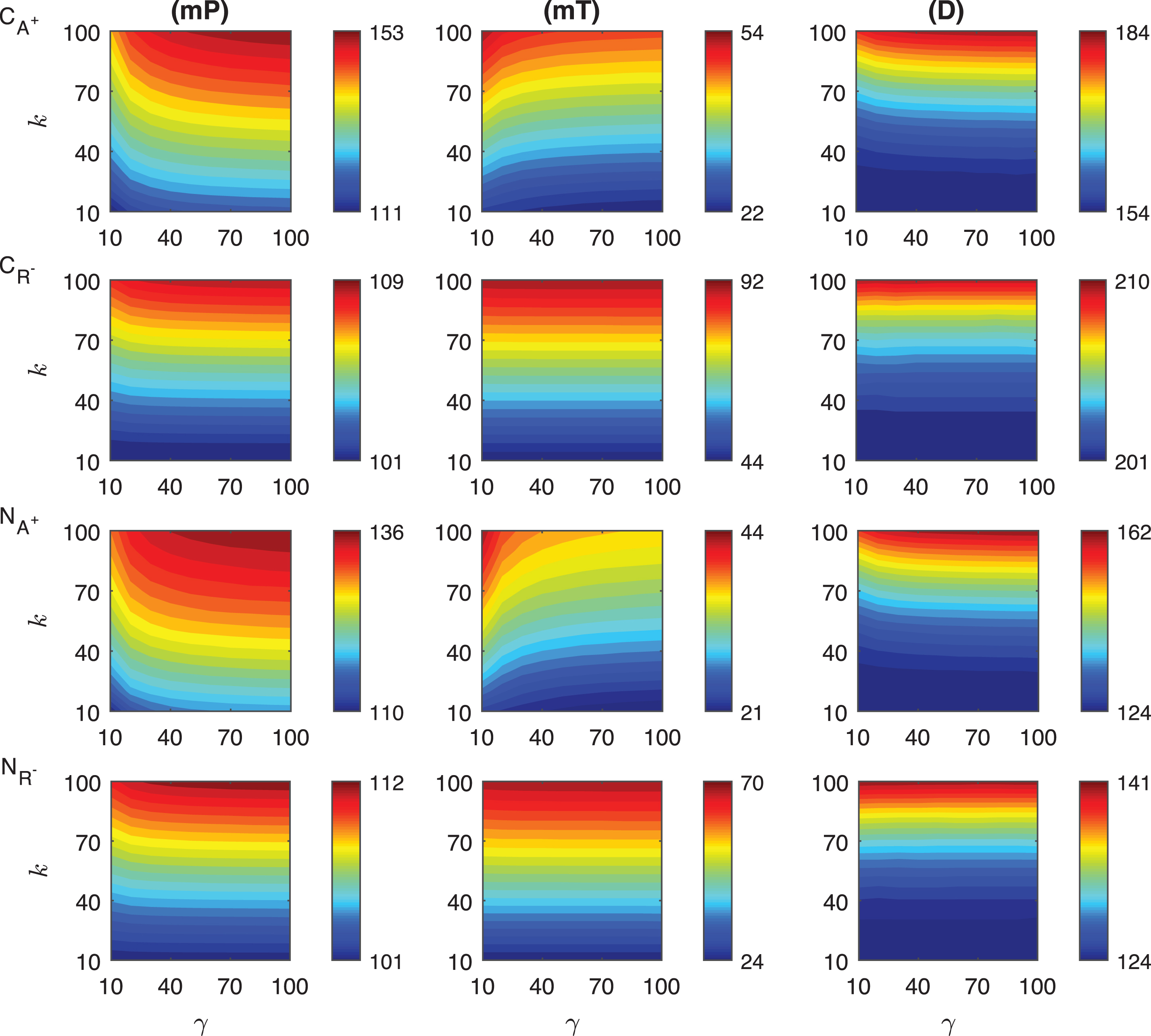
The change in the mid-protein levels for CA+ and CR− mechanisms show different quantitative and qualitative dynamics as shown in the first two rows of Fig. 5. The dependence on the signal is nonlinear in CA+ mechanism, while it is almost linear in CR−. This linearity is more noticeable for the higher signal amplitude (γ > ∼20). In both mechanisms, the highest mP values are attained when the signal amplitude and persistency are at their maximum values, i.e. γ = 100 fold and k = 100 minutes. It is obvious from our simulations that increasing activator protein results in more increase in mid-protein abundance, mP. In CA+ mechanism, mP changes from 111 molec./cell to 153 molec./cell. On the other hand, in CR− mechanism, it varies only between 101 molec./cell and 109 molec./cell.
The mT metric shows slightly different dependence on the transient signal for each mechanism. In CR−, mT remains constant for the fixed signal persistency and increasing signal amplitude. However, in CA+ mechanism, it has nonlinear dependence on the signal for smaller signal amplitudes (γ < 30). mT is in average shorter in CA+ mechanism than in CR−. mT level ranges between 22 and 54 min in CA+ while it ranges from 44 to 92 min in CR−.
The duration metric D varies quite nonlinearly for large signal persistency (k > ∼60 min) in CA+ mechanism, while its dependence on the signal is more linear in CR−. For fixed signal persistency levels, D does not change significantly in CR− as signal amplitude increases. Quantitatively, D metric changes from 154 to 184 minutes in CA+ and from 201 to 210 minutes in CR−. We can conclude that CR− mechanism stays above the mid-protein level longer thanCA+.
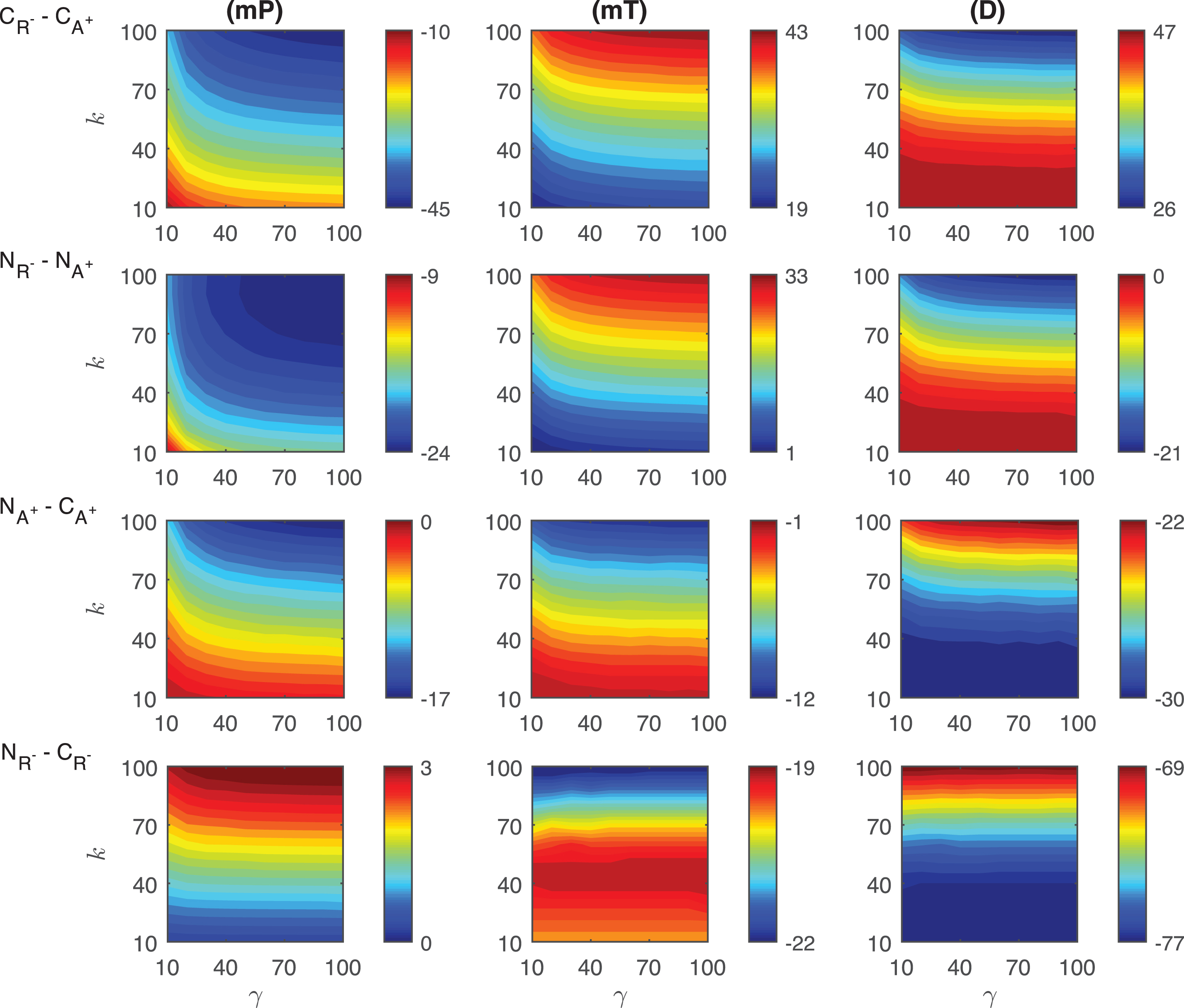
Differences in the competitive activation mechanisms: The differences of the response metrics mP, mT and D are plotted in the first row of Fig. 6. The difference of mP levels depends on the transient signal nonlinearly. CA+ mechanism has ∼10 − 45 molecules more than CR−. As the signal amplitude and persistency increase, the difference also increases, and takes its maximum (∼45 molec./cell) at k = 100 and γ = 100. The difference of mT levels between two mechanisms changes nonlinearly and it increases as the signal persistency increases. CR− mechanism always needs longer time to reach the highest protein level than CA+. The time difference between two mechanisms varies from ∼19 to ∼43 minutes. The maximum difference is observed when the signal amplitude and persistency reach their maximums. The difference between the duration metric D of two mechanisms produces nonlinear results for small signal amplitude (γ < 40 min). As the signal profile changes, CR− mechanism has ∼26 − 47 minutes more than CA+. The smallest difference is reached when k > 80, while the highest difference is observed when k < 20.
Fig.6
Heat maps for the comparison of the differences of three metrics (mid-protein level mP, time to reach mid-protein level mT and duration D) showing the dynamics of competitive (CA+, CR−) and noncompetitive (NA+, NR−) activation mechanisms. For all these simulations, the signal amplitude γ and persistency k are changed from 10-100 fold when ro = 10−4 while all the other parameters were kept constant at their estimated values listed in Section 3. For details see the text.
4.2.2Comparison of the noncompetitive activation mechanisms
We explored the effect of the signal on the protein abundance in the noncompetitive activation mechanisms in which the activator (NA+) and repressor (NR−) proteins bind different DNA sites, thereby both mechanisms lead to an increase in the protein abundance. The heat maps of the response metrics mP, mT and D are plotted in Fig. 5. The signal amplitude γ changes between 10 and 100 fold, and the signal persistency, k, alters from 10 to 100 minutes with the constant ro = 10−4.
Our simulations show that the mid-protein metric mP for each mechanism have different dynamics for varying signal profile. NA+ shows more nonlinear dependence on the signal amplitude, while NR− remains almost constant as the signal amplitude increases for the fixed signal persistency. We observe that, NR− has a slight nonlinearity when k > ∼60 minutes and γ < ∼20. Quantitatively, the metric mP in NA+ mechanism varies from 110 molec./cell to 136 molec./cell, and while it changes from 101 molec./cell to 112 molec./cell in NR−.
The mT metric displays significantly different dynamics in both mechanisms. For all signal profiles, mT changes in a nonlinear fashion in NA+ mechanism, whereas it shows almost linear behavior in NR−. However, the highest mT level is observed when the signal persistency is at the maximum (k ∼ 100 min) for all signal amplitudes in NR− mechanism. The values of mT metric are also different in both mechanisms. mT changes from 21 to 44 minutes in NA+ and from 24 to 70 minutes in NR−. Overall, mT is shorter in NA+ than in NR−.
The duration metric, D, shows a comparable qualitative behaviour for varying signal profile. In NA+ mechanism, D has slight nonlinear dependence on the signal. In particular, for the small signal amplitude (γ < ∼20) and the large signal persistency (k > ∼60 min) the nonlinearity is more significant. On the other hand, in NR−, D stays unchanged as the signal amplitude varies for the fixed persistency. Although the smallest D values are the same for each mechanism, which is 124 min, the largest values are different, which is 162 min in NA+ and is 141 min in NR−.
Differences in the noncompetitive activation mechanisms: The differences of the response metrics mP, mT and D are displayed in the second row of Fig. 6. The mid-protein metric mP has ∼9 −24 molecules per cell smaller in NR− than in NA+. The maximum difference is observed for the largest signal amplitude and persistency. The difference changes nonlinearly with various signal profiles. For all signal profiles, the mT metric in NR− mechanism is larger than NA+. The difference of mT between two mechanisms is significantly nonlinear when the signal amplitude is small (γ < ∼30). Quantitatively, the time difference between two mechanisms is ∼1 −33 minutes. The maximum difference is reached when the signal amplitude and persistency are at their maximum. The duration metric D in NA+ mechanism is ∼0 −21 minutes more than in NR−. The greatest difference is obtained for the largest signal amplitude and persistency.
4.2.3Comparison of the competitive and noncompetitive activation mechanisms for increasing activator levels
We investigated the difference between the competitive and noncompetitive activation mechanisms as the activator protein levels increase. mP levels have very similar qualitative dynamics for both mechanisms, but distinct quantitative behavior. mP in CA+ changes from 111 molec./cell to 153 molec./cell and in NA+, from 110 molec./cell to 136 molec./cell. As signal varies, the metric mT shows slightly different qualitative and quantitative dynamics in both mechanisms. The maximum mT is 54 minutes in CA+ and 44 minutes in NA+. The minimum mT is 22 minutes in CA+ and 21 minutes in NA+. The duration metric D shows qualitatively similar, but quantitatively different dynamics. D changes between 154 and 184 minutes in the competitive mechanism, it varies from 124 to 162 minutes in the noncompetitive mechanism.
Differences in the competitive and noncompetitive activation mechanisms for increasing activator levels: We measured the differences of the response metrics mP, mT and D in the competitive and noncompetitive activation mechanisms, and the results are shown in the third row of Fig. 6. The difference between the mid-protein levels changes slightly nonlinearly for varying signal profile. NA+ mechanism has 0 − 17 molec./cell less than CA+.The difference in mT levels has a nonlinear dynamic as the transient signal varies. NA+ requires ∼1 −12 minutes less than CA+ to attain the mid-protein level. For all signal profiles, D metric of NA+ is ∼22 − 30 min less than that of CA+. The difference depends nonlinearly on the signal profile for smaller values of k.
4.2.4Comparison of the competitive and noncompetitive activation mechanisms via decreased repressor abundance
We investigated the difference between the competitive and noncompetitive activation mechanisms as the repressor protein abundance decreases.
Our simulations illustrate that both mechanisms have similar qualitative and quantitative dynamics in terms of mP. In CR− mechanism the mid-protein level starts at 101 molec./cell and goes up to 109 molec./cell. On the other hand, in the noncompetitive binding mechanism, NR−, the highest protein abundance is 112 molec./cell and its lowest is 101 molec./cell. Our simulations predict that mT levels are determined by k but not γ, and show qualitatively similar, but quantitatively distinct dynamics. For both mechanisms, the smallest values (24 and 44) are observed when k ∼ 10; and the largest mT levels (70 and 92) are attained when k ∼ 100. The duration metric D is mainly determined by k, and shows qualitatively similar, but quantitatively different dynamics. In both mechanisms, the smallest values (124 and 201) are observed when k ∼ 10; and the largest D levels (141 and 210) are attained when k ∼ 100.
Differences in the competitive and noncompetitive activation mechanisms via decreased repressor abundance: The differences in the competitive and noncompetitive activation mechanisms for decreasing repressor protein abundance are summarized in the last row of Fig. 6. The difference of mP levels varies nonlinearly as the transient signal differs, but quantitatively shows negligible difference (∼0 −3 molec./cell). As the signal persistency k increases, the mT difference between the two mechanism becomes larger. NR− needs ∼19 − 22 minutes less than CR−. The duration metric D in CR− is ∼69 − 77 minutes longer than in NR−. While D is dependent on signal persistency k nonlinearly, it is not affected by the changes in signal amplitude γ for fixed k levels.
5Discussions
One of the fascinating questions of biology is how to control the development and physiology of organisms. The answer of this question is encoded in the regulatory binding sites in the enhancer regions of genes. Understanding transcriptional regulation is essential for the analysis of cellular functions, disease mechanisms and evolutionary dynamics[9, 17, 40].
The binding sites in the enhancer region control the development and physiology of organisms by regulating both temporal and spatial expression of genes [7]. The arrangement of binding sites within the enhancer regions is critical to achieve proper biological function [22]. Mutations that affect the individual binding sites and their arrangements often lead to diseases and phenotypic diversity within and between species.
Mathematical models offer an alternative approach to biological experimentation for studying gene regulation. In this study, we explored competitive and noncompetitive binding site arrangements of an activator and a repressor protein, and examined inhibitory and activatory gene regulation dynamics. In the competitive mechanisms, the activator and repressor proteins compete to bind to the same regulatory DNA site, while they bind different regions of DNA in the noncompetitive mechanisms. In all mechanisms, the transient signal leads to an increase or decrease in the activator or repressor protein abundances resulting in a change in the gene expression.
Competitive and noncompetitive binding mechanisms have been shown to be important for many prokaryotic and eukaryotic organisms [9, 37]. Just to mention a few examples, in lac operon of E.coli, the repressor protein and RNA polymerase compete to bind to the same regulatory region of the structural genes of LacZ, LacY and LacA. When allolactose binds to the repressor protein, it can no longer bind to the regulatory region and RNA polymerase starts transcription, which leads to 1000-fold increase in the basal level of the genes’ products [25]. In early development of Drosophila melanogaster embryos, dorsal-ventral pattern formation is controlled through both competitive and noncompetitive binding [43]. In this system, Snail repressor protein competes to bind to the same regulatory site with Twist activator protein. However, the Snail protein represses the Dorsal activator in a noncompetitive fashion. Similarly, in the circadian clock network there is a competitive (but not noncompetitive) binding of Ror and Rev-Erb to the Bmal1 gene. One suggested difference between competitive and noncompetitive binding mechanisms is that these two mechanisms are capable of producing different qualitative dynamics in biological systems. In a recent study, Munteanu et al. has shown that competitive binding reduces the parameter space that leads to oscillations [24].
This study provides insights on the dynamics of the competitive and noncompetitive binding mechanisms by providing a comprehensive comparison. Our analysis suggests that the competitive and noncompetitive inhibition mechanisms exhibit comparable repression effectiveness, but the response time is the fastest in the noncompetitive inhibition mechanism through increased repressor abundance and the slowest in the competitive inhibition mechanism through increased repressor level. Although the four inhibition mechanisms all decrease protein levels, cells selectively use these regulatory mechanisms as needed. The systems that require an urgent response would be better off using the noncompetitive inhibition mechanism through increased repressor abundance. The competitive inhibition mechanism through increased repressor level might be better for the systems that need long-term responses or whose effects need not be immediate after the signal.
Similarly, our simulations show that the competitive and noncompetitive activation mechanisms by increased activator protein level display more effective and faster response in comparison to the competitive and noncompetitive activation mechanisms due to decreased repressor abundance. The biological systems that require urgent and severe response should make use of competitive and noncompetitive activation mechanisms by increased activator protein level. These observations can be tested experimentally using synthetically engineered genetic circuits utilizing fluorescent proteins. Our analysis emphasizes the importance of mathematical modeling for better understanding the gene regulation dynamics, which is the key for the analysis of cellular functions, disease mechanisms and evolutionary dynamics. Such knowledge is also important for finding better disease diagnoses and therapies.
We have to mention that the mathematical models used here are strictly deterministic in nature and based on the explicit assumption that one is dealing with a population of cells and large molecule numbers so that the law of large numbers is applicable. It is worth stressing that if one is interested in the details of the dynamics at the level of a single cell, a different approach has to be taken for the small number of molecules. Gillespie [11] has considered in detail how simulations of such situations could be performed and used by many others [17, 19, 21, 39, 42].
Author Contributions
N.Y. and A.A. designed the project and built the mathematical model. M.E.A. and E.A. wrote the codes and performed the computational simulations. N.Y., A.A. M.E.A. and S.N.O. analyzed simulation results. N.Y., A.A., M.E.A. and S.N.O. wrote the manuscript.
Acknowledgment
We thank members of the Ay and Yildirim laboratories for their comments. This work was partially supported by Colgate University Research Council Grant to Prof. Ahmet Ay and the New College of Florida Faculty Development Fund to Prof. Necmettin Yildirim.
Appendices
A. Appendix: mathematical models of gene regulation
A. 1.1Steady state analysis of the competition models
At the steady state, the following equations must hold:
(A.1)
(A.2)
(A.3)
(A.4)
(A.5)
(A.6)
(A.7)
(A.8)
A.1.2.Steady state analysis of the competition models
The steady state of this system can be computed by setting all the time derivatives to zero. That is
(A.9)
(A.10)
(A.11)
(A.12)
(A.13)
(A.14)
(A.15)
(A.16)
(A.17)
(A.18)
(A.19)
(A.20)
(A.21)
(A.22)
(A.23)
(A.24)
A.1.3Heat maps for the response metrics for the competitive and noncompetitive binding mechanisms
Repression Figures
Fig.A.1
Heat maps for the comparison of three metrics (mid-protein level mP, time to reach mid-protein level mT and duration D) describing the dynamics of competitive (CA−, CR+) and noncompetitive (NA−, NR+) inhibition mechanisms. In these simulations, the signal amplitude γ and persistency k range from a 10-fold to a 100-fold change when ro = 0.001. All the other parameters were held constant at their values listed in Section 3.
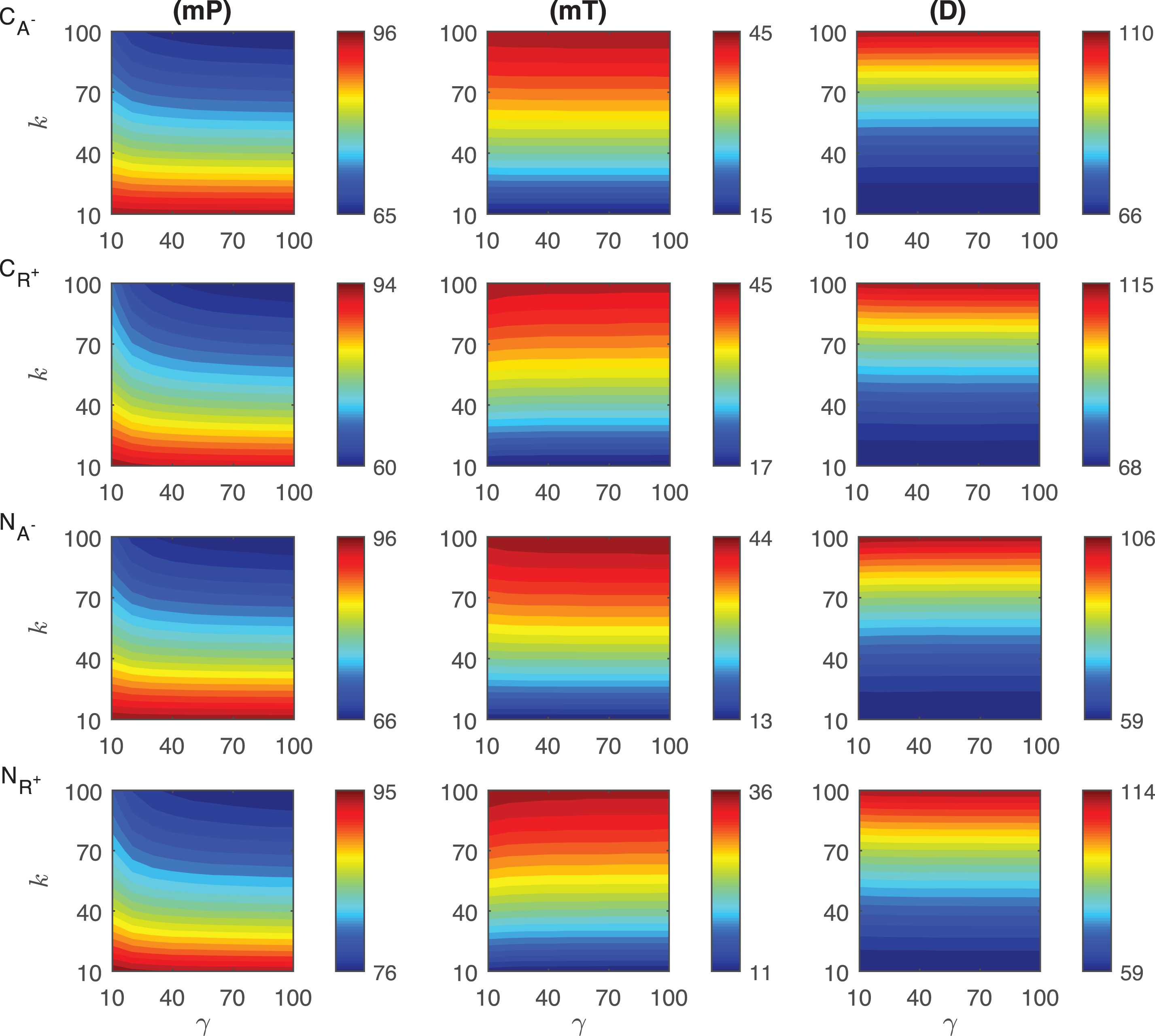
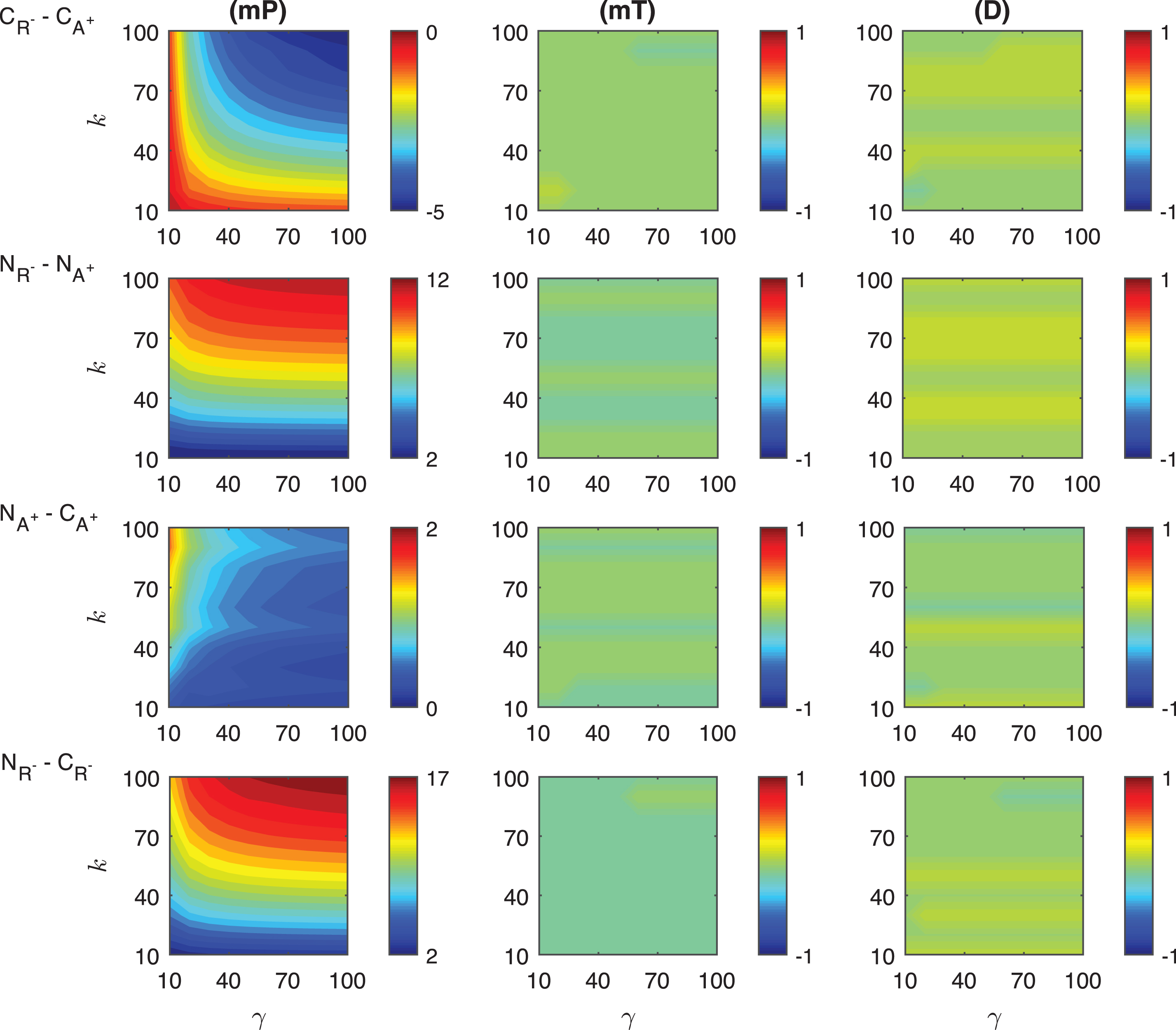
Fig.A.2
Heat maps for the comparison of the differences of three metrics (mid-protein level mP, time to reach mid-protein level mT and duration D) showing the dynamics of competitive (CA−, CR+) and noncompetitive (NA−, NR+) inhibition mechanisms. For all these simulations, the signal amplitude γ and persistency k are changed from 10-100 fold when ro = 0.001 while all the other parameters were kept constant at their estimated values listed in Section 3.
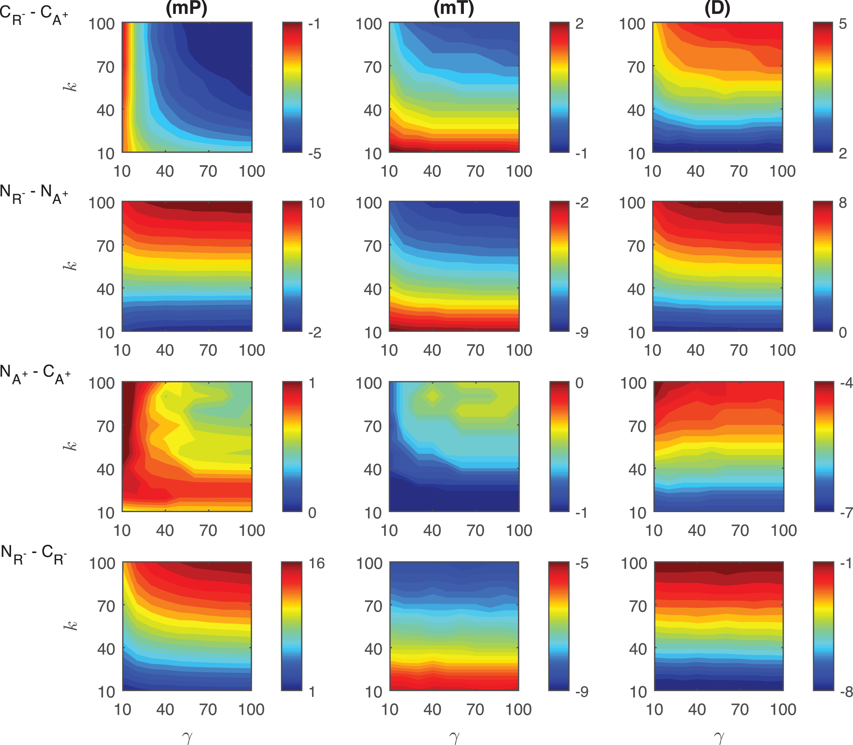
Fig.A.3
Heat maps for the comparison of three metrics (mid-protein level mP, time to reach mid-protein level mT and duration D) describing the dynamics of competitive (CA−, CR+) and noncompetitive (NA−, NR+) inhibition mechanisms. In these simulations, the signal amplitude γ and persistency k range from a 10-fold to a 100-fold change when ro = 0.01. All the other parameters were held constant at their values listed in Section 3.
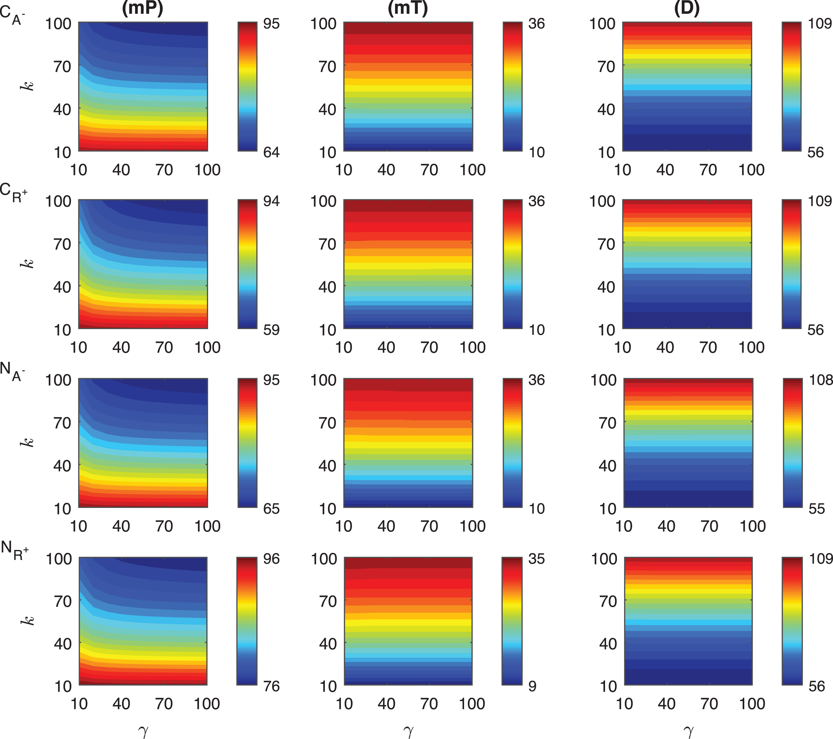
Fig.A.4
Heat maps for the comparison of the differences of three metrics (mid-protein level mP, time to reach mid-protein level mT and duration D) showing the dynamics of competitive (CA−, CR+) and noncompetitive (NA−, NR+) inhibition mechanisms. For all these simulations, the signal amplitude γ and persistency k are changed from 10-100 fold when ro = 0.01 while all the other parameters were kept constant at their estimated values listed in Section 3.
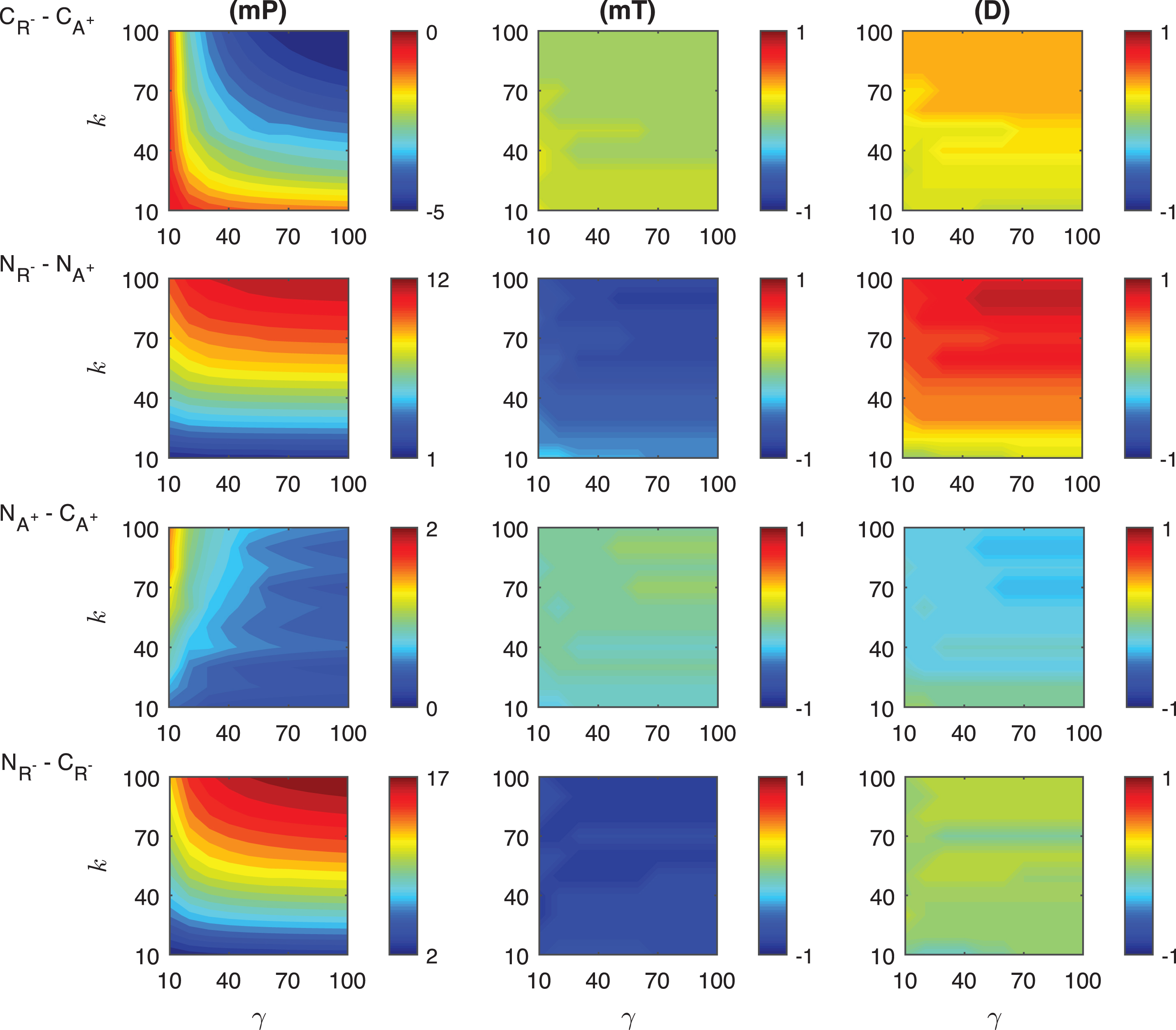
Fig.A.5
Heat maps for the comparison of three metrics (mid-protein level mP, time to reach mid-protein level mT and duration D) describing the dynamics of competitive (CA−, CR+) and noncompetitive (NA−, NR+) inhibition mechanisms. In these simulations, the signal amplitude γ and persistency k range from a 10-fold to a 100-fold change when ro = 0.1. All the other parameters were held constant at their values listed in Section 3.
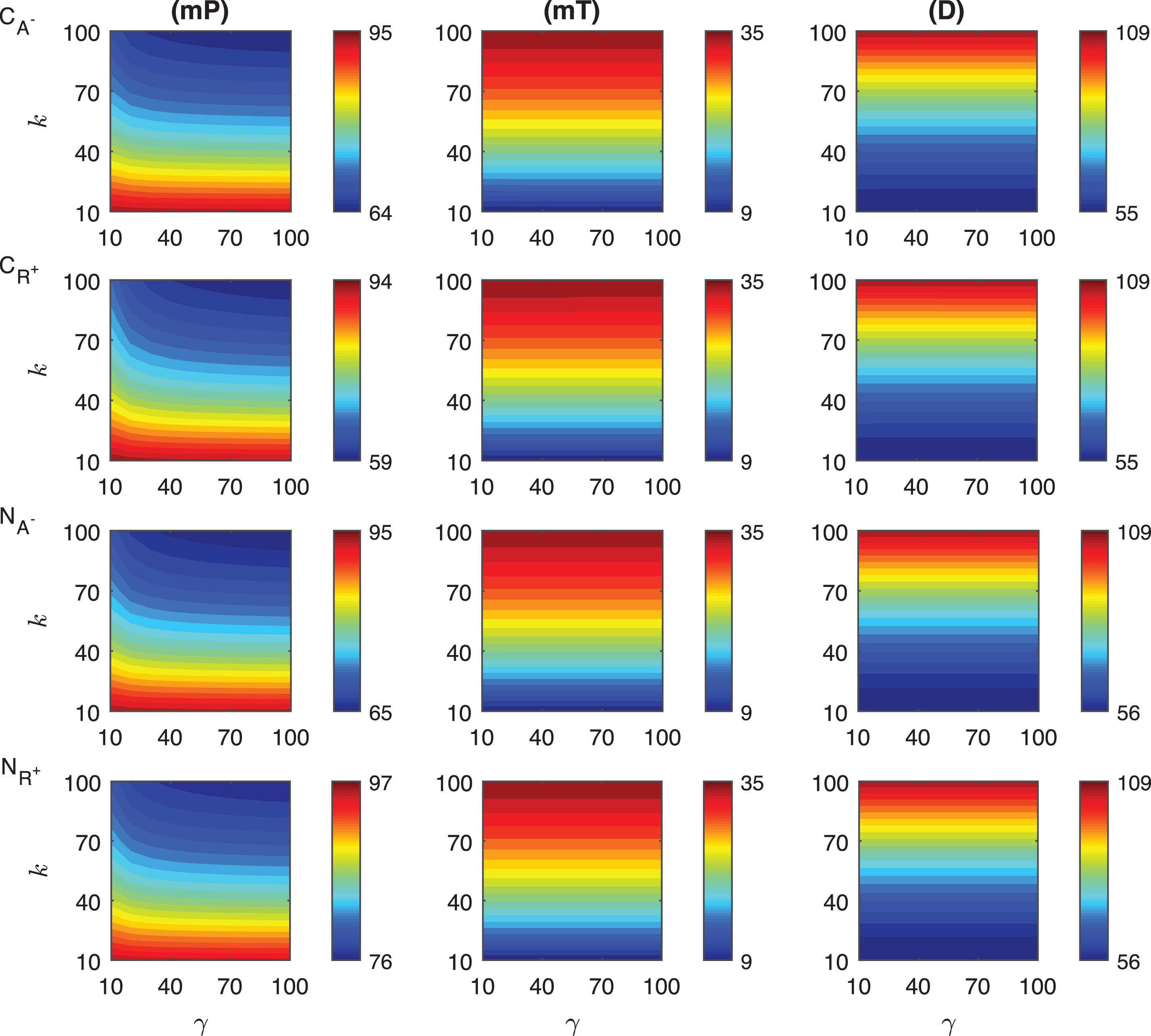
Fig.A.6
Heat maps for the comparison of the differences of three metrics (mid-protein level mP, time to reach mid-protein level mT and duration D) showing the dynamics of competitive (CA−, CR+) and noncompetitive (NA−, NR+) inhibition mechanisms. For all these simulations, the signal amplitude γ and persistency k are changed from 10-100 fold when ro = 0.1 while all the other parameters were kept constant at their estimated values listed in Section 3.
Activation Figures
Fig.A.7
Heat maps for the comparison of three metrics (mid-protein level mP, time to reach mid-protein level mT and duration D) describing the dynamics of competitive (CA+, CR−) and noncompetitive (NA+, NR−) activation mechanisms. In these simulations, the signal amplitude γ and persistency k range from a 10-fold to a 100-fold change when ro = 0.001. All the other parameters were held constant at their values listed in Section 3.
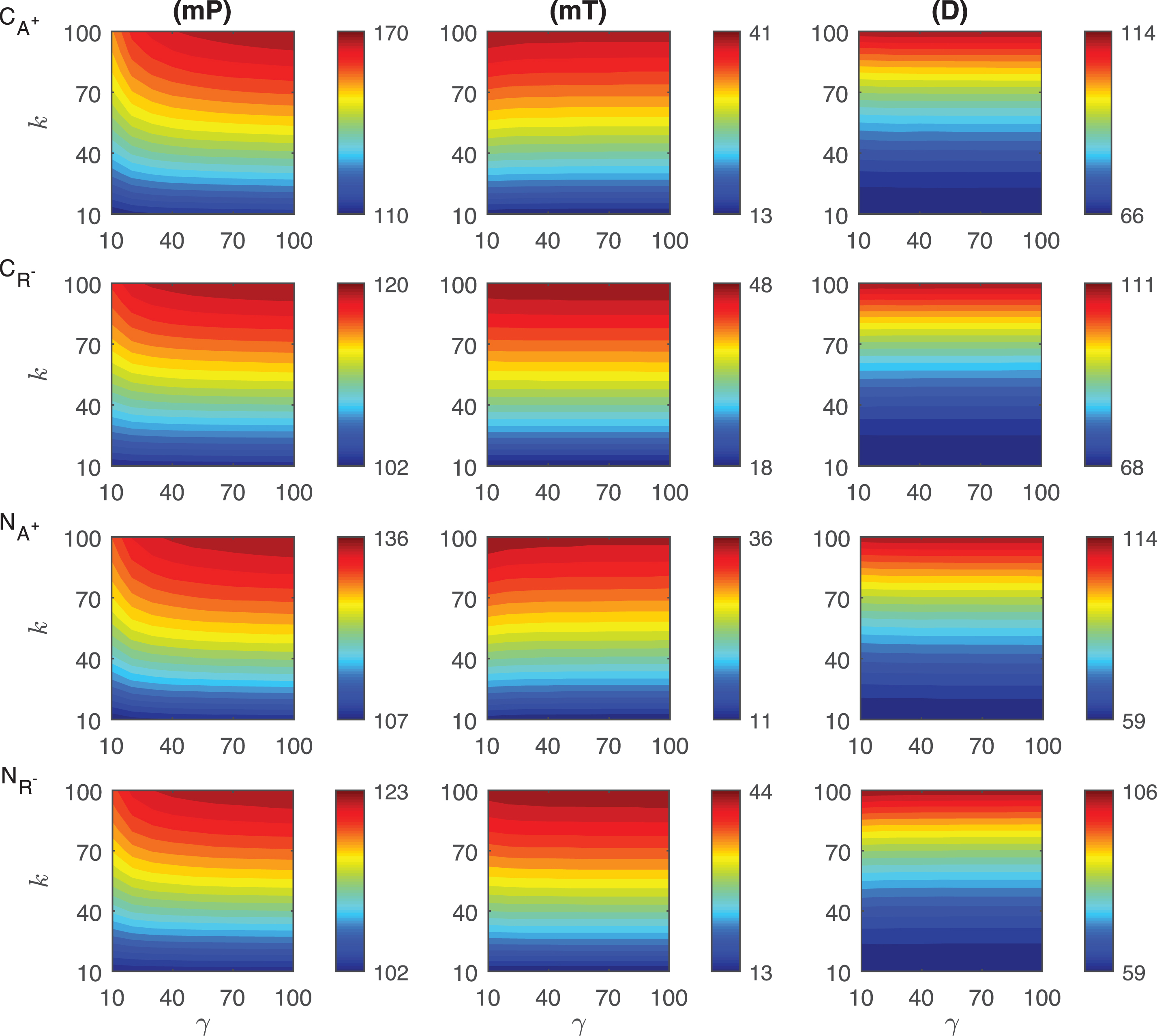
Fig.A.8
Activation Figures
Heat maps for the comparison of the differences of three metrics (mid-protein level mP, time to reach mid-protein level mT and duration D) showing the dynamics of competitive (CA+, CR−) and noncompetitive (NA+, NR−) activation mechanisms. For all these simulations, the signal amplitude γ and persistency k are changed from 10-100 fold when ro = 0.001 while all the other parameters were kept constant at their estimated values listed in Section 3.
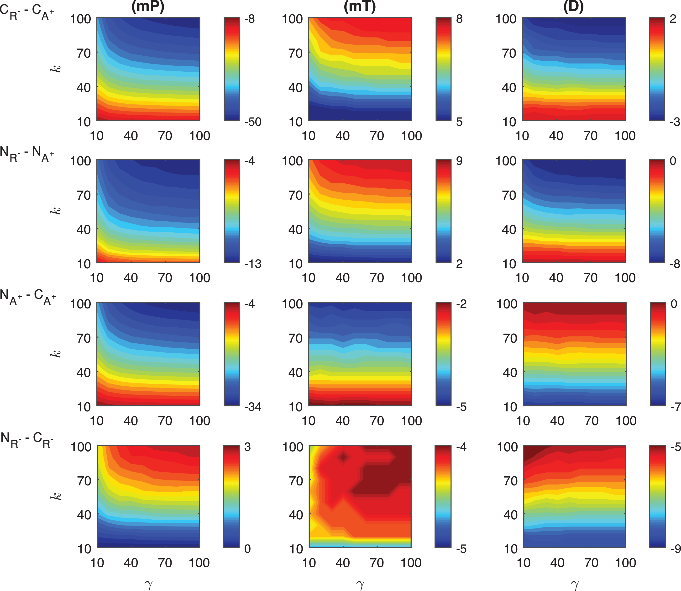
Fig.A.9
Heat maps for the comparison of three metrics (mid-protein level mP, time to reach mid-protein level mT and duration D) describing the dynamics of competitive (CA+, CR−) and noncompetitive (NA+, NR−) activation mechanisms. In these simulations, the signal amplitude γ and persistency k range from a 10-fold to a 100-fold change when ro = 0.01. All the other parameters were held constant at their values listed in Section 3.
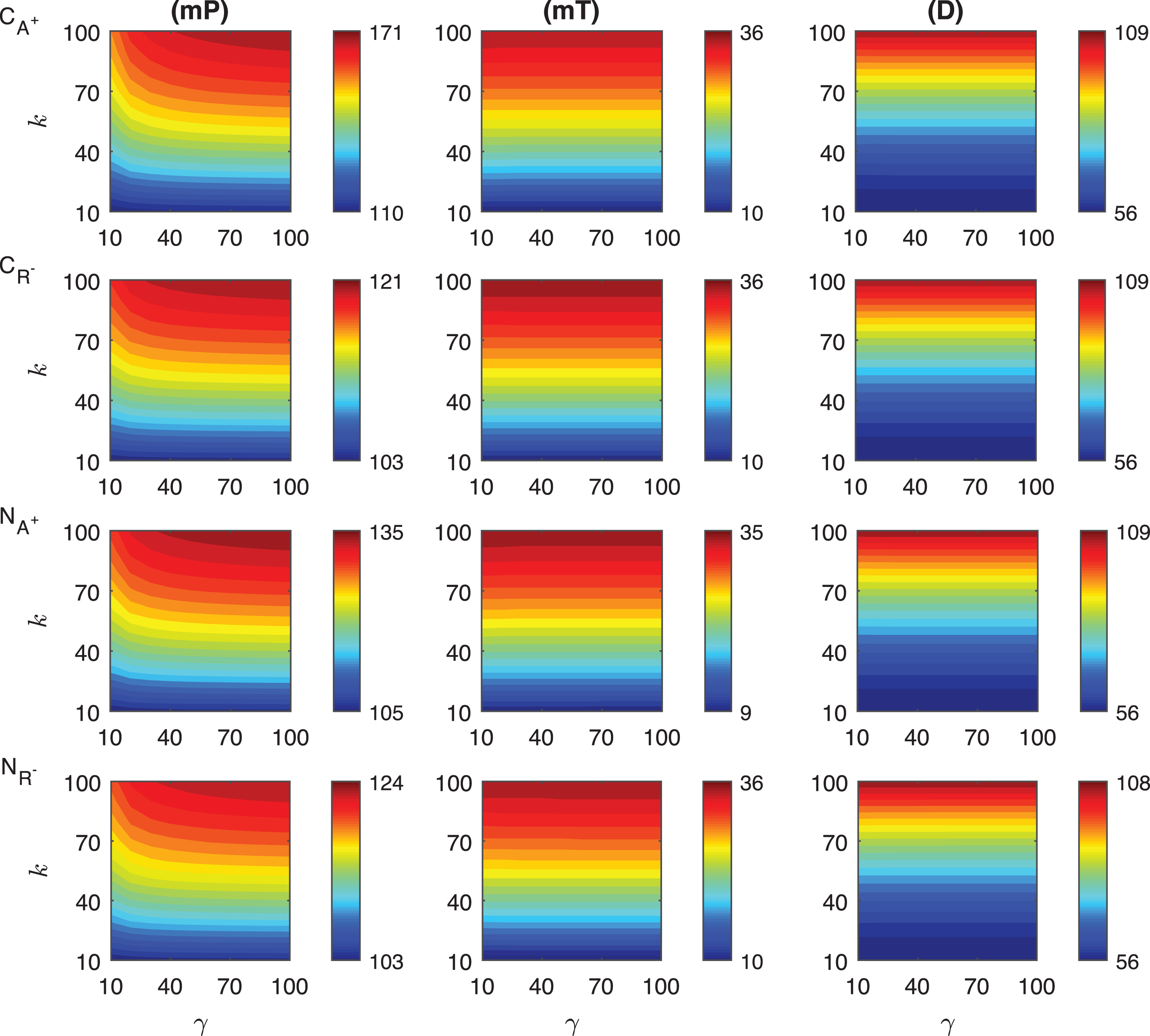
Fig.A.10
Heat maps for the comparison of the differences of three metrics (mid-protein level mP, time to reach mid-protein level mT and duration D) showing the dynamics of competitive (CA+, CR−) and noncompetitive (NA+, NR−) activation mechanisms. For all these simulations, the signal amplitude γ and persistency k are changed from 10-100 fold when ro = 0.01 while all the other parameters were kept constant at their estimated values listed in Section 3.
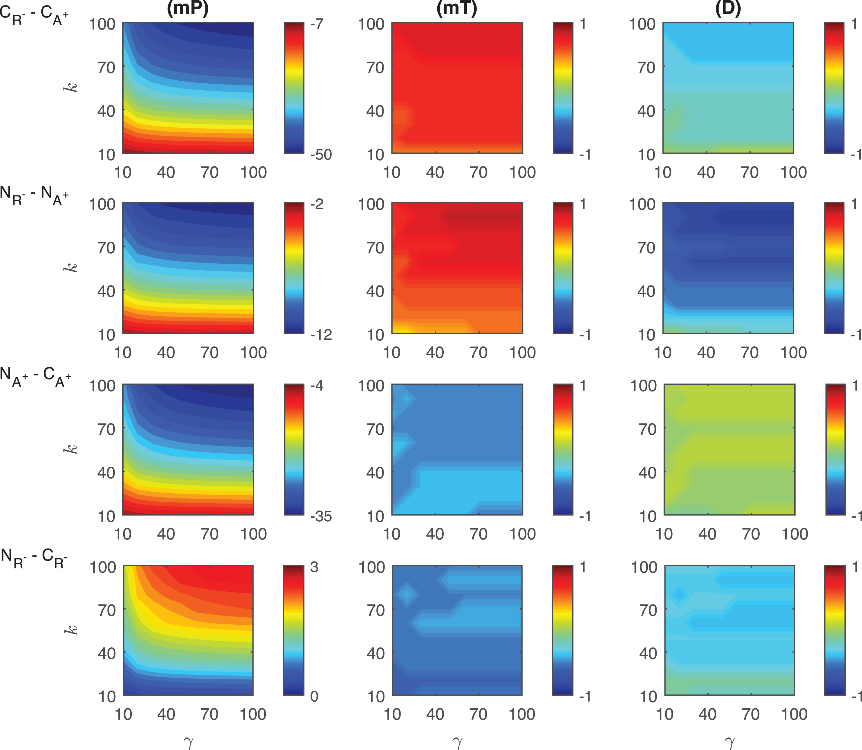
Fig.A.11
Heat maps for the comparison of three metrics (mid-protein level mP, time to reach mid-protein level mT and duration D) describing the dynamics of competitive (CA+, CR−) and noncompetitive (NA+, NR−) activation mechanisms. In these simulations, the signal amplitude γ and persistency k range from a 10-fold to a 100-fold change when ro = 0.1. All the other parameters were held constant at their values listed in Section 3.
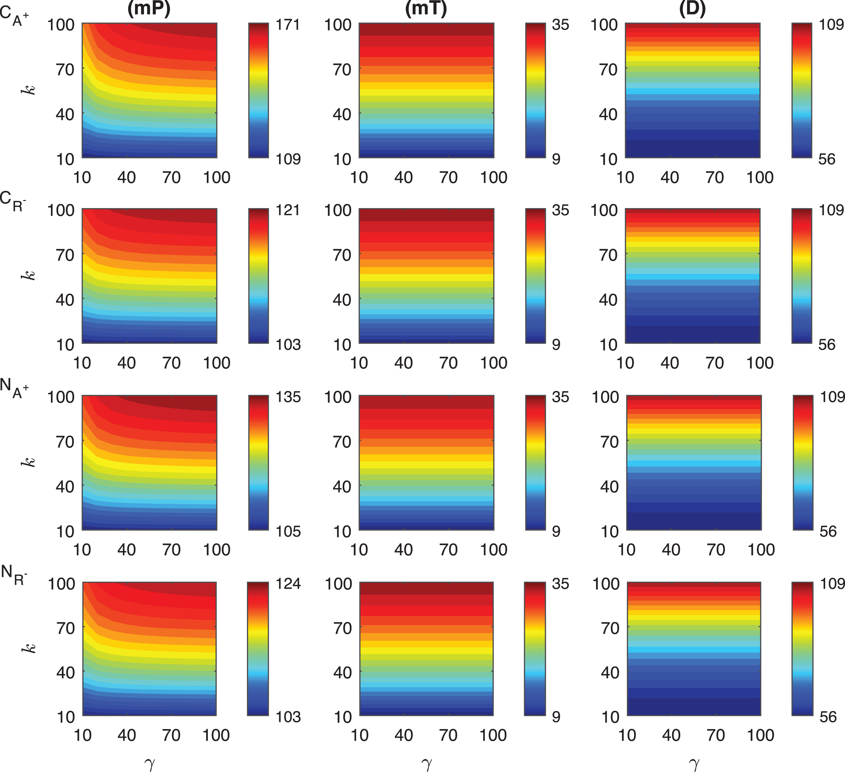
Fig.A.12
Heat maps for the comparison of the differences of three metrics (mid-protein level mP, time to reach mid-protein level mT and duration D) showing the dynamics of competitive (CA+, CR−) and noncompetitive (NA+, NR−) activation mechanisms. For all these simulations, the signal amplitude γ and persistency k are changed from 10-100 fold when ro = 0.1 while all the other parameters were kept constant at their estimated values listed in Section 3.
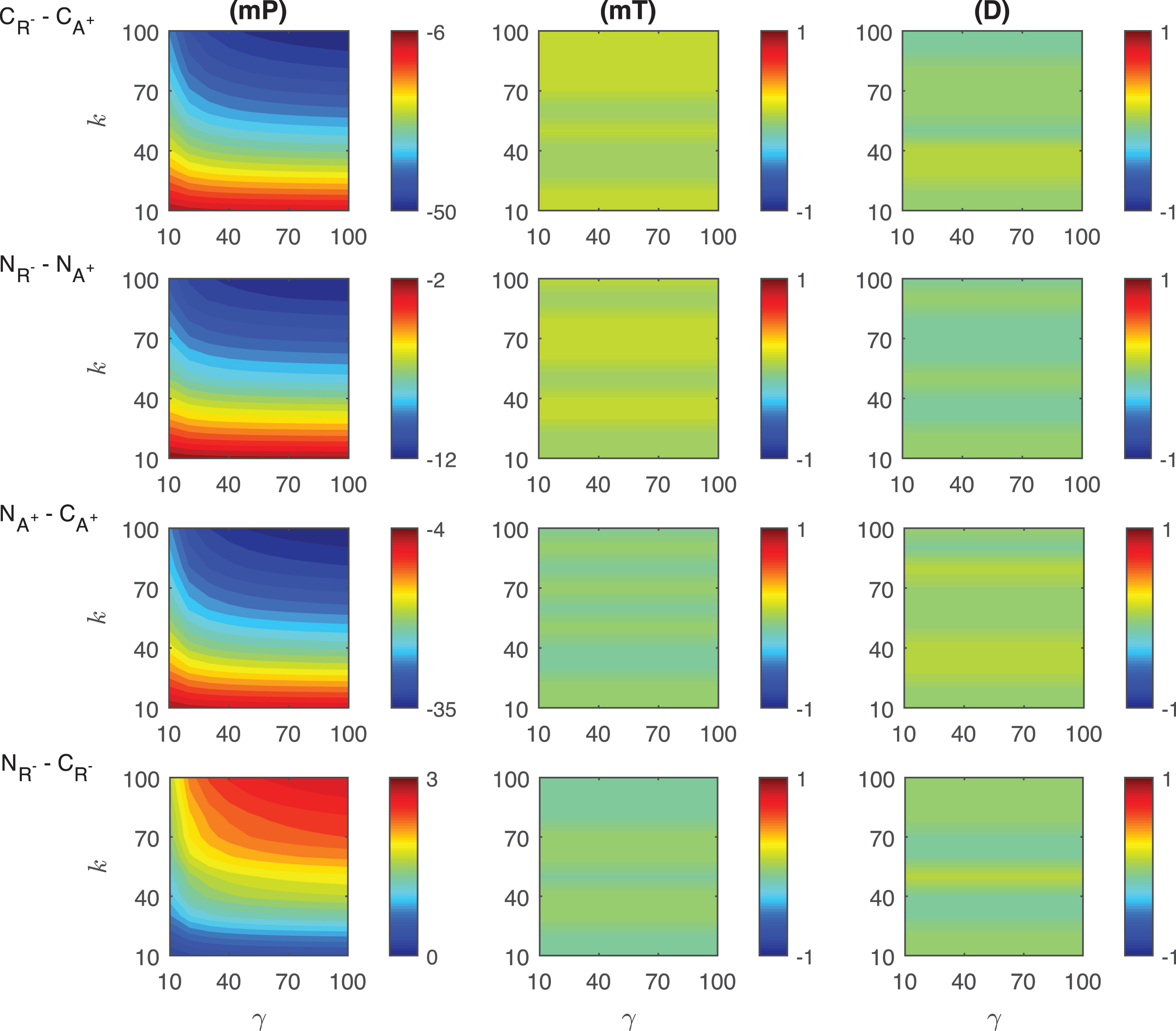
Table A.1
Competitive Summary of the biochemical reactions and reaction rates for the competition model
| Biochemical Reactions | Descriptions | Reaction Rates |
|
| Gene Repression | v1 = roGR, v2 = rfGR |
|
| Gene Activation | v3 = aoGA, v4 = afGA |
|
| mRNA Transcription by GA |
|
|
| mRNA Transcription by G | v6 = ηm0Gτm |
|
| Protein Translation | v7 = αpMτp |
|
| mRNA Degradation | v8 = βmM |
|
| Protein Degradation | v9 = βpP |
|
| ||
Table A.2
NoncompetitiveSummary of the biochemical reactions and reaction rates for the noncompetive model
| Biochemical Reactions | Descriptions | Reaction Rates |
|
| Gene Repression | v1 = roGR, v2 = rfGR |
|
| Gene Activation | v3 = aoGA, v4 = afGA |
|
| Gene Activation/Repression | v8 = aroGAR, v9 = arfGAR |
|
| Gene Activation/Repression | v10 = raoGRA, v11 = rafGAR |
|
| mRNA Transcription |
|
|
| mRNA Transcription | v6 = αm0Gτm |
|
| mRNA Transcription |
|
|
| Protein Translation | v12 = αpMτp |
|
| mRNA Degradation | v13 = βmM |
|
| Protein Degradation | v14 = βpP |
|
| ||
|
| ||
References
[1] | Arnosti D.N. , Analysis and function of transcriptional regulatory elements: Insights from drosophila, Annual Review of Entomology 48: (1) ((2003) ), 579–602. |
[2] | Arnosti D.N. , and Kulkarni M.M. , Transcriptional enhancers: Intelligent enhanceosomes or flexible billboards?, Journal of Cellular Biochemistry 94: (5) ((2005) ), 890–898. |
[3] | Ay A. , and Arnosti D.N. , Mathematical modeling of gene expression: A guide for the perplexed biologist, Critical Reviews in Biochemistry and Molecular Biology 46: (2) ((2011) ), 137–151. |
[4] | Ay A. , Wilner N. , and Yildirim N. , Mathematical modeling deciphers the benefits of alternatively-designed conserved activatory and inhibitory gene circuits, Molecular BioSystems 11: ((2015) ), 2017–2030. |
[5] | Bernstein J.A. , Lin P.-H. , Cohen S.N. , and Lin-Chao S. , Global analysis of escherichia coli rna degradosome function using dna microarrays, Proceedings of the National Academy of Sciences of the United States of America 101: (9) ((2004) ), 2758–2763. |
[6] | Bremer H. , and Dennis P.P. , et al. Modulation of chemical composition and other parameters of the cell by growth rate, Escherichia Coli and Salmonella: Cellular and Molecular Biology 2: ((1996) ), 1553–1569. |
[7] | Laat W.D. , and Duboule D. , Topology of mammalian developmental enhancers and their regulatory landscapes, Nature 502: (7472) ((2013) ), 499–506. |
[8] | Fakhouri W.D. , Ay A. , Sayal R. , Dresch J. , Dayringer E. , and Arnosti D.N. , Deciphering a transcriptional regulatory code: Modeling short-range repression in the drosophila embryo, Molecular Systems Biology 6: (1) ((2010) ), 341. |
[9] | Ferraris L. , Stewart A.P. , Kang J. , DeSimone A.M. , Gemberling M. , Tantin D. , and Fairbrother W.G. , Combinatorial binding of transcription factors in the pluripotency control regions of the genome, Genome Research 21: (7) ((2011) ), 1055–1064. |
[10] | Finkel T. , and Gutkind J.S. , Signal transduction and human disease. Wiley Online Library, (2003) . |
[11] | Gillespie D.T. , Exact stochastic simulation of coupled chemical reactions, J Phys Chem 81: ((1977) ), 2340–2361. |
[12] | Gupta C. , López J.M. , Ott W. , Josic K. , and Bennett M.R. , Transcriptional delay stabilizes bistable gene networks, Physical Review Letters 111: (5) ((2013) ), 058104. |
[13] | Ishihama Y. , Schmidt T. , Rappsilber J. , Mann M. , Hartl F.U. , Kerner M. , and Frishman D. , Protein abundance profiling of the escherichia coli cytosol, BMC Genomics 9: (1) ((2008) ), 102. |
[14] | Jaeger J. , Surkova S. , Blagov M. , Janssens H. , Kosman D. , Kozlov K.N. , Myasnikova E. , Vanario-Alonso C.E. , Samsonova M. , and Sharp D.H. , et al. Dynamic control of positional information in the early drosophila embryo, Nature 430: (6997) ((2004) ), 368–371. |
[15] | Janssens H. , Hou S. , Jaeger J. , Kim A.-R. , Myasnikova E. , Sharp D. , and Reinitz J. , Quantitative and predictive model of transcriptional control of the drosophila melanogaster even skipped gene, Nature Genetics 38: (10) ((2006) ), 1159–1165. |
[16] | Jones B. , Stekel D. , Rowe J. , and Fernando C. , Is there a liquid state machine in the bacterium?, In Artificial Life, 2007 ALIFE’07 IEEE Symposium on, IEEE (2007) , pp. 187–191. |
[17] | Kærn M. , Elston T.C. , Blake W.J. , and Collins J.J. ,, Stochasticity in gene expression: From theories to phenotypes, Nature Reviews Genetics 6: (6) ((2005) ), 451–464. |
[18] | Kennell D. , and Reizman H. , Transcription and translation initiation frequencies of thelac operon, J Mol Biol 114: ((1977) ), 1–21. |
[19] | Kepler T.B. , and Elston T.C. , Stochasticity in transcriptional regulation: Origins, consequences, and mathematical representations, Biophys J 81: ((2001) ), 3116–3136. |
[20] | Levo M. , and Segal E. , In pursuit of design principles of regulatory sequences, Nature Reviews Genetics 15: (7) ((2014) ), 453–468. |
[21] | Mackey M.C. , Tyran-Kaminska M. , and Yvinec R. , Dynamic behavior of stochastic gene expression models in the presence of bursting, SIAM Journal on Applied Mathematics 73: (5) ((2013) ), 1830–1852. |
[22] | Makeev V.J. , Lifanov A.P. , Nazina A.G. , and Papatsenko D.A. , Distance preferences in the arrangement of binding motifs and hierarchical levels in organization of transcription regulatory information, Nucleic Acids Research 31: (20) ((2003) ), 6016–6026. |
[23] | Monar H. , Goodman D. , and Stnet G.S. , RNA chain growth rates in, J Mol Biol 39: ((1969) ), 1–29. |
[24] | Munteanu A. , Constante M. , Isalan M. , and Solé R.V. , Avoiding transcription factor competition at promoter level increases the chances of obtaining oscillation, BMC Systems Biology 4: (1) ((2010) ), 1. |
[25] | Yildirim N. , and Mackey M.C. , Feedback regulation in the lactose operon: A mathematical modeling study and comparison with experimental data, Biophysical Journal 84: ((2003) ), 84. |
[26] | O’Neill L.A.J. , Targeting signal transduction as a strategy to treat inflammatory diseases, Nature Reviews Drug Discovery 5: (7) ((2006) ), 549–563. |
[27] | Romero I.G. , Ruvinsky I. , and Gilad Y. , Comparative studies of gene expression and the evolution of gene regulation, Nature Reviews Genetics 13: (7) ((2012) ), 505–516. |
[28] | Rothschild D. , Dekel E. , Hausser J. , Bren A. , Aidelberg G. , Szekely P. , and Alon U. , Linear superposition and prediction of bacterial promoter activity dynamics in complex conditions, PLoS Comput Biol 10: (5) ((2014) ), e1003602. |
[29] | Rué P. , and Jordi Garcia-Ojalvo. Modeling gene expression in time and space, Annual Review of Biophysics 42: ((2013) ), 605–627. |
[30] | Samee M.A.H. , Lim B. , Samper N. , Lu H. , Rushlow C.A. , Jiménez G. , Shvartsman S.Y. , and Sinha S. , A systematic ensemble approach to thermodynamic modeling of gene expression from sequence data, Cell Systems 1: (6) ((2015) ), 396–407 . |
[31] | Sarkar R.R. , Maithreye R. , and Sinha S. , Design of regulation and dynamics in simple biochemical pathways, Journal of Mathematical Biology 63: (2) ((2011) ), 283–307. |
[32] | Sayal R. , Dresch J.M. , Pushel I. , Taylor B.R. , and Arnosti D.N. , Quantitative perturbation-based analysis of gene expression predicts enhancer activity in early drosophila embryo, eLife 5: ((2016) ), e08445. |
[33] | Segal E. , Raveh-Sadka T. , Schroeder M. , Unnerstall U. , and Gaul U. , Predicting expression patterns from regulatory sequence in drosophila segmentation, Nature 451: (7178) ((2008) ), 535–540. |
[34] | Shen-Orr S.S. , Milo R. , Mangan S. , and Alon U. , Network motifs in the transcriptional regulation network of escherichia coli, Nature Genetics 31: (1) ((2002) ), 64–68. |
[35] | So L.-H. , Ghosh A. , Zong C. , Sepúlveda L.A. , Segev R. , and Golding I. , General properties of transcriptional time series in escherichia coli, Nature Genetics 43: (6) ((2011) ), 554–560. |
[36] | Taniguchi Y. , Choi P.J. , Li G.-W. , Chen H. , Babu M. , Hearn J. , Emili A. , and Xie X.S. , Quantifying} proteome and transcriptome with single-molecule sensitivity in single cells, Science 329: (5991) ((2010) ), 533–538. |
[37] | Roey K.V. , and Davey N.E. , Motif co-regulation and co-operativity are common mechanisms in transcriptional, post-transcriptional and post-translational regulation, Cell Communication and Signaling 13: (1) ((2015) ), 1. |
[38] | Wang C. , Yi M. , Yang K. , and Yang L. , Time delay induced transition of gene switch and stochastic resonance in a genetic transcriptional regulatory model,S, BMC Systems Biology 6: (Suppl 1) ((2012) ), 9. |
[39] | Wang X. , Hao N. , Dohlman H.G. , and Elston T.C. , Bistability, stochasticity, and oscillations in the mitogen-activated protein kinase cascade, Biophysical Journal 90: (6) ((2006) ), 1961–1978. |
[40] | Wittkopp P.J. , and Kalay G. , Cis-regulatory elements: Molecular mechanisms and evolutionary processes underlying divergence, Nature Reviews Genetics 13: (1) ((2012) ), 59–69. |
[41] | Wong P. , Gladney S. , and Keasling J.D. , Mathematical model of the lac operon: Inducer exclusion, catabolite repression, and diauxic growth on glucose and lactose, Biotechnol Prog 13: ((1997) ), 132–143. |
[42] | Yvinec R. , Zhuge C. , Lei J. , and Mackey M.C. , Adiabatic reduction of a model of stochastic gene expression with jump markov process, Journal of Mathematical Biology 68: (5) ((2014) ), 1051–1070. |
[43] | Zeitlinger J. , Zinzen R.P. , Stark A. , Kellis M. , Zhang H. , Young R.A. , and Levine M. , Whole-genome chip–chip analysis of dorsal, twist, and snail suggests integration of diverse patterning processes in the drosophila embryo, Genes & Development 21: (4) ((2007) ), 385–390. |


