
Modelling speciation: Problems and implications
Abstract
Darwin’s and Wallace’s 1859 explanation that novel speciation resulted from natural variants that had been subjected to selection was refined over the next 150 years as genetic inheritance and the importance of mutation-induced change were discovered, the quantitative theory of evolutionary population genetics was produced, the speed of genetic change in small populations became apparent and the ramifications of the DNA revolution became clear. This paper first discusses the modern view of speciation in its historical context. It then uses systems-biology approaches to consider the many complex processes that underpin the production of a new species; these extend in scale from genes to populations with the processes of variation, selection and speciation being affected by factors that range from mutation to climate change. Here, events at a particular scale level (e.g. protein network activity) are activated by the output of the level immediately below (i.e. gene expression) and generate a new output that activates the layer above (e.g. embryological development), with this change often being modulated by feedback from higher and lower levels. The analysis shows that activity at each level in the evolution of a new species is marked by stochastic activity, with mutation of course being the key step for variation. The paper examines events at each of these scale levels and particularly considers how the pathway by which mutation leads to phenotypic variants and the wide range of factors that drive selection can be investigated computationally. It concludes that, such is the complexity of speciation, most steps in the process are currently difficult to model and that predictions about future speciation will, apart from a few special cases, be hard to make. The corollary is that opportunities for novel variants to form are maximised.
1Introduction
Research into evolution naturally falls into two categories. The first is to discover the history of life that dates back to the Last Universal Common Ancestor (LUCA), a primitive prokaryote. This evolved from the First Universal Common Ancestor, a very primitive bacterium that formed about 3.8 billion years ago (Ba) about which our knowledge can only be informed speculation. The second is the study of the mechanisms by which new species evolve from parent species. The history of life is now generally understood on the basis of phylogenetic analysis and, for larger organisms, fossil analysis (see [1] for general review). Unpicking the details of the mechanisms of evolutionary change is however much harder as they not only include strong stochastic components but are frequently hard to define with any degree of precision. This is partly because so much is going on and partly because we cannot assume that conditions stay the same over the long periods that are needed for a new species to form from a parent species.
It is not even straightforward to define a species. Although we normally think of species as being distinct if they look different in some way, this definition is not always applicable: the many breeds of dogs, from dachshunds to Great Danes, are all the same species. There are many other definitions [2], but the best reflects reproduction. Here, species are different if any hybrids that might form are incapable of leaving fertile offspring. The importance of this definition is that it drives irreversible diversification. This breakdown does, however, usually depend on the hybrid’s chromosomes being unable to pair during meiosis and, in the case of animals that mate directly, is rarely achieved until long after the two populations have lost interest in crossbreeding (see below).
Unfortunately, the reproductive test is usually impractical to apply to most pairs of living species and of course impossible for those that are extinct. The usual definitions are therefore that species are different either if they have sufficiently different features (this normally means that they have qualitative rather than quantitative differences) or if they are incapable of living in the same habitat. Such definitions do not usually work for organisms such as prokaryotes, many of which look the same; here one may be forced to consider definitions based on genomic differences.
The main purpose of this paper is to consider the extent to which novel speciation can be quantitatively modelled. While it starts with a brief summary of the successes that have been achieved in modelling the history of species diversification, the bulk of the paper focuses on the mechanisms that underly change and is in in two parts. The first sets out in a historical context our current understanding of how evolutionary change is initiated and how it culminates in the formation of a new species as recognised on the basis of anatomical differences. The second looks at the various aspects of these processes and the difficulties in modelling them quantitatively.
2The history of life
Our understanding of the history of life dates back to Jean-Baptist Lamarck who, in 1809, analysed the very different anatomies of annelid worms and parasitic flatworms. His conclusion was that their separate evolution could not have occurred by climbing the ladder of complexity from protist to humans, as had been suggested by Bonnet in the late 18th century, but had to have been the result of branching descent [3]. Early studies confirmed this and unpicked much of vertebrate history through analysis of the fossil record. By the 1960 s, it became possible to formalise this within the framework of cladistic hierarchies: these are directed graphs, whose nodes are species and whose edges are defined by the relationship descends with modification from [1].
Theoretical modelling of the history of life took a major leap forward in the early 1970 s with the availability of first protein and then DNA sequences. These stimulated computer scientists to produce algorithms that analysed homologous sequences on the basis of mutational differences. The resulting analysis of the vast amounts of sequence data now available has, over the last few decades, produced detailed phylogenies for all the major and most of the minor clades: these group contemporary organisms and identify lines of descent leading back to common ancestors and eventually to the Last Eukaryotic Common Ancestor (LECA –the accepted name for the first organism with a nucleus). These molecular phylogenies are not only more precise than anatomical phylogenies (cladograms) based on the fossil record but can be derived for any group of species for which there is adequate DNA sequence data.
Comparative sequence algorithms have also been used on prokaryotic sequence data to show how the LECA formed as the result of the endosymbiosis of several ancient members of modern families of Eubacteria and Archaebacteria [1]. This has now given us a reasonable picture of the Last Universal Common Ancestor (LUCA), a very simple bacterium that was the unique parent of every living cellular organism. As a result of all this work, we now know the general history of every living organism that has been studied (for a summary, see [1]; for details, see the Wikipedia entry for any organism).
The details of this history are of course limited because molecular phylogenetics can only group contemporary organisms and identify branch points that represent early common ancestors. The identification of extinct taxa, which can be located within cladograms, are restricted to animals and plants for which there is a substantial fossil record. We do however have an independent test of the accuracy of this phylogeny: this comes from the many observations showing that homologous proteins have homologous functions even in distantly related organisms, usually during development (the area of research called evo-devo). For instance, every animal with an eye expresses a homologue of the Pax6 protein at an early stage in its development [4].
It should also be emphasised that the cladograms and molecular phylograms that summarise the history of life reflect graphs with very low time resolution. This is partly because the fossil record is inevitably limited [5] and partly because they inevitably lack short-term detail. If one examines any phylogram, there is a sense of inevitability when one follows a line of evolutionary descent from one node to another. The reality is very different: if one were to look closely at what happens at a specific node, one would see a broad range of descent lines as the variants of some species tried, as it were, their luck in one or more environments with different selection pressures (see below).
What normally happens is that all but one line in this bush dies out and a single species is successful, although there is no reason in principle why a single population cannot give rise to several successful lines, provided that each finds itself in a novel environment. The difficulty is that the time needed for this success could well extend to thousands of generations (e.g. the Neanderthals survived for > 300K years or 15K generations). Even then, most trait variants that seem beneficial in the short term die out in the medium term, so that what appears in a low-time-resolution phylogram is a solitary success. The paradigm here is us: the Hominini clade originated some 7 Mya and slowly branched to give a bush of taxa of which the sole surviving member is Homo sapiens [6], albeit that its genome contains fragments from other bush taxa as a result of interbreeding.
Although there is always more detail to be explored, our understanding of the general history of eukaryotic life is now robust. Our knowledge of prokaryotic evolution is thinner: we still lack full understanding about the FUCA evolved and the nature of the last common ancestor of the Eubacterium and the Archaebacterium clades, while it is still hard to make plausible predictions about the future for organisms more complex than infectious viruses [7]. Before considering the mechanistic side of evolution, however, all biologists should thank the mathematicians who invented the algorithms and statistical methodologies for making molecular phylogenies; they have revolutionised our understanding of the history of life.
3The mechanisms of evolutionary change
Our knowledge of the mechanisms by which new species evolve from parent species is inevitably thinner than that for elucidating the broad line of evolutionary history as the details of how each new species forms are specific to that species. Lamarck suggested that variants arose through organisms having the ability to become more complex and to improve their abilities through effort, with the acquired characteristics being heritable [3]. This view was widely held until the end of the nineteenth century when Weismann showed that, as the germ cells were separated from the body early in development, there was no known way in which novel phenotypic characteristics in the adult could feed back to germ cells.
In the 1830 s, Darwin started to explore evidence for the idea that novel speciation derived from natural variants (he accepted Lamarck’s views on the origins of variation) that were subject to selection either through pressures from the environment in which they lived (natural selection) or through an enhanced ability to procreate (sexual selection). Publication of this work was forced by Darwin’s receipt of a manuscript in 1858 from Wallace, who had had similar ideas when he had been ill in Indonesia. Later that year, side-by-side papers were published [8] and, the following year, Darwin published On the origin of species [9]. This book summarised the evidence for his views on how new species formed, but actually said little on how a species can be defined or a new one recognised.
3.1How do new species originate?
Darwin’s answer to this question was that new species form from a succession of natural variants that breed better (or are fitter) than their parents in a particular environment. Eventually, the changes are sufficient that a new species forms that is unable to breed with its parent species and may well supersede it through natural selection. Evidence to support this answer comes from what are known as ring species. These form when a migrating population meets an inhospitable domain and therefore divides, with some going left and others right, each group undergoing variation over time. In a few cases, the groups eventually meet up forming a ring of distinct variants. An important observation on these is that, while any left- or right-migrating population can successfully mate with its immediate neighbours and so are just subspecies, the terminal left and right populations may not interbreed and thus have to be seen as distinct species. There are several examples of ring species that include the greenish warbler family of birds that surround the Himalayas (Fig. 1), the herring gulls around the Arctic and the Euphorbia plants around the Caribbean (for references, see [10]) and the Wikipedia entry on Ring Species).
Fig. 1
Ring species. The greenish warblers (Phylloscopus trochiloides) were originally present in the region south of the Himalayas. They slowly spread east and west forming a series of distinct species, eventually meeting up in Siberia to form a ring. All neighbouring species will interbreed except for those on either side of the meeting point. This seems to be because theirs songs are too different for the two species to recognise one another [6]. (Main image: Courtesy of G. Ambrus. Inserts: phylloscopus trochiloides: Courtesy of P. Jaganathan. P. t. plumbeitarsus: courtesy of Ayuwat Jearwattanakanok. P. t. viridanus: Courtesy of Dibenu Ash. (Other images published under a CC Attribution -Share Alike 3.0 unported License.)
![Ring species. The greenish warblers (Phylloscopus trochiloides) were originally present in the region south of the Himalayas. They slowly spread east and west forming a series of distinct species, eventually meeting up in Siberia to form a ring. All neighbouring species will interbreed except for those on either side of the meeting point. This seems to be because theirs songs are too different for the two species to recognise one another [6]. (Main image: Courtesy of G. Ambrus. Inserts: phylloscopus trochiloides: Courtesy of P. Jaganathan. P. t. plumbeitarsus: courtesy of Ayuwat Jearwattanakanok. P. t. viridanus: Courtesy of Dibenu Ash. (Other images published under a CC Attribution -Share Alike 3.0 unported License.)](https://content.iospress.com:443/media/isb/2023/15-1-2/isb-15-1-2-isb220253/isb-15-isb220253-g001.jpg)
Although Darwin’s view of speciation is basically correct, it is very thin and says nothing about either how variants arise or how they are propagated within a population under selection. At around the end of the 19th century, the rediscovery of Mendel’s 1866 paper [11], with its basic laws of genetics and the idea that genes underpinned phenotypes, stimulated mathematicians to work through the ways in which these laws could be applied to populations that were evolving. Around 1907, Hardy and Weinberg independently showed that, in the absence of selection or migration, gene frequencies would not change over the generations. A decade later, Fisher had produced a substantial mathematical model of evolutionary population genetics that showed how change could happen in diploid organisms that reproduced sexually. This theory covered selection, the spread of novel alleles and how the effects of several alleles in a gene could explain continuous variation in a phenotypic trait such as height [12]. It was a remarkable and brilliant piece of work.
Over the next few decades, this model was expanded to explain much of how genes spread through populations under selection and other factors such as genetic drift (effects of random gene distributions in small populations –see below). The integration of population genetics and Darwinian selection gave what came to be called the modern evolutionary synthesis [see [13] for a summary of its various components). Its most robust achievement has been to show quantitatively how mutations move through populations and how the details of this movement depend on population size, selection (natural, sexual and kin), immigration and other such factors.
All this remarkable work was of course done in the absence of any knowledge of what a gene was or how it worked, although it was clear that mutations were the basic cause of variation. It also said very little about how speciation was achieved. Enough was however known to pose the two key problems in a far richer context than had previously been possible. The first was how mutations led to changes in the phenotype; the second was how successful variants led to new species. These problems are still not fully answered for the great majority of species, even in the light of contemporary knowledge of molecular and developmental biology. Nevertheless, the quantitative theory still provides a framework for thinking about evolutionary change and is an important component of coalescent analysis, which uses sets of DNA sequences and a model of population breeding behaviour to produce numerical details of ancient populations [14].
There are however weaknesses in the mathematical model of evolutionary genetics. First, its emphasis is inevitably on the short-term movement of genes under a constant set of criteria from one equilibrium position to another –it cannot model longer-term events into the future unless conditions remain unaltered over very long periods. Second, its view of the relationship between genotype and phenotype was, and remains, naïve: it assumes that this is direct in that one or at most a few genes that may interact (i.e., show epistasis) are responsible for a particular phenotype and that alleles of those genes underpin alternative phenotypes. This is sometimes true, as Mendel showed for peas, but such Mendelian genes are relatively rare, other than in the case of mutants that lead to genetic disease, and these are unlikely candidates for driving evolutionary change. Modern molecular genetics has shown that most aspects of an organism’s phenotype are underpinned by sets of genes whose proteins cooperate within networks (see below). If the speed of horses was the result of Mendelian genes, racehorse-breeding would be far more reliable than it is! Third, the model requires numerical parameters for its equations, and these can be hard to measure.
3.2The modern view of speciation
Originally, evolutionary population geneticists assumed that, if enough novel and favourable mutations accumulated within a population, a new species would form from the original one. It soon became clear, however, that selection would have to be very strong if a novel mutation was not to be lost in a growing population. During the 1950 s and ‘60 s, a group of geneticists, key members of which were Ernst Mayr and Motoo Kimura, showed that this effect could be overcome in small populations. One reason for this is because genetic drift, which reflects random assortment of gene distributions during breeding, becomes disproportionately important as population numbers decrease ([15] and see below).
When a small population becomes isolated from its parent population, it has a pangenome (the complete set of genes and allelic variants in a population) that is a random, asymmetric subset of the parent profile. Such a small, isolated population that finds itself in a novel environment will frequently die out because it is unfit for the new selection pressures that it encounters. If, however, a subgroup within the small population has an allele distribution that allows it to survive, it will become a new founder population (Fig. 2). In this case, differences between this and the original population will increase more rapidly than might be expected for a series of reasons that are detailed in Box 1. It is also worth noting that, as normal mutation rates are very slow, most new variants derive from novel mixes of existing mutations rather than the formation of new ones (see below).
Fig. 2
The process by which a new species eventually when a small founder population breaks away from a parent population (From [1], with permission).
![The process by which a new species eventually when a small founder population breaks away from a parent population (From [1], with permission).](https://content.iospress.com:443/media/isb/2023/15-1-2/isb-15-1-2-isb220253/isb-15-isb220253-g002.jpg)
Box1: The unique genetic properties of small groups
| 1. As numbers are small, the random effects of genetic drift in breeding are more important than the deterministic predictions of Mendelian laws. |
| 2. Breeding within this asymmetric and diminished gene population leads to a loss of heterozygosity and an increased number of recessive phenotypes (the Wahlund effect). |
| 3. Because such groups probably included families, the likelihood of incestuous mating will be increased. This would result in a further loss of heterozygosity and an increased likelihood of recessive homozygotes forming. |
| 4. In small as compared to large populations, genetic change is likelier to happen and be taken up much faster. In these cases, gene alleles that lead to a favoured phenotype (and enhanced fitness) would rapidly come to predominate, while deleterious ones would soon be lost. |
| 5. Small populations are genetically robust against the acquisition of deleterious mutations [11]. |
In an environment with selection pressures different from those of the parent environment, new phenotypic characteristics will slowly appear over time in the descendants of the founder population, mainly as a result of the original asymmetric allele distribution, genetic drift and new mutations; the phenotype distribution of the population will consequently change. As these effects are occurring, larger chromosomal changes will also slowly take place so that the new and the parent organisms would, were they to meet, become increasingly less likely over time to produce fertile offspring. Eventually, all such hybrids would fail, and the two populations will have become different species. The example of mules shows how slow this process is: the very occasional mule is still fertile even though the horse and donkey lines separated some 2 million years ago (Mya), a figure that represents about a million generations [16–18].
While this view of speciation has had major experimental and theoretical successes, it is worth pointing out that some in the field have felt for some time that its broad-brush approach lacks several important features that facilitate novel speciation. They have therefore put forward the Extended evolutionary synthesis that contains mechanisms beyond routine mutation and selection that are not explicitly included in the standard synthesis [19]. These include transgenerational epigenetic inheritance and developmental plasticity to extend the repertoire of novel trait formation and multilevel selection, niche construction and punctuated equilibrium all of which have the general ability to speed up the speciation process. The importance of these factors is obvious and many feel that they are implicitly included in the Modern Synthesis; they are not however considered here partly because their individual contributions to novel speciation are unclear and partly because they cannot yet be quantified.
4The modelling problems
While there is no reason to doubt this general picture of speciation of how a subpopulation of a parent population becomes increasingly distinct and eventually a new species, its broadness hides a range of complexities in both the variation and selection components of change. For variation, the most obvious reflect new beneficial mutations, although these are very slow to appear. Far more important in the short term is the stochastic assortment of existing mutations that occurs first in meiosis and then in random breeding within a population. Experimental studies of phenotypic changes in populations have clearly shown that novel mixes of existing gene alleles are predominantly responsible for producing at least the initial stages of new phenotypes [20, 21].
The direct effect of any mutations on phenotypes, except for those in Mendelian genes, are however hard to predict or even understand. In the case of proteins, mutations in their sequences generally alter the binding and activation constants of proteins with other proteins and with substrates. As a result, their effects are disseminated across any networks in which they are involved (see below). In the case of mutations that affect protein-regulatory regions, the effect can be to change gene expression and hence protein concentrations, again in ways that cannot be anticipated only analysed. Equally unpredictable and important in the much longer term are the accumulation of speciation genes and chromosomal rearrangements in the two populations that will eventually render infertile any hybrids that might form.
There are also problems associated with the effects of selection on populations, a process that reflects interactions with other organisms, with their mix of traits, together with the effects on them of their environment. Selection in the wild is particularly complicated as it includes interactions with other organisms, predators, food supplies and the effects of climate. Such complexity makes modelling difficult, particularly because any aspect of the process can change during the long periods over which speciation takes place. A further difficulty is that, ab initio, we generally have little idea of the trajectory of change or its endpoint except under experimental conditions where selection can be controlled and the specific case of mimicry (Anthony Flemming, personal communication). Hindsight is far easier than foresight!
Table 1 summarises the many events that together lead to novel speciation and it is worth noting that each includes aspects that are not predictable. Most reflect random events at a particular level of scale, while some, such as the complex effects of selection in the wild, reflect downwards control from a higher to a lower level (Fig. 3). A few, however, reflect emergent properties that are generated when events at one level, which is particularly complex, produce results at a higher level that could not have been predicted. Important examples here are the ways that mutations within protein networks generate unexpected phenotypes during development, and the unexpected allele combinations that arise in small populations with limited genomes [22, 23]. These trans-level interactions (Fig. 3) add further degrees of complexity at each level.
Table 1
The steps from a founder population to a new species
| EP: Emergent properties. R: Random, stochastic events. UE: unpredictable events. |
| Immediate effects (up to a few generations) |
| Segregation of small, founder populations from parent ones. R |
| (These populations have limited pangenomes. R) |
| Random crossover during meiosis. R |
| Random allele distribution as a result of normal and incestuous breeding. R |
| Short term (up to a hundred generations) |
| Genotype |
| Because numbers are small, breeding results in a loss of heterozygosity and an |
| increased number of recessive homozygotes. UE |
| Phenotype |
| Possibility of unexpected phenotypes through novel allele combinations and random drift. EP |
| Acquisition of behavioural traits that discourage interbreeding with parent group. R |
| Medium term (hundreds-thousands of generations) |
| Genotype |
| Novel mutations that are different in parent and founder populations. R |
| Phenotype |
| New phenotype variants. EP |
| Success of variants under selection (natural, sexual, kin). UP |
| Increasing divergence of daughter and parent populations. |
| Decrease in hybrid fertility. |
| Long term (Millions of generations) |
| Genotype |
| Formation of chromosome abnormalities. R |
| Phenotype |
| Hybrids between the descendants of the founder and parent populations are infertile. |
Fig. 3
The scale hierarchy shows the key levels through which the effects of a mutation work their way up from the genome to the individual way. Note that there are feedback interactions, both up and down, between the levels. (From [1], with permission.)
![The scale hierarchy shows the key levels through which the effects of a mutation work their way up from the genome to the individual way. Note that there are feedback interactions, both up and down, between the levels. (From [1], with permission.)](https://content.iospress.com:443/media/isb/2023/15-1-2/isb-15-1-2-isb220253/isb-15-isb220253-g003.jpg)
Together, these complexities highlight a deeper problem in modelling: there are no natural endpoints. The processes of variation and selection never cease and there are no criteria for when novelty becomes stable. The only buffer against change is a large breeding population: evolutionary population genetics has shown that the time required for a new mutation to become part of the wildtype population depends on the number of individuals in that breeding population. Curiously, the species for which this particularly applies is humans [1]: because of migration and interbreeding between groups across the world, the populations size is effectively infinite –we are all part of a single breeding population. In consequence, it is now not only hard to see how a novel mutation that was advantageous could spread, but hard to envisage a mutation that would be reproductively advantageous, given the tendency for women to produce fewer children now than in the past. There is thus an argument for saying that humans are now in a post-evolutionary phase.
The natural framework for considering such complexity is systems biology which, in this context, sets out to understand the complex events associated with each level of the scale hierarchy (Fig. 3) together with the feedback interactions across levels (the role of systems biology in understanding protein networks is discussed below in §5.2). The added effect of cross-level, feedback interactions on the events at a particular level always add complexity to the system, even in stable ecosystems. Evolution considers what happens when the base level, the genome, is perturbed by mutation and how the effects of this mutation are projected up the scale hierarchy. It is however hard to get the full picture of these events for the great majority of eukaryotic organisms.
A great deal of material is available for studying the broad range of evolutionary phenomena. Theoretical approaches include the quantitative theory of evolutionary population genetics; this can be explored using both analytic and simulation approaches, computational phylogenetics, statistical analysis and models based on differential equations and Boolean operators (Section 5.2). The data available for analysis include DNA sequences, details of protein networks, the phenotypic changes generated by mutation, data from population studies, such as the effects of selection, genetic profiles of and breeding behaviour within small groups, the formation and accumulation of major chromosomal changes and the results of experimental studies. It should however be emphasised that, although sequence data for some organisms is complete, its understanding is not, apart from the genomes of viruses and a few bacteria. It is, for example, still impossible to unravel the full genetic basis of any organism’s development and only rarely do we have the full details of how specific mutations lead to variation in the developing anatomical phenotype (for review, see [24]).
Apart from the problems of stochasticity (Table 1), there are other difficulties that any analysis has to confront. An obvious example is that variation requires beneficial changes and these are very much harder to identify than deleterious ones, except with hindsight. In addition, it can be hard to get the numerical constants that modelling requires when the limited data from which these are extracted must also be used to test theoretical predictions. These limitations are particularly important when apparently separate factors interact, as occurs in natural selection (e.g., any advantages of larger size have to be balanced by greater demands for food). Finally, modelling generally looks at short-term change but evolution, which particularly reflects the sequential accumulation of beneficial mutations and the accumulation of rare chromosomal alterations, is intrinsically a long-term process. Few phenomena across the natural world are as complicated as evolutionary change.
5Variation
Changes to expected phenotypes can occasionally result from developmental plasticity when, for example, a tissue’s adult form depends on the local environment [25]. In the very great majority of cases, however, change reflects mutation. This is rarely due to new mutations as the likelihood of their occurrence is very low indeed [26]. Changes to genotypes in an organism generally result from mixing extant mutations during parental meiosis and mating, both of which are essentially random.
Occasionally, the effects of mutational change are simple and relatively obvious, with the various pea phenotypes chosen by Mendel for investigation being a good example. There are several alleles of pea phenotypes (e.g. colour and wrinkling) that breed true, although their underlying bases are not all as simple as once seemed [27]. Such mutations are much liked by commercial breeders as the identification and breeding of variants is straightforward.
Variants in more complex traits rarely breed true because they are underpinned by multi-protein signalling and process networks, many of which drive development, with each of their components being subject to the effects of mutation. The exceptions are proteins involved in the control of networks, such as signals, receptors and transcription factors. In most of these examples, however, the effects of mutation are major changes that are immediately deleterious to network function and so unlikely to be advantageous to the developing organism as a whole [24]. The Pax6 transcription factor is a classic example: a mutation in both copies of this gene blocks eye development [4]. To use a motoring analogy, one faulty component can render a motor useless, but improvements in performance usually require small changes to several components.
The difficulty is that it is usually impossible to identify mutations that have a beneficial effect in any organisms other than prokaryotes exposed to novel chemicals (e.g. [28]). This is partly because of generation times and but mainly because it is hard to devise assays. The most fruitful way of discovering new phenotypes has been to breed wildtype populations (with natural genetic diversity) of organisms such as Drosophila that have short reproductive cycles and expose them to strong selection pressures. Random breeding that combines extant alleles from within a wild population can lead to novel phenotypes, but it is only rarely that the genetic basis of these changes can be identified [29]. This is because such breeding results in networks whose ill-understood components have a slightly different set of alleles and hence slightly different kinetics.
5.1Normal development
Particular difficulties arise when one considers how the effects of mutation within an organism’s genome work their way upwards to modify its phenotype. This is most obviously seen during embryogenesis as almost all anatomical and physiological changes seen as an adult organism slowly changes have their origins during development (albeit that the effects of developmental plasticity can lead to changes organisms as a result of post-embryonic change [30]). The core problems in understanding the molecular basis of such evolutionary change are that we still have very few details about how normal tissues form and that it is generally impossible on the basis of embryonic anatomy to identify a beneficial change that will eventually improve the fitness of an adult.
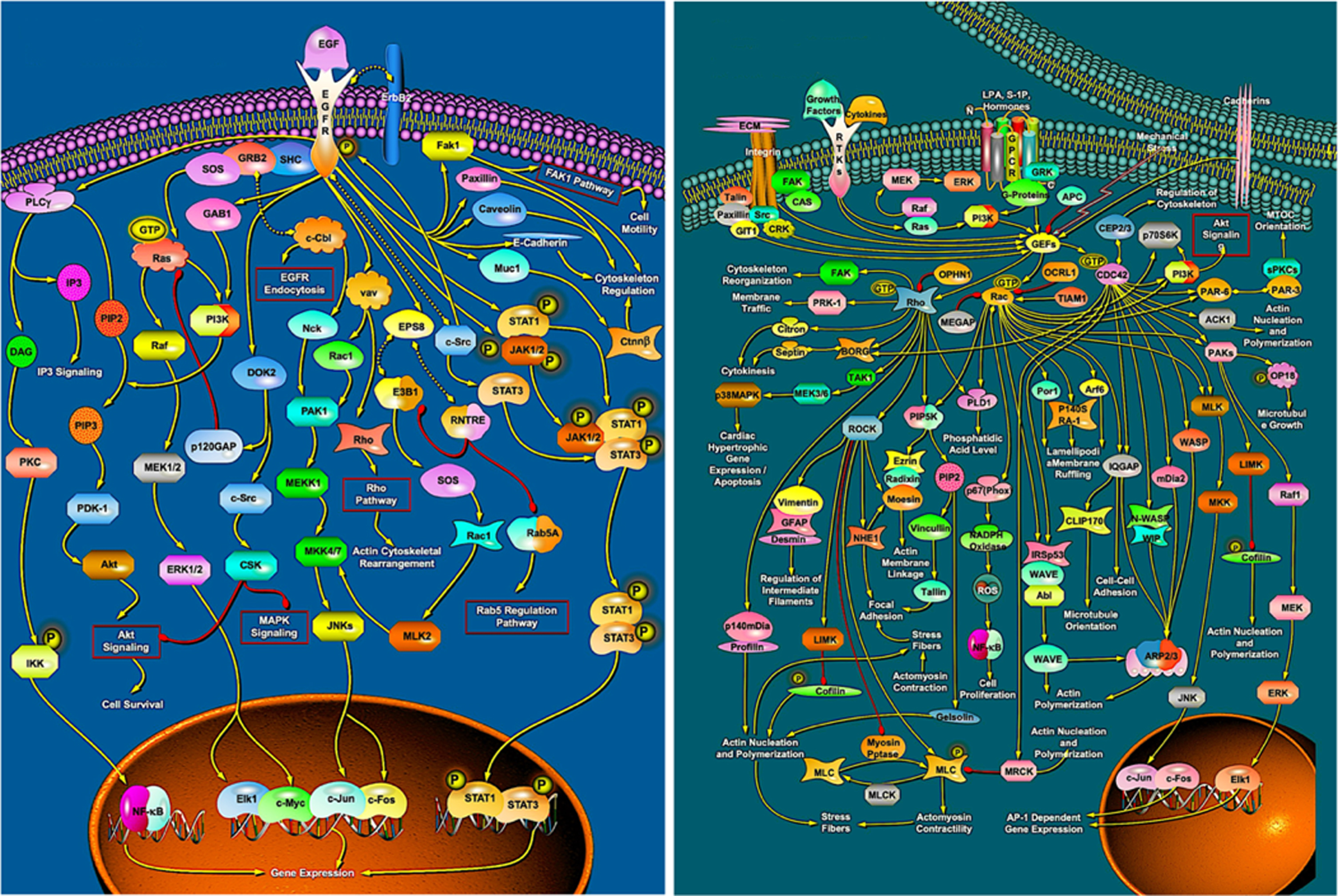
The basic principles of the development of complex organisms, whether animals or plants, are relatively straightforward [24, 30]. The fertilized egg divides and is then patterned by intrinsic lineage constraints and by a range of mainly short-range signalling interactions. Both may lead to a tissue changing its state, with the latter set of interactions also being able to generate a graded response. Cells generally respond to such instructions by activating protein networks (Fig. 4a) each of whose output is a process that leads to a change in phenotype [31]: they may undergo proliferation (mitosis), they can change their state (differentiation) and they can reorganise themselves through movement, shape change and tissue reorganisation (morphogenesis, Fig. 4b); they can also occasionally undergo programmed cell death (apoptosis). We know a fair amount about some of the signalling interactions and pathways used in the development of the main model organisms (e.g., mouse, Drosophila, C. elegans, zebrafish and Arabidopsis –see the ProteinLounge and KEGG websites) but much less about the process networks. Even where we know their protein constituents, it is hard to see how such networks operate because they are so complex, as Fig. 4 demonstrates.
Fig. 4
Protein networks that play important roles in animal development. a: The Epidermal growth factor (EGF) signalling pathway that often activates cell proliferation but has other roles. b: the Rho-GTPase network that directs morphogenesis through modulating cytoskeletal activity. The reasons why they should be so complicated are not known. (Courtesy of ProteinLounge, with permission).
In the context of evolutionary change, these networks fall into two categories. Changes that eventually lead to novel speciation are particularly driven by changes in tissue patterning, but also in differentiation, morphogenesis and apoptosis –these tend to operate relatively early in development [24]. Changes that lead to variants are primarily due to mutations that modify size and pigmentation –these generally occur in the later stages of development. The human species is a model system here: all human faces are patterned to have the same set of features and the differences across populations and individuals involve modifications in the local growth and in pigmentation networks.
Least understood and most important of these developmental networks are the signalling mechanism that pattern first the early embryo (e.g. the anterior-posterior body axis) and then its constituent tissues such as the vertebrate limbs [24]. More is known about several of the signal-response and process networks. Fig. 4a shows the EGF signalling network that activates mitosis. The input is the presence of a small protein, epidermal growth factor that binds to its receptor; the output is the activation of transcription factors that in turn initiate activity in the mitotic pathway. We have little idea why the EGF network needs to be so complicated although progress is being made on how this network operates [e.g. 32]. The situation is similar in the rho-GTPase network (Fig. 4b) which directs activity within the cytoskeleton and so mediates many of the morphogenetic events that underpin developmental anatomy [e.g. 33].
5.2The effects of mutation on protein networks
Understanding how mutations affect the phenotype of an organism first requires that we appreciate the details of the protein networks whose outputs drive its anatomical development, metabolism and physiological activity. Full analysis of these networks requires understanding the individual protein-protein interactions and the flow of smaller molecules within them. Only when we have a detailed grasp of these can we start to consider the possible effects of mutations that typically modify protein structure and hence their interactions with other proteins and with substrates, so modifying network outputs. This is a difficult but important area of work that is now attracting considerable attention from systems biologists [see [34–36] for reviews). What follows here is a summary of some of the key contemporary approaches and it is worth pointing out that much of the work in this important area is concerned with understanding mutations which lead to diseased states such as cancer rather than those that improve fitness [37].
In the context of novel speciation, we are primarily concerned with mutations that lead to anatomical modifications, and here it is worth pointing out that the options for a successful mutation in the protein networks that drive such change are limited [31]. Many, such as those for differentiation and apoptosis, have outputs that are essentially switches between states. Mutations in these networks are only likely to be successful if the resultant switching is selectable (e.g. [31, 38]). In such cases, the mutation as likely to affect network activation or inhibition as much as its internal dynamics. The developmental mutations most likely to be involved in future speciation are however those in networks involved in tissue patterning [24, 31]. Examples include the production of antero-posterior organisation (i.e. the Hox coding system), the production of a novel bone, changes in tooth morphology and the generation of a new pigment pattern in skin ectoderm.
Here, it is worth noting that developmental networks as a whole (e.g. Fig. 4a,b) seem surprisingly complicated for producing what can be seen as relatively straightforward outputs. One reason for this could be that have evolved to include a fair amount of buffering against the effects of mutation [39], and it may be for this reason that they are conserved to a considerable effect across the animal phyla [see the KEGG database [40]).
It is always possible, in principle at least, to describe networks as a graph of nodes and edges whose dynamics are given by a set of coupled differential equations. A first step in their analysis is to identify the key nodes and an obvious simplification is that all fast reactions will run at equilibrium, with the many slower reactions governing the overall dynamics of the system; however, such is this number that there is unlikely to be a key rate-limiting step. That said, such fast and slow reactions may be hard to identify, while mutations may well change the situation. Moreover, such can be the complexity of these networks that they may contain local domains that represent internal alternative routes through the network. It is currently extremely difficult to work out the full details of how these pathways work and harder still to estimate their dynamic properties. Although it is not yet possible to model in detail the full set of differential equations needed to model the complex protein network shown in Fig. 4a,b, considerable progress is being made, particularly in the study of signalling pathways [e.g. [41]).
The easiest protein networks to investigate and analyse are those that drive metabolism because many can be studied in vitro, as any textbook of biochemistry demonstrates. This is particularly so for the metabolic networks of bacteria such as E. coli since the ability to follow metabolite concentrations in mass cultures allows dynamic variables to be measured. It is much harder to study these networks in eukaryotic organisms, even in simple fungi such as Saccharomyces cerevisiae. This is partly because the quantitative data are much harder to obtain, and partly because it can be hard to identify local interactions within networks. Considerable effort is now being invested in analysing these networks [42–44]. Overton et al. [34] have provided a computational methodology for identifying transcription-factor targets through analysis of protein-interaction databases. Berkhout et al. [45] have developed techniques for analysing such data and shown how networks optimise fitness, while Paulson et al. [46] have considered how inferences may be made about parameter values. Of particular interest here are maximum entropy methods [47] which use statistical models to determine the most likely value of internal network parameters.
In the context of considering evolutionary change during development, a uniquely helpful system has been that of the 2D patterns generated by reaction-diffusion (Turing) kinetics, which essentially produce patterns of high concentration spots on a low concentration background ([48], for review, see [49]). For linear models, small changes in parameters, boundary conditions and timing (i.e. the sorts of changes that can be generated by mutation) can modulate spacing and pattern details (Fig. 5 [50, 51]), while nonlinear models can generate most of the patterns seen in vertebrates from fish to zebras [52, 53]. It has also been suggested that 3D Turing patterns can generate the architecture of complex bone systems such as those in limbs [54]. Although experimental evidence to support pattern formation based on reaction-diffusion kinetics has been hard to obtain, no other mechanism has yet been found capable of generating this range of modulatable patterns.
Fig. 5
The effect of timing on the initiation of zebra striping patterns. 1: Three zebra species. a: Equus quagga burchelli has ∼26 stripes. b; E. zebra as ∼50 stripes. c: E. grevyi has ∼75 stripes. (a: Courtesy of Gusjr; published under a CC Attribution generic 2.0 license. b: Courtesy of Yathin S. Krishnappa; published under a CC Attribution share-alike 4.0 international license. c: Courtesy of Thivier; published under a CC Attribution share-alike 3.0 unported license.) 2a,b c: 3, 3.5 and 5 week horse embryos on which have been drawn stripes of 200um separation such as can be generated by reaction-diffusion kinetics. ai and aii: the effect of normal embryonic growth on stripes laid down at 3 weeks at 3,5 and 5 weeks. (From [51] with permission from John Wiley and sons).
![The effect of timing on the initiation of zebra striping patterns. 1: Three zebra species. a: Equus quagga burchelli has ∼26 stripes. b; E. zebra as ∼50 stripes. c: E. grevyi has ∼75 stripes. (a: Courtesy of Gusjr; published under a CC Attribution generic 2.0 license. b: Courtesy of Yathin S. Krishnappa; published under a CC Attribution share-alike 4.0 international license. c: Courtesy of Thivier; published under a CC Attribution share-alike 3.0 unported license.) 2a,b c: 3, 3.5 and 5 week horse embryos on which have been drawn stripes of 200um separation such as can be generated by reaction-diffusion kinetics. ai and aii: the effect of normal embryonic growth on stripes laid down at 3 weeks at 3,5 and 5 weeks. (From [51] with permission from John Wiley and sons).](https://content.iospress.com:443/media/isb/2023/15-1-2/isb-15-1-2-isb220253/isb-15-isb220253-g005.jpg)
An alternative approach that has been successful in a few cases has been to simplify the situation and to use computational logic rather than differential equations to model networks. The network is formalised as a graph whose nodes are on/off or fast/slow switches and whose edges are Boolean operators [55, 56]. Once the network has been modelled in this way, it is computationally straightforward to test all possible Boolean states and see which produce the expected normal output and how mutation (changes in nodes and edges) affects the output.
There are at least two examples of this approach. The first is the analysis of the Fanconi-anaemia/breast-cancer pathway by Rodríguez et al. [57]. They modelled this as a Boolean network that included checkpoint proteins and DNA repair pathways. Using this model, they were first able to simulate normal behaviour and then to explore the role of repair pathways though simulating mutations. The second, and more important in an evolutionary and developmental context, is the sex determination network for gonad development (GSDN). This determines whether the early human gonad will become a testis (the SRY gene is expressed) or an ovary (the WNT4/β-catenin pathway is activated). Ríos et al. [58] modelled 19 of the key components in the GSDN network as Boolean nodes, each of which could be in an on or an off state, that interacted through the logical operators AND, OR and NOT. The model had 19 nodes and 78 regulatory operations, most of which derived from experimentation, and > 5 million possible initial states. Running all of these alternative showed that there were two major fixed-point attractors (stable states) that reflected male and female gonad development and a minor attractor that reflected a failure to differentiate. Added confidence could be had in this approach because the system could be modified to change node properties, so modelling known mutations. In such cases, the simulations gave the expected abnormal phenotypes.
On this basis, Boolean networks can clearly be used to model switches that direct options such as change state of differentiation or undergo mitosis/apoptosis. It is less clear that they can model the graded responses seen in patterning and morphogenesis or even mitotic rate, which can vary by a factor of five across a developing limb [59]. To approach such problems, more sophisticated approaches are needed. Groß et al. [60] have reviewed the ways in which this can be done and suggested that a particularly useful approach is to use probabilistic rules rather than differential equations to model the interactions between the proteins in a network and demonstrate its use for the Wnt signalling system. An alternative approach is to partition networks using Bond graphs which integrate network dynamics with energy flows [61].
Further insights into network kinetics may come from the analysis of complex medical disorders. Garg et al. [37], for example, explored how drugs altered their properties of the gene-regulatory networks where mutation leads to cancer. Of particular interest here is their analysis of the way in which mutation altered the balance between proliferation and apoptosis. More recently, Béal et al. [62] have devised ways in which models of melanomas and colorectal cancers can be expanded to include experimental data and be tuned to specific sets of mutants.
What this diversity of approaches makes clear is that theoretical progress is being made in this most difficult area of molecular genetics. There is however a long way to go before we can begin to understand the full range of anatomical changes that can occur in response to mutation.
6Selection and the pathway to speciation
Phenotypic variation within a population is the raw material on which selection operates. For phenotypic changes to emerge within that population in a novel environment, appropriately adapted fertile variants have to become predominant. As discussed above (Box 1), this is only likely to occur in small, founder populations. The success of such variants is the key step to producing subspecies. The final step in the pathway to in novel speciation, however, is that such variants will fail to produce fertile hybrids with descendants of the original parent population. This section considers these two key steps.
6.1Founder populations
The first step in the formation of new species is the separation from its parent population of a small group with a random sub-pangenome (the complete set of genes and their alleles within a population) of the parent pangenome. This is not a rare event: for any population in a relatively well-defined area, small groups at the periphery are always trying to expand their territory [63, 64], as the example of ring species (Fig. 1) makes clear. Indeed, the dispersal of humans across the world reflects such events.
If this founder group finds itself in a novel environment, either some variants will survive and prosper under the new selection pressures [65, 66], or the whole founder group will die out. Genetic analysis shows that the former will have a disproportionately large number of phenotypic variants. First, there will be a loss of heterozygosity (the Wahlund effect) and, second, genetic drift plays an important role in producing populations that are genetically unbalanced offspring as compared to the parent population. A classic experiment demonstrates this: Rich et al. [67] studied 12 replicates of large (50 M + 50 F) and small (5M+5 F) populations of red flour beetles (Trastaneum castaneum), each of which initially had equal numbers of dominant reds and recessives blacks, with numbers maintained for each generation through random selection. Over time, all large populations increased the proportion of red phenotypes, eventually achieving the expected 3 : 1 ratio. In contrast, the genetics of the small populations was unpredictable to the extent that one ended up being completely black (Fig. 6), with the dominant red gene having been lost.
Fig. 6
The effect of genetic drift in 12 large (N = 100) and 12 small (N = 10) populations that originally had equal numbers of red flour beetles (Trastaneum castaneum) with the dominant b+ allele and black flour beetles with the recessive genes (b–/b–). There was much more variation in the smaller populations and no obvious convergence to the extent that, in one of the small populations, the dominant gene was lost and the whole population ended up black. (From [55], with permission from the Society for the study of evolution (John Wiley Press) and thanks to John Herron for the redrawn and coloured image.)
![The effect of genetic drift in 12 large (N = 100) and 12 small (N = 10) populations that originally had equal numbers of red flour beetles (Trastaneum castaneum) with the dominant b+ allele and black flour beetles with the recessive genes (b–/b–). There was much more variation in the smaller populations and no obvious convergence to the extent that, in one of the small populations, the dominant gene was lost and the whole population ended up black. (From [55], with permission from the Society for the study of evolution (John Wiley Press) and thanks to John Herron for the redrawn and coloured image.)](https://content.iospress.com:443/media/isb/2023/15-1-2/isb-15-1-2-isb220253/isb-15-isb220253-g006.jpg)
Genetic drift is important for another reason: because the small group has a diminished and asymmetric pangenome as compared with that of the large original population, unexpected gene combinations can occur with a much higher frequency than might be expected. The resultant phenotypic changes may have a strong selective value and so become established in the normal way. Alternatively, it may have no strong selective effect one way or another and the novel phenotype may become established by chance. A possible example here is variable lung morphology: humans have two lobes in the left and three in the right lung; mice have a single left lobe and four right lobes. There seems to be no obvious physiological explanation for this, and the differences are as likely to have arisen as a result of drift during their long period of separation as for any other reason.
Changes in the phenotypes within a founder group thus result from two very different forms of random process: its limited pangenome and the random effects of genetic drift. Together, these can lead to novel traits that will allow it group to survive and flourish. These events can in principle be modelled using stochastic methodologies provided that key aspects of the genetic or phenotypic data for a population are known [68]. This is however generally difficult, because we have no good molecular model for the genetic basis of the great majority of traits.
6.2Selection and the formation of subspecies
The formal theory of selection is part of evolutionary population genetics [12, 66]. Selection biases the results of random breeding and so affects allele distribution in future populations. It should be emphasised that selection operates only on phenotypic traits, with the key parameter for a particular trait in a particular environment being fitness. This is a measure of the reproductive success of an organism with a particular allele in producing fertile offspring. The fitness coefficient is known as w and the associated selection coefficient s is connected to w by the simple formula
Our practical understanding of fitness comes from experiments done under controlled conditions, mainly studying traits that breed true and that follow Mendelian laws. A classic and well-studied example is the relationship between malaria resistance and sickle-cell anaemia [69]. Analysis of population data shows that there are different traits associated with mutations in the β-globin protein: wild-type proteins afford an individual no protection from malaria, double mutations cause sickle-cell anaemia but protect against malaria; a single mutation substantially diminishes an individual’s chance of getting the disease but does not lead to anaemia. Such special cases where the theoretical modelling is straightforward are however rare and it can be difficult in practice to apply the theory of evolutionary population genetics for a range of reasons that include:
• The model only holds for random breeding in large populations. In small populations, where genetic drift is important. random breeding behaviour will lead to fluctuations in allele frequencies to the extent that recessives may come to dominate a population in the absence of strong negative selection (Fig. 5 [67]).
• Most traits do not breed true as they are underpinned by many rather just one or two genes (e.g. Fig. 4).
• Experimentation on selection normally studies how single traits emerge under controlled conditions. In the wild, selection operates on the whole organism with every trait contributing to its fitness. It is rarely possible to know enough about such environments to understand fitness fully or to obtain sufficient breeding data to estimate selection pressures or to partition fitness variance. These difficulties are now however being re-examined and recent work has begun to show how they can sometimes be overcome [70, 71].
• It is a mistake to assume that traits are under independent selection. Larger size, for example, entails consumption of more food and perhaps a loss of agility [65, 72]. Such interactions across traits add a further degree of complexity to fitness.
The complexity of fitness away from laboratory conditions means that formal modelling using the classical theory of evolutionary population genetics can only be done when selection primarily operates on one or at the most a few traits, provided that they can be seen as independent [73]. A further limitation is that such studies can generally only examine a change in allele distributions from one stable state to another when all other conditions (e.g. selection pressures) remain constant.
There is however an alternative approach to studying selection which is to simulate it using stochastic methods. This approach is known as evolutionary game theory and dates back to the 1973 work of Maynard Smith and Price [74]. In essence, a model is constructed that includes breeding behaviour associated with individuals that have a range of genetically defined traits, each of which has an associated fitness for the local environment. The model runs for a generation, and this results in a daughter population that will be slightly different from the parent one. This process is then repeated until an equilibrium population is reached, which will usually be one with a stable phenotype distribution [75]. Game theory provides a methodology for testing hypotheses and exploring the implications of possible breeding/trait/environment scenarios as well as demonstrating the process of change.
An oversimple but immediately accessible example of this approach is given by the Primer simulation of natural selection available on Youtube [72]: this models the competing implications of size, speed and food availability in a self-replicating population. It demonstrates that, even for this very simple case, not only are the implications unpredictable because of the trait interactions, but that the final stable state depends on the initial conditions. Complex systems turn out to have final states that are neither expected nor predictable.
Selection in the wild adds two further complications. First, we cannot assume that selection coefficients remain constant over the long periods of time required for novel speciation to occur, as both traits and the environment may change (one would expect more stability in aqueous than land environments). Second, these coefficients are generally impossible to determine with accuracy because the limited amounts of experimental data available have to be used both to calculate selection constants and to test their implications. Perhaps the best that one can do here is a series of simulations using different subsets of the data for constant calculation and for verification. This approach is of course similar to the jackknife resampling techniques once used to test the quality of molecular phylogenies [76].
In summary, one can use modelling to explore hypotheses about selection, but it is not generally possible to make predictions about it for reasons that go beyond the difficulty of obtaining data. These include the random genetic profile of founder populations, the lack of understanding of how such profiles result in a spectrum of traits and the lack of a good theory of selection for multiple and complex traits.
6.3Chromosomal changes and the formation of new species
Once separated and in different environments, parent and founder populations will become increasingly distinct to the extent that that they will eventually be recognised as anatomically different. A classic example here is the hundreds of anatomically distinct populations of cichlid fish in Lake Victoria that descended from an initial population of perhaps a few species that was probably present ∼300 ka [77]. Today, many of these species can still interbreed, albeit that hybrid fertility may be limited [78]. In general, however, relatively minor anatomical differences alone say little about whether two homologous populations are subspecies that can interbreed or are distinct species whose eggs, even if fertilised, are incapable of producing fertile adults. Successful breeding has both phenotypic and genetic aspects.
There are several bars to successful interbreeding between two related groups. The earliest to occur reflects visual or behavioural traits that lead to a lack of interest in cross-mating in animals [20, 78]. There are also a few incompatibility genes whose expression make intergroup breeding essentially sterile, although the reasons are not always clear [79–81]. The most common cause of species separation however is chromosome mismatching. Normal, large, diploid population include a range of chromosomal rearrangements such as translocations, inversions, duplications, joinings and splittings [82, 83], albeit that each is rare.
Over time, different sets of minor chromosomal changes slowly accumulate in the parent and founder populations. Initially, their cumulative effect is to reduce hybrid fertility, but, as their chromosomes become more different, non-disjunction between the germ cells of the two populations becomes more likely. At this stage, hybrids first become sterile and eventually fail to develop. Here, it is worth noting that the bar to mitosis being possible is much higher than that for meiosis as crossover during meiosis may lead to the loss of genetic material [84].
Three examples demonstrate this and indicate the time scale of the process. The lion and tiger clades separated > 10 Ma [85] but can still interbreed to produce female “liger” offspring that are fertile (male offspring are sterile; see [86]). The borderline between fertility and infertility in hybrids is shown by mules, the hybrid offspring of horses and donkeys, which separated ∼2 Ma: although the very great majority are sterile, the occasional fertile example has been recorded [17, 18]. The reason for the difference is, of course, that lions and tigers both have 19 pairs of chromosomes whereas horses and donkeys respectively have 32 and 31 pairs. Third, most of the diverse Canis genus that includes wolves, dogs, grey wolves, dingoes, coyotes and golden jackals can interbreed and produce fertile hybrids They all have 39 pairs of chromosomes and any minor differences are reproductively insignificant. Other members of the wider Canidae family, such as foxes, which separated off the main line > 10 Ma now have 34 main chromosomes and some additional small ones; they are thus unable to breed with members of the Canis genus [87].
The key to irreversible species separation in general is thus the accumulation of differences in chromosome organisation and number between the two populations. The initial formation and subsequent spread of such changes through a population is, as the examples given above demonstrate, rare, slow and stochastic. It is impossible to predict where changes to chromosome structure will occur because there are no constraints on these complex changes, neither are there any endpoints or equilibria. The structural differences continue to accumulate with there being no criteria for determining when numbers are sufficient to lead to non-disjunction. We just know that, given enough time, the accumulation of chromosomal differences will result in this happening.
7Discussion
Table 1 summarises the series of events that lead to the formation of a new species and Fig.1 shows the levels of scale at which they occur. One point is immediately striking: many of these events involve random activities. The processes of speciation as a whole can be seen as maximising opportunities for genetic variation, phenotypic variation and selection. Indeed, it is hard to envisage a richer approach to the creation of phenotypic novelty, selection and ultimately speciation. The extent of this variation has two obvious corollaries. Perhaps the most obvious is that, as speciation involves events from the genome to the climate, it is unlikely that it will ever be possible to produce an integrated model that describes the generation of new species. The other is that models at the events at particular levels will generally have to include stochastic elements.
Figure 3 makes a key point about the underlying morphology of modelling. Outputs from one level feed upwards as the raw material for change at the next higher level. Such is the complexity of the system, however, that events taking place at a single level often include feedback interactions from higher and lower levels. Examples are the complex effects of selection in the wild, which feed downwards to modulate events lower levels (e.g. environmental temperature determines gender in some reptiles [88]), and protein signals, which direct events at higher levels [24]. Modelling at a single level is always going to be difficult, particularly because we lack much of the numerical data that is required.
It is because the relevant data are so robust that the greatest successes in evolutionary biology have been in unravelling evolutionary history using methodologies that include molecular phylogenetics, cladistic analysis and coalescence analysis. This work, as mentioned earlier, has produced detailed phylogenies across the biosphere and so provided a theoretical context in which to embed the details of the fossil record. These methodologies, as applied to human mitochondrial DNA and other sequence data, have allowed us, for example, to discover details of the travels of H. sapiens over the past ∼65 Ky when early founder groups left Africa to populate the modern world (e.g. [89], for review, see [1]).
Indeed, there is now so much DNA data on individual species that the various technologies can identify likely sequences in earlier common ancestors within a clade. Such data ought, in principle, to tell us about the mutations that caused an ancestor species to give rise to two contemporary ones. In practice, however, this is very difficult, partly because we do not know which were the key genes mutation in which drove separation and partly because the sequence of mutational changes is not something that the methodologies predict. Given the long time needed for full speciation and the subsequent period for which that species has survived, it is hard even to identify the initial changes that drive diversification.
As mutation is essentially stochastic and occurs across the whole genome, with selection depending partly on fitness and partly on drift accompanied by neutral selection, it is also difficult to see how change can be modelled in any eukaryote organism. Even in viruses, the simplest of organisms, it is still not easy to identify the likely future harmful mutations protection against which require new annual influenza vaccines [7].
The classic success in the modelling of evolutionary change has been, of course, evolutionary population genetics, which aims to quantify events from mutation change to the emergence of novel phenotypes. The core elements of this theory were in place by the 1960 s, before the DNA revolution had clarified the molecular basis of evolutionary change. Nevertheless, its models on how mutations move through a population and the special properties of founder groups still hold good. Its modelling of phenotypic change is however very thin for two reasons: first, it is hard to model selection except under laboratory conditions (for an exception, see [64] and below), second, its model of traits and features is oversimplified. The theory supposes, on the basis of Mendel’s work, that traits and their variants were based on very few genes and their allele alternatives. This is so for individual proteins and a few macroscopic traits that depend on so-called Mendelian genes, but not for most eukaryotic traits, which are underpinned by the activities of complex protein networks (e.g. Fig. 4a,b).
While it is possible to unpick some of the features of these networks through our understanding of protein function, it has proven very much harder to model their normal activity or to investigate how this activity might be modified by mutation. Nevertheless, as the work described in Section 5.2 makes clear, the use of a wide variety of modelling approaches has allowed some progress to be made in this most difficult of areas. It will be interesting to see which approaches will be most helpful over the next few years and the sorts of prediction that might emerge from this work. Many will be straightforward, but complex systems can have a range of outputs with the most intriguing being unpredictable emergent properties (Table 1): these arise when the complex interactions at one level produce an unexpected output that affects events at a higher level of scale (Fig. 3). In the context of evolutionary change, there are two obvious examples. The simpler one arises from the distribution of alleles in founder populations: one expects more recessive heterozygotes to form, but one cannot predict which ones or what their cumulative effect will be in the phenotype. The second is more complex and arises from the effects of unexpected allele combinations on the protein networks whose outputs particularly affect developmental anatomy and physiology [22, 23].
Perhaps, however, the key step in novel speciation is the formation of founder groups of small numbers of individuals that find themselves in new habitats with novel selection pressures. The particular sets of genetic properties associated with such groups (Box 1) encourage the emergence of rare and even unexpected traits. While it possible to study some of the events experimentally using strong selection pressures on groups of organisms from standard species such as Drosophila, modelling the process is far harder [20, 21].
Interesting insights into the emerging properties of small groups of individuals in long-isolated groups may well come from the most interesting species in the study of evolution –humans. Not only do we have vast amounts of mutation data on H. sapiens, which is available for gene-wide association studies (GWAS) into quantitative traits [90], but there are still a few long-isolated human tribes, such as those in the Amazonian rain forests [91]. It will be interesting to see if any novel traits have emerged in these tribes since they separated away from their original founder population, which migrated from North to South America some 10.5 Ka, or more than 200 generations ago, although they are now becoming less isolated [92]. Even here, it will be difficult to mesh any such traits with the selection pressure to which generations of these groups were subjected given that they could well be the results of genetic drift.
Another facet of the process of speciation that is extremely hard to model is selection in the wild. Evolutionary population genetics focuses on the effects of one or perhaps two selection pressures on a single trait. It does this partly because the theory is tractable and partly because making numerical predictions requires numerical constants. Fitness estimation is difficult, although new methods are now available [e.g. [70]). Even here, this model of selection is oversimplified because the process of selection involves every aspect of an organism’s surrounding. These include food availability, support from symbionts, predation, habitat availability and the effects of climate; it is hard to imagine that each remains static for long periods needed for novel speciation except perhaps under marine situations. Modelling all of this is only practical using game theory and perhaps there is more that can be done here.
There are however still two aspects of speciation where detailed modelling is particularly hard, even within a known founder group. The first is the genetic changes that occur from generation to generation, which has three random components: the location of the few new mutations (~64 of the 3 billion bp in the human genome [93]), the location of the cross-over sites that form during meiosis and the effects of choice of non-incestuous breeding partners. The second is the locations of the chromosomal alterations that are the final step in species separation; their occurrence is very rare, and it is worth noting that, even after several million generations of separation [85], the chromosomal differences between lions and tigers are not sufficient to block the formation of fertile hybrids.
In conclusion, this paper has considered the various aspects of modelling the events that lead to speciation and has pointed to some successes. There is however still a long way to go, with the major challenge being to model its various random events. In principle, this is very difficult but, in practice, it may prove less hard than expected in cases where the number of possible outcomes is found to be limited and for which we have fitness criteria.
Acknowledgment
I thank Gillian Morriss-Kay for commenting on the manuscript and an anonymous referee for helpful criticisms and pointers on the analysis of protein networks.
References
[1] | Bard J. Evolution: The Origins and Mechanisms of Diversity, CRC Press, (2022) . |
[2] | Coyne J.A. , Orr H.A. , Speciation. Sinauer Press, Oxford, (2004) . |
[3] | Gould S.J. A Tree Grows in Paris: Lamarck’s Division of Worms and Revision of Nature, In: The Lying Stones of Marrakech: Penultimate Reflections in Natural History, Harmony Books, (2000) , pp. 115–143. |
[4] | Gehring W.J. , The evolution of vision, Wiley Interdiscip Rev Dev Biol 3: ((2014) ), 1–40. |
[5] | Kemp T. The Origin of Higher Taxa: Palaeobiological, Developmental, and Ecological Perspectives, University of Chicago Press, (2015) . |
[6] | Wood B. Human evolution: a very short introduction, Oxford University Press Oxford, (2019) . |
[7] | Agor J.K. and Özaltın O.Y. , Models for predicting the evolution of influenza to inform vaccine strain selection, Hum Vaccin Immunother 14: ((2018) ), 678–683. |
[8] | Darwin C.R. , Extract from an unpublished Work on Species, by C. Darwin, Esq., consisting of a portion of a Chapter entitled, “On the Variation of Organic Beings in a state of Nature; on the Natural Means of Selection; on the Comparison of Domestic Races and true Species.” Proc Linn Soc 3: ((1858) ), 46–53. Wallace A. , On the tendency of varieties to depart indefinitely from the original type, Proc Linn Soc 3: ((1858) ), 53–62. https://darwin-online.org.uk/converted/pdf/1858_species_F350.pdf |
[9] | Darwin C.R. On the Origin of Species by Means of Natural Selection or the Preservation of Favoured Races in the Struggle for Life, John Murray, London, (1959) . |
[10] | Irwin D.E. , Irwin J.H. and Price T.D. , Ring species as bridges between microevolution and speciation, Genetica, (2001) ;112–113:223–243. |
[11] | Mendel G. Experiments in plant hybridization, 1866. English translation: https://www.esp.org/foundations/genetics/classical/gm-65.pdf |
[12] | Fisher R.A. The Genetical Theory of Natural Selection, Oxford Clarendon Press, (1930) . |
[13] | https://en.wikipedia.org/wiki/Modern_synthesis_(20th_century). |
[14] | Rosenberg N.A. and Nordborg M. , Genealogical trees, coalescent theory and the analysis of genetic polymorphisms, Nat Rev Genet 3: ((2002) ), 380–390. |
[15] | LaBar T. and Adami C. , Evolution of drift robustness in small populations, Nat Commun 8: ((2017) ), 1012. |
[16] | Orlando L. , et al., Revising the recent evolutionary history of equids using ancient DNA, Proc Natl Acad Sci U S A 106: ((2009) ), 21754–21759. |
[17] | Ryder O.A. , Chemnick L.G. , Bowling A.T. , and Benirschke K , Male mule foal qualifies as the offspring of a female mule and jack donkey, JHered 76: ((1985) ), 379–81. |
[18] | Rong R. , et al., A fertile mule and hinny in China, Cytogenet Cell Genet 47: ((1988) ), 134–139. |
[19] | Skinner M.K. and Nilsson E.E. , Role of environmentally induced epigenetic transgenerational inheritance in evolutionary biology: Unified Evolution Theory, Environ Epigenet 7: ((2021) ), dvab012. |
[20] | Rice W.R. and Salt G.W. , The evolution of reproductive isolation asa correlated character under sympatric conditions: experimental evidence, Evolution 44: ((1990) ), 1140–1152. |
[21] | Waddington C.H. , Genetic assimilation, Adv Genet , 10: ((1961) ), 257–293. |
[22] | Hastings M.H. , Smyllie N.J. and Patton A.P. , Molecular-genetic Manipulation of the Suprachiasmatic Nucleus Circadian Clock, J Mol Biol 432: ((2020) ), 3639–3660. |
[23] | Janzen E. , et al., Emergent properties as by-products of prebiotic evolution of aminoacylation ribozymes, Nat Commun 12: ((2022) ), 3631. |
[24] | Barresi M. , Gilbert S.F. Developmental Biology (12th edition), Oxford University Press, (2019) . |
[25] | Gilbert S.F. , Bosch T.C. and Ledón-Rettig C. , Eco-Evo-Devo: developmental symbiosis and developmental plasticity as evolutionary agents, Nat Rev Genet 16: ((2015) ), 611–622. |
[26] | Nachman M.W. and Crowell S.L. , Estimate of the mutation rate per nucleotide in humans, Genetics 156: ((2000) ), 297–304. |
[27] | Reid J.B. and Ross J.J. , Mendel’s genes: toward a full molecular characterization, Genetics 189: ((2011) ), 3–10. |
[28] | Giam C.Z. , Hayashi S. and Wu H.C. , Characterization of a novel lipoprotein mutant in Escherichia coli, J Biol Chem 10: ((1984) ), 5601–5605. |
[29] | Pavlopoulos A. and Akam M. , Hox gene Ultrabithorax regulatesdistinct sets of target genes at successive stages of haltere morphogenesis, Proc Natl Acad Sci U S A, Drosophila 108: ((2011) ), 2855–2860. |
[30] | Bard J. , A systems biology representation of developmental anatomy, J Anat 218: ((2011) ), 591–599. |
[31] | Bard J. , Driving developmental and evolutionary change: A systems biology view, Prog Biophys Mol Biol 11: ((2013) ), 83–91. |
[32] | Koseska A. and Bastiaens P.H. , Processing Temporal Growth Factor Patterns by an Epidermal Growth Factor Receptor Network Dynamically Established in Space, Annu Rev Cell Dev Biol 36: ((2020) ), 359–383. |
[33] | Nguyen L.K. , Kholodenko B.N. and von A. , Kriegsheim, Rac1 and RhoA: Networks, loops and bistability, Small GTPases 9: ((2018) ), 316–321. |
[34] | Overton I.M. , et al., Functional Transcription Factor Target Networks Illuminate Control of Epithelial Remodelling, Cancers (Basel) 12: ((2020) ), 2823. |
[35] | Koutrouli M. , Karatzas E. , Paez-Espino D. and Pavlopoulos G.A. , A Guide to Conquer the Biological Network Era Using Graph Theory, Front Bioeng Biotechnol 8: ((2020) ), 1–26. |
[36] | Tan A.-K. , Huang P.H. ((2017) , Editors) Kinase Signaling Networks, Springer: Humana Press. |
[37] | Garg A. , et al., Efficient computation of minimal perturbation sets in gene regulatory networks, Front Physiol 4: ((2013) ), 361.1–361.10. |
[38] | Gañan Y. , Macias D. and Basco R.D. , Morphological diversity ofthe avian foot is related with the pattern of msx gene expression inthe developing autopod,, Dev Biol 196: ((1998) ), 33–41. |
[39] | Barbaric I. , Miller G. and Dear T.N. , Appearances can be deceiving: phenotypes of knockout mice, Brief Funct Genomic Proteomic 6: ((2007) ), 91–103. |
[40] | Kanehisa M. , Toward understanding the origin and evolution of cellular organisms, Protein Sci 28: ((2019) ), 1947–1951. |
[41] | Fey D. , Aksamitiene E. , Kiyatkin A. and Kholodenko B.N. , Modeling of Receptor Tyrosine Kinase Signaling: Computational and Experimental Protocols, Methods Mol Biol 1636: ((2017) ), 417–453. |
[42] | Omranian S. , Nikoloski Z. and Grimm D.G. , Computational identification of protein complexes from network interactions: Present state, challenges, and the way forward, Comput Struct Biotechnol J 20: ((2022) ), 2699–2712. |
[43] | Huang L. , Liao L. and Wu C.H. , Evolutionary Model Selection and Parameter Estimation for Protein-Protein Interaction Network Based on Differential Evolution Algorithm, IEEE/ACM Trans Comput Biol Bioinform 12: ((2015) ), 622–631. |
[44] | Lillacci G. and Khammash M. , Parameter estimation and model selection in computational biology, PLoS Comput Biol 6: ((2010) ), e1000696. |
[45] | Berkhout J. , et al., How biochemical constraints of cellular growth shape evolutionary adaptations in metabolism, Genetics 194: ((2013) ), 505–512. |
[46] | Paulson J.A. , Martin-Casas M. and Mesbah A. , Fast uncertainty quantification for dynamic flux balance analysis using non-smooth polynomial chaos expansions, PLoS Comput. Biol 15: ((2019) ), e1007308. |
[47] | De Martino A. and De Martino, D. , An introduction to the maximum entropy approach and its application to inference problems in biology, Heliyon ((2018) ), e00596. |
[48] | Turing A.M. , The chemical basis of morphogenesis, Philos Trans R Soc B 237: ((1952) ), 37–72. |
[49] | Lacalli T.C. , Patterning, from conifers to consciousness: Turing’s theory and order from fluctuations, 10:, Front Cell Dev Biol 10: ((2022) ), 871950. |
[50] | Bard J. and Lauder I. , How well does Turing’s theory of morphogenesis work? J Theor Biol 45: ((1974) ), 501–531. |
[51] | Bard J.B.L. , A unity underlying the different zebra striping patterns, J Zoology 183: ((1977) ), 527–539. |
[52] | Bard J.B.L. , A model generating aspects of zebra and other mammalian coat patterns, J Theor Biol 93: ((1981) ), 363–385. |
[53] | Barrio R.A. , et al., A two-dimensional numerical study of spatial pattern formation in interacting Turing systems, Bull Math Biol 61: ((1999) ), 483–505. |
[54] | Stewart T.A. , Bhat R. and Newman S.A. , The evolutionary origin of digit patterning, Evodevo 21: ((2017) ), 8:21. |
[55] | Schwab J.D. , et al., Reconstructing Boolean network ensembles from single-cell data for unraveling dynamics in the aging of human hematopoietic stem cells, Comput Struct Biotechnol J 19: ((2021) ), 5321–5332. |
[56] | Stöcker B.K. , Köster J. , Zamir E. and Rahmann S. , Modeling and simulating networks of interdependent protein interactions, Integr Biol (Camb) 10: ((2018) ), 290–305. |
[57] | Rodríguez A. , et al., A Boolean network model of the FA/BRCA pathway, Bioinformatics 28: ((2012) ), 858–866. |
[58] | Ríos O. , et al., A Boolean network model of human gonadal sex determination, Theor Biol Med Model 16: ((2015) ), 12–26. |
[59] | Hornbruch A. and Wolpert L. , Cell division in the early growth and morphogenesis of the chick limb, Nature 226: ((1970) ), 764–766. |
[60] | Groß A. , et al., Representing dynamic biological networks with multi-scale probabilistic models, Commun. Biol 2:21: ((2019) ), 1–12. |
[61] | Pan M. , et al., Modular assembly of dynamic models in systems biology, PLoS Comput Biol 17: ((2021) ), e1009513. |
[62] | Béal J. , et al., Personalized logical models to investigatecancer response to BRAF treatments in melanomas and colorectal cancers, PLoS Comput Biol 17: ((2021) ), e1007900. |
[63] | Templeton A.R. , The reality and importance of founder speciation in evolution, Bioessays 30: ((2008) ), 470–479. |
[64] | Vucetich J.A. and Waite T.A. , Spatial patterns of demography and genetic processes across the species’ range: Null hypotheses for landscape conservation Genetics, Conservation Genetics 4: ((2003) ), 639–645. |
[65] | Brooks J. and Yamamoto S. , The founder sociality hypothesis, Ecol Evol 11: ((2021) ), 14392–14404. |
[66] | Saetre G-P and Ravinet M. , Evolutionary Genetics: Concepts, Analysis, and Practice, Oxford University Press. Oxford, (2019) . |
[67] | Rich S.S. , Bell A.E. and Wilson S.P. , Genetic drift in small populations of Tribolium, Evolution 33: ((1979) ), 579–584. |
[68] | Koehl A.J. and Long J.C. , The contributions of admixture and genetic drift to diversity among post-contact populations in the Americas, Am J Phys Anthropol 165: ((2018) ), 256–268. |
[69] | Williams T.N. and Thein S.L. , Sickle Cell Anemia and Its Phenotypes, Annu Rev Genomics Hum Genet 19: ((2018) ), 113–147. |
[70] | Haasdijk E. and Heinerman J. , Quantifying Selection Pressure, Evol Comput 26: ((2018) ), 213–235. |
[71] | Rose K.E. , Rees M. and Grubb P.J. , Evolution in the real world: stochastic variation and the determinants of fitness in Carlina vulgaris, Evolution 56: ((2002) ), 1416–1430. |
[72] | Primer simulation of natural selection: www.youtube.com/watch?v=0ZGbIKd0XrM |
[73] | Gorrell J.C. , et al., Adopting kin enhances inclusive fitness in a social red squirrels, Nat Commun 1: ((2010) ), 1–4. |
[74] | Maynard Smith J. and Price G.R. The Logic of Animal Conflict, Nature 246: ((1973) ), 15–18. |
[75] | Nowak M.A. , Tarnita C.E. and Antal T. , Evolutionary dynamics in structured populations, Philos Trans R Soc Lond B Biol Sci 365: ((2010) ), 19–30. |
[76] | Henderson A.R. , The bootstrap: a technique for data-driven statistics, Using computer-intensive analyses to explore experimental data, Clin Chim Acta 359: ((2005) ), 1–26. |
[77] | Schedel D.D.B. , Musilova Z. and Schliewen U.K. , East African cichlid lineages (Teleostei: Cichlidae) might be older than their ancient host lakes: new divergence estimates for the east African cichlid radiation, BMC Evol Biol 19:94: ((2019) ), 1–25. |
[78] | Stelkens R.B. , Schmid C. and Seehausen O. , Hybrid breakdown in cichlid fish, PLoS One 10: ((2015) ), e0127207. |
[79] | Davies B. , et al., Re-engineering the zinc fingers of PRDM9 reverses hybrid sterility in mice, Nature 530: ((2016) ), 171–176. |
[80] | Maheshwari S. and Barbash D.A. , The genetics of hybrid incompatibilities, Ann Rev Genet 45: ((2011) ), 331–355. |
[81] | Rieseberg L.H. and Blackman B.K. , Speciation genes in plants, Ann Bot 106: ((2010) ), 439–455. |
[82] | Jacobs P.A. , et al., Estimates of the frequency of chromosomeabnormalities detectable in unselected newborns using moderatelevels of banding, J Med Genet 9: ((1992) ), 103–108. |
[83] | Fan H.T. , et al., Structural chromosomal abnormalities in couples in cases of recurrent spontaneous abortions in Jilin Province, China, Genet Mol Res 15: ((2016) ), 1–7. |
[84] | O’Connor C. , Human chromosome translocations and cancer, Nature Education 1: ((2008) ), 56. |
[85] | Tseng Z.J. , et al., Himalayan fossils of the oldest known pantherineestablish ancient origin of big cats, Proc Biol Sci 28: ((2013) ), 20132686. |
[86] | |
[87] | Wayne R.K. , Nash W.G. and O’Brien S.J. , Chromosomal evolution of the Canidae, I. Species with high diploid numbers, Cytogenet Cell Genet 44: ((1987) ), 123–133. |
[88] | Merchant-Larios H. , Díaz-Hernández V. and Cortez D. , Molecular and Cellular Mechanisms Underlying Temperature-Dependent Sex Determination in Turtles, Sex Dev 15: ((2021) ), 38–46. |
[89] | Ioannidis A.G. , et al., Paths and timings of the peopling of Polynesia inferred from genomic networks, Nature 597: ((2021) ), 522–526. |
[90] | Lee J. , et al., Variable Selection and Joint Estimation of Mean and Covariance Models with an Application to eQTL Data, Comput Math Methods Med 2018: ((2018) ), 4626307. |
[91] | Salgado S. Amazônia, Taschen Press, (2021) . |
[92] | Brandini S. , et al., The Paleo-Indian Entry into South America According to Mitogenomes, Mol Biol Evol 35: ((2018) ), 299–311. |
[93] | Drake J.W. , et al., Rates of spontaneous mutation, Genetics 148: ((1998) ), 1667–1686. |

