Reverse engineering of a mechanistic model of gene expression using metastability and temporal dynamics

2.1Mechanistic model

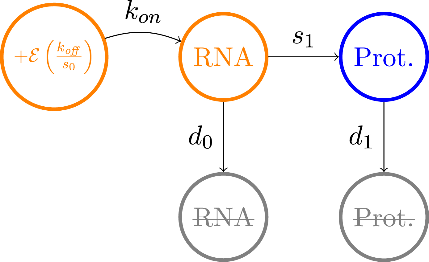
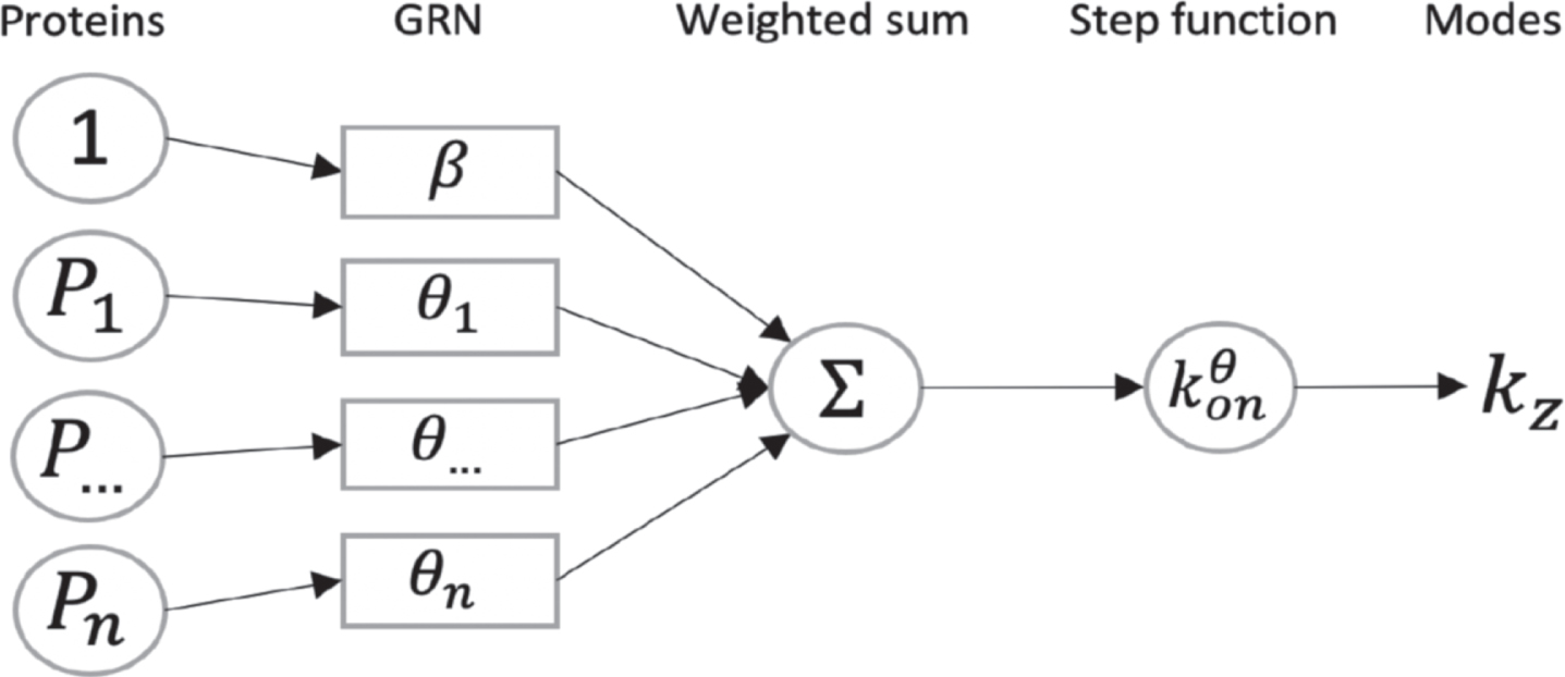
The model which is used throughout this article has been introduced in [16]. It is based on a hybrid version of the well-established two-state model of gene expression [21, 38], where a gene is described by the state of a promoter, which can be {on, off}. If the promoter is on, mRNAs are transcribed at a rate s₀, which are then translated into proteins at a rate s₁. Degradation of both mRNAs and proteins occurs respectively at a rate d₀ and d₁. The transitions between the states on and off occur at exponential times of rates k_on and k_off. We consider the so-called bursty regime of this model, when k_on ⪡ k_off, which corresponds to the experimentally observed situation where active periods are short but characterised by a high transcription rate, thereby generating bursts of mRNA [34, 43, 50]. We describe the random times at which these bursts occur by an exponential law of parameter k_on, and their random intensity by an exponential law of parameter k_off/s₀ (see Figure 1). This model is compatible with real single-cell data, as mRNAs quantity at the steady state follows a Gamma distribution, which is known to describe accurately continuous single-cell data [2].

Fig. 1

Approximation of the two-states model of gene expression in the bursty regime.

Neglecting the molecular noise associated to mRNA and protein quantities, we obtain the following mathematical description of the model:

We point out that assuming that this model is able to reproduce real single-cell datasets, we make the underlying hypothesis, which is implicit in most GRN inference methods, that, contrary to its state, the GRN structure is not modified under the action of some hidden variables. One should not that our interaction model is an approximation of the underlying biochemical cascade reactions, and that the genes we modeled need not to be transcription factors. This is possible thanks to the use of our mechanistic model which integrates the notion of timescale separation [16]. It assumes that every biochemical reaction such as metabolic changes, nuclear translocations or post-translational modifications are faster than gene expression dynamics and that they can be abstracted in the interaction between 2 genes [5]. To explicitly model slow changes like some epigenetic changes by allowing the structure of the GRN to change during differentiation, would definitely add realism but at the cost of a much higher complexity: the number of additional unobserved parameters would dramatically increase the problems of identifiability, making a reverse-engineering method out of reach.

2.2Simplification in the fast transcription regime

In line with several experiments [2, 22], we consider that mRNA bursts are fast in regard to protein dynamics, i.e d_0,i ⪢ d_1,i with k1,id0,i fixed. The correlation between mRNAs and proteins produced by a gene i is then very small, and the model can be reduced by removing mRNA and making proteins directly depend on the burst. We obtain a simplified network model in which only proteins are described:

2.3Metastability and reduction

We now perform a reduction of the model 3 into a coarse-grained model on a limited number of metastable basins, providing an approximate landscape of the differentiation process. For this sake, we introduce a typical time scale k¯ for the rates of promoters activation kon,iθ , and a typical time scale d¯ for the rates of proteins degradation. Then, we define the scaling factor ɛ=d¯k¯ which characterizes the difference in dynamics between two processes: 1. gene bursting dynamics and 2. protein dynamics. It is generally considered that promoter switches are fast with respect to protein dynamics, i.e that ɛ ⪡ 1, at least for eukaryotes [48].

In that context, we can approximate the conditional expectation of the bursts of proteins associated to a gene i knowing the proteins vector P, that we denote ρ_i (P), by its quasistationary approximation ρi¯(P)=kon,iθ(P)ci . The model (3) can therefore be coarsely approximated by a system of ordinary differential equations:

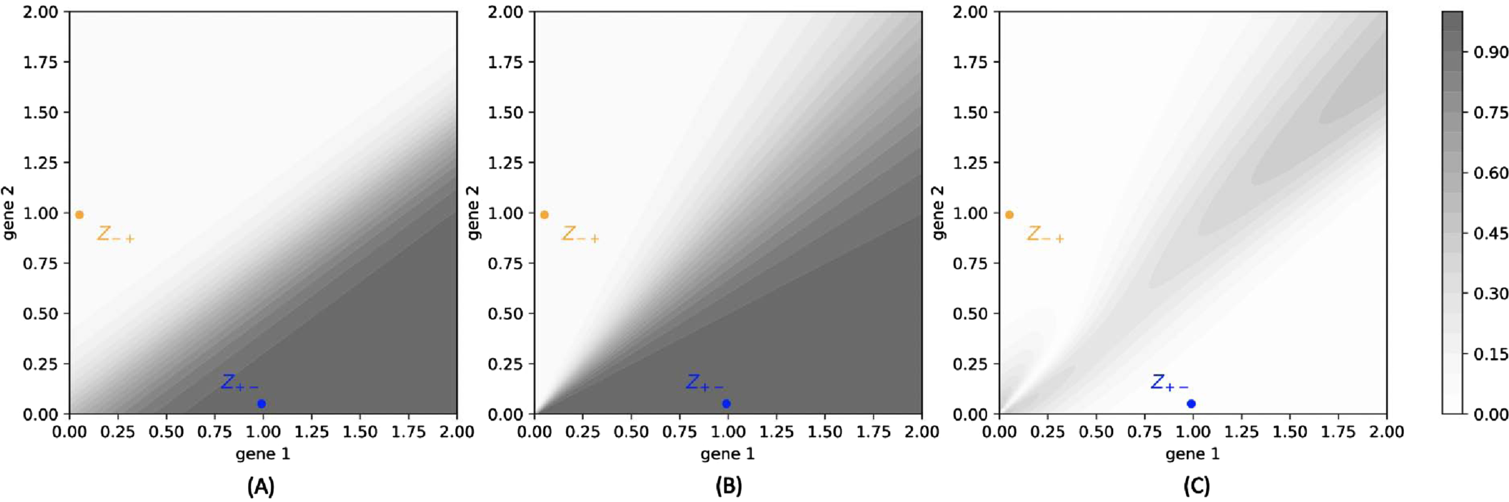
Assuming that the dynamical system (4) has no limit cycles or more complicated orbits, the gene expression space can be then decomposed in a set of basins of attraction Z = {Z₁, ⋯ , Z_m}, respectively associated to m stable solutions of:

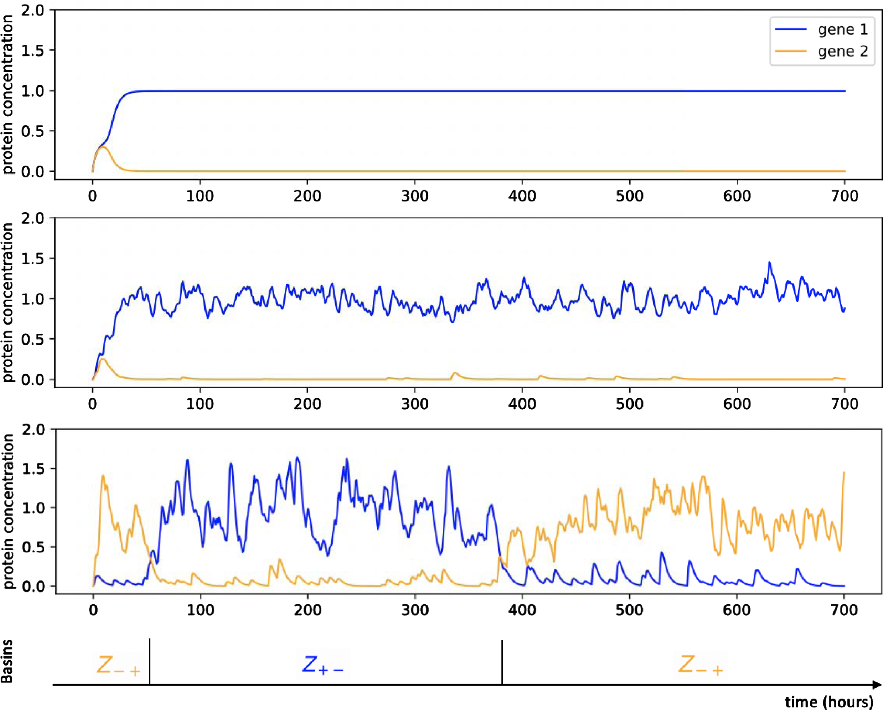
Fig. 2

Example of trajectories associated to the symmetric toggle-switch network described in Table 1, for different values of ɛ: from top to bottom, ɛ = 0, ɛ = 1/50 and ɛ = 1/10. For ɛ = 1/10, we observe stochastic transitions between the two metastable basins denoted Z_+- and8 Z_-+.

Adopting the paradigm of metastability referred in the introduction, we identify the basins of attraction associated to the equilibrium of the deterministic system (4) to cell types [18]. A cell type then corresponds to a metastable sub-region of the gene expression space, and the process can be coarsely reduced to a new (Markovian) discrete process on the cell types. These cell types represent the potential wells in the developmental landscape of differentiation associated to the model (3) [49], the centers of which are the attractors solutions of the system (5). To characterize more precisely the landscape, it would remain to describe:

Point 1. corresponds to the transition rates of the coarse-grained model on the cell types, which are known to be very difficult to link analytically to a GRN [51]. They generally depends on the values of the stationary distribution uˆθ of proteins on the saddle point of the system (4), which are located on areas of the gene expression space where the probability to find a cell is weak. As discussed in Section 7.2 with more details, this feature does not seem to be exploitable in the context of GRN inference. Point 2. can be described by the behaviour of the potential function Vθ=-ln(uˆθ)) in the neighborhood of the attractors. This feature seems more accessible because cells are likely to be measured around the attractors in the gene expression space. We are now going to develop an heuristic reasoning for approximating the function uˆθ when the bursts rate functions are of the form (2).

3.1Mixture approximation of the proteins distribution

On one side, the transitions of the coarse-grained model described in Section 2.3 happen at a time scale which is expected to be of the order of eCɛ , where C is an unknown constant depending on the basins (owing to a Large deviations principle studied in [51]). For small ɛ, such transitions are then generally rare events, and it can be considered that the process spends in each basin a time long enough to equilibrate inside, i.e that a cell reaches between each transition its quasistationary distribution within a basin. On the other side, the sigmoidal form (2) for the functions kon,iθ implies that these functions must not vary significantly within a basin: a rough approximation could lead to identify the bursts rate in each basin by its dominant rate inside, corresponding to the value of the function k_on,i on the attractor P_z. For any gene i = 1, ⋯ , n and any basin z ∈ Z, we can then approximate:

Finally, we can approximate the stationary distribution of the process associated to a given GRN uˆθ by a mixture of Gamma distributions. Denoting for any z∈Z,i=1,⋯,n,kz,i=kon,iθ(Pz) , we obtain

The heuristic analysis presented above then states that when the functions k_on,i are close to constant functions inside the basins and that the scaling factor ɛ is small, the mixture approximation (6) is a good approximation of the distribution uˆθ . We remark that this is straightforward when the scaling factor ɛ is close to 0. Indeed, any GRN θ is associated for any value of ɛ to an unknown stationary distribution, that we denote uˆɛθ , which converges to a sum of Dirac on the attractors when ɛ → 0 [36]. Then we see that the Gamma mixture uˆɛ associated to the same ɛ converges to the same sum of Dirac when ɛ → 0, as the mean of each Gamma does not depend on ɛ while the variance is proportional to ɛ: we have |uˆɛθ-uˆɛ|→0 as ɛ → 0. When the noise ɛ is not negligible, the problem is more complex and finding a theoretical bound for the quantity |uˆɛθ-uˆɛ| , depending on ɛ, is beyond the scope of this paper. Nevertheless, we see in Figure 3 that the Wasserstein distance between the empirical distribution associated to a proteins dataset simulated from the mechanistic model (3) and the Gamma mixture distribution (6) is much smaller than the distance between the same dataset and a mixture of normal distribution (fitted with a Gaussian Mixture Model). This let us think that the Gamma mixture approximation is indeed close to the true distribution even when the weak noise limit assumption is not realistic (and that the distribution is then far from a sum of Diracs).

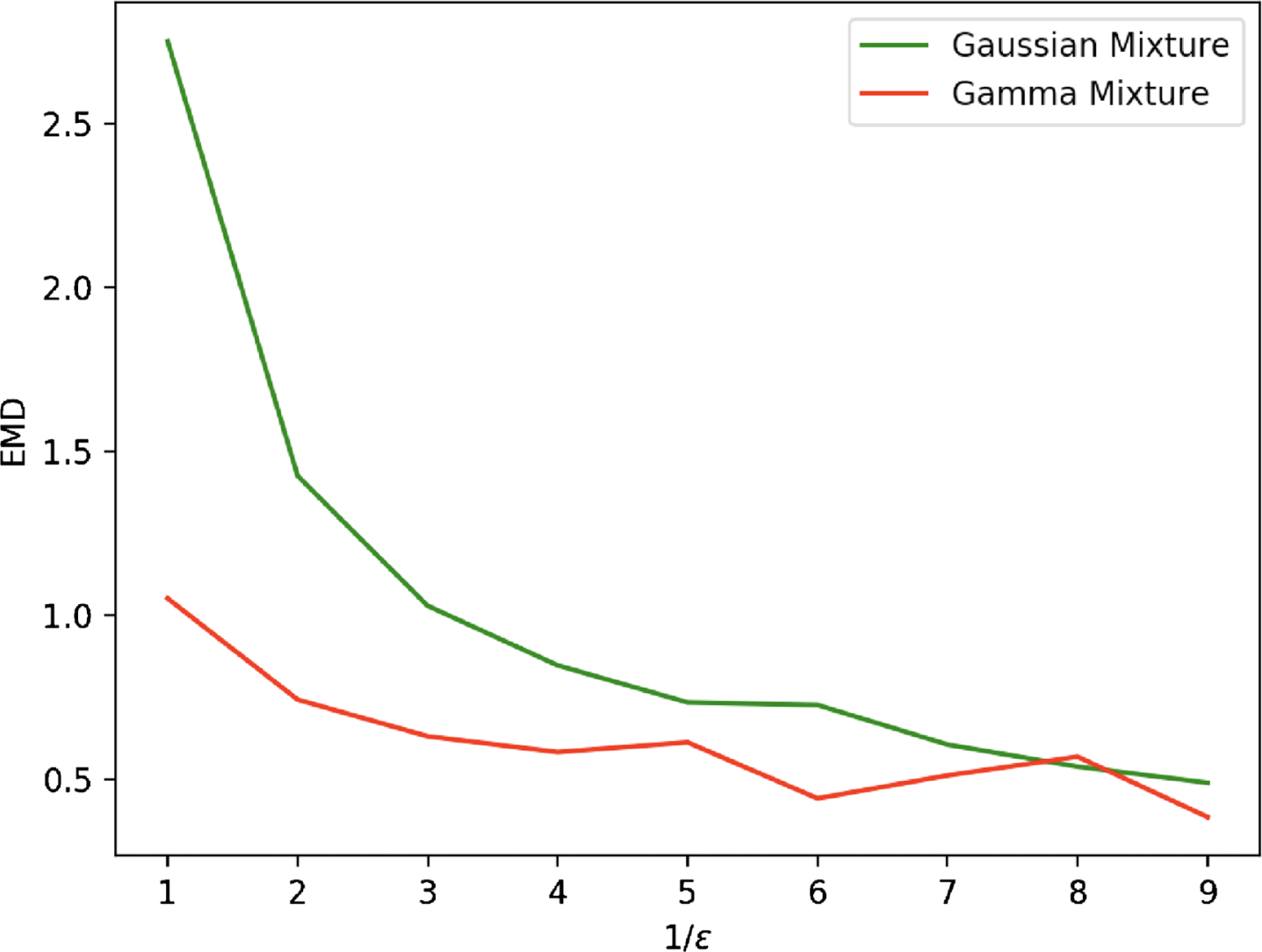
Fig. 3

Evolution in function of 1/ɛ of the Wasserstein distances between the empirical distribution associated to a set of 2000 cells, simulated with the model (3), and both the Gamma mixture approximation (6) (in red) and a GMM approximation (in green), for the toggle-switch network described in Table 1.

3.2Linking a GRN to mixture parameters

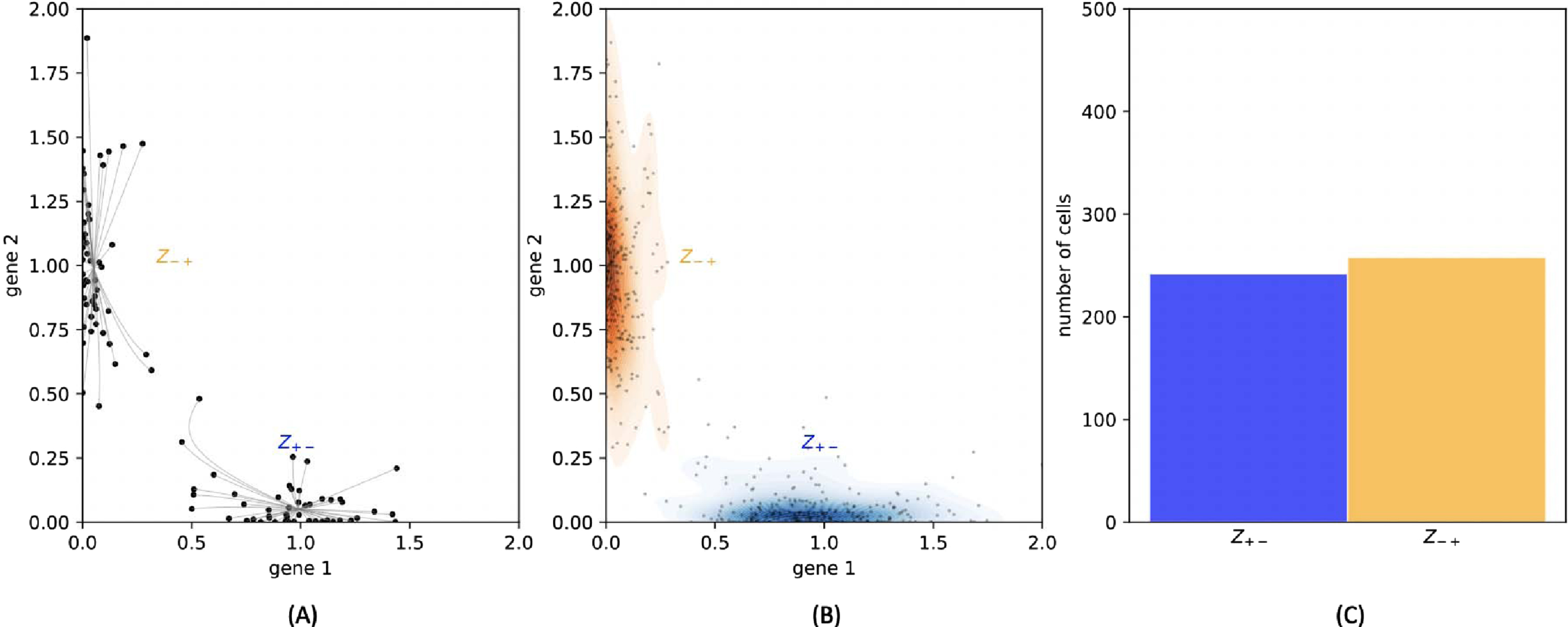
Building an analytical link between the GRN and the mixture parameters is generally out of range. Indeed, even if it was possible to solve explicitly the equation (5) defining the equilibrias associated to a GRN, it would remain challenging to study their stability in order to identify the attractors. Moreover, the probability vector μ is obviously linked to the transition rates of the coarse-grained model, which we recall to be very difficult to estimate from a GRN [51]. However, these parameters can be obtained with a simple numerical method, which consists in sampling a collection of random paths in the gene expression space: the distribution of their final position after a long time approximates the stationary distribution on proteins. We can then use these final positions as starting points for simulating the deterministic trajectories, given by the system (4), with an ODE solver: each of them converges to one of the stable equilibrium points. This method allows to obtain all the stable equilibria corresponding to sufficiently deep potential wells (see Figure 4(A)). Possible other potential wells can be omitted because they should correspond to basins that the process has very low probability of visiting, which do not impact significantly the coarse-grained Markov model. Repeating this operation for thousands of cells, we can find a vector μ describing the ratio of cells belonging to each basin (see Figures 4(B) and 4(C)). When the number and length of the simulations are large enough, the vector μ should be a good approximation of the stationary measure on the basins.

Fig. 4

(A): 100 cells are plotted under the stationary distribution. The relaxation trajectories allow to link every cell to its associated attractor. (B): 500 cells are plotted under the stationary distribution. They are then classified depending on their attractor, and this figure sketches the kernel density estimation of proteins within each basin. (C): The ratio of cells that are found within each basin gives an estimation of the stationary distribution on the basins.

3.3Mixture approximation of time-varying distribution

In the mixture approximation, the marginal on proteins of the stationary distribution of a single cell is characterized by a hidden Markov model: in each basin z ∈ Z, which corresponds to the hidden variable, the vector P is randomly chosen under the quasistationary distribution uˆz of X ∣ Z = z. Therefore, the mixture distribution can also be used as a proxy for the time-varying distributions of the bursty model (3). Denoting μ_t the distribution on the basins at any time t, and considering that a cell reaches almost immediately its quasistationary distribution after entering in a basin, we obtain the approximation:

We remark that with the method described in Figure 4, it would be possible to miss some basins that are important for describing the network, but which would not appear in the stationary distribution. It is expected to be a common situation for networks showing complex behaviours, as feedback loops or unbalanced branching structure, because the probability after a long time may be too weak for some basins to be visited, while playing an important role in the process beforehand. For such networks, the method should then be applied on a series of timepoints, and the union of all the basins identified at every timepoint should be considered (fixing the value μ_t (z) =0 for basins z that are not observed at time t). In that point of view, the basins appearing in the stationary distribution can be considered as (almost) absorbing states of the coarse-grained model.

Altogether the reduction and methods described above establish a formal basis for the definition of a simplified epigenetic landscape given a GRN, under the form of a mixture model. As the mixture parameters seem possible to obtain from a single-cell dataset (see Section 5.2), it would be fruitful to use the same formalism to assess the inverse problem of inferring the most likely GRN, given an (experimentally-determined) cell distribution in the gene expression space, a notoriously difficult task [16, 39].

4.1Linking the GRN and the attractors

The main idea of the method consists in using the fact that all the attractors P_z of the bursty model verify the equation (5), i.e that for all i = 1, ⋯ , n, : kon,iθ(Pz)=cid1,iPz,i .

Thus, from the definition of kz,i=kon,iθ(Pz) , we have the relation:

4.2GRN inference from a Gamma mixture as a minimization problem

GRN inference from a Gamma mixture is formally equivalent to identifying an adapted function R such that the "real" GRN θ^* associated to a set of mixture parameters α would be defined by

Regarding to the analysis which has been made in Section 4.1, a natural candidate for this function is

5.1Simplified statistical model for the data

Along with the system of n coupled systems of the form (3) describing proteins dynamics, as presented in Section 2.2, we obtain when ɛ ⪡ 1, i.e when the bursts are frequent in regard to proteins dynamics, a quasi steady-state approximation for the conditional distribution of M given P. Under this approximation, mRNAs levels M_i are independent conditionally to the protein vector, and follow Gamma distributions depending on P:

Contrary to what has been done in [15], where the inference strategy consists in treating proteins level as latent variables and using the law on mRNAs knowing proteins as a statistical likelihood for the data, we are going to use the analysis provided in Section 3 to directly estimate the set of mixture parameters α from the data without the need of proteins quantity. The main idea is the following. On one side, the only information on the proteins that can be obtained is contained in the value of k_on,i (P). On the other side, proteins being known to be less noisy than mRNAs, a vector P characterizing a cell in the gene expression space is going to be generally close to one of the attractor. Moreover, the functions k_on,i (P) are almost constant within each basin, and in particular around their attractor. Thus, the precise knowledge of the proteins quantity can be considered out of reach from scRNA-seq data, and the best information on proteins we can get from the marginal distribution on mRNAs of a gene i is the set of the modes of bursts frequency normalized by the degradation rate, that is kz,id0,i .

We finally derive a simplified statistical model, making appear the distribution of mRNA counts as a mixture of negative binomial:

5.2Inference procedure

We now describe the inference procedure for a set of l timestamped scRNA-seq data M = (M_t1, ⋯ , M_tl), where each M_tk is a matrix of gene expression containing the n_tk cells (x1k,⋯,xntkk) . We decompose the algorithm in 2 steps:

5.2.2Regression

First, in order to reduce the number of parameters and since protein levels P_i are not observed, we can arbitrarily set:

(11)

s1,i=d1,id0,ikoff,ik1,is0,i,

which leads to ci=k1,id1,i . Injecting this value in the formula (5), the attractors are then defined for any z ∈ Z by the formula: Pz=kzk1 . It is worth noticing that the choice of this scaling may not affect the accuracy of the inference. Indeed, the value of the parameter s_1,i only affects the number of proteins P_i that are created when M_i is positive: the value of P_i is then proportional to s_1,i. As every parameter θ_ij affects the dynamics of the process through the value of the product θ_ij × P_i in the function k_on,j, considering such scaling for s_1,i will only affect the scaling for the interaction coefficients θ_ij, but not the GRN topology.

The clustering step only allows to find the values of the vectors αz=kzd0 rather than k_z. This is not a problem since the fraction which characterizes P_z allows to simplify the term d₀, provided that k1d0 can be computed. We therefore consider that each gene reaches its minimal and maximal frequency through the timepoints, at least for some cells. Thus, we define for every gene i, k0,i=minzkz,i and k1,i=maxzkz,i , and equivalently:

(12)

α0,i=minzαz,i,α1,i=maxzαz,i.

We finally obtain a characterization of the attractors which is directly accessible from scRNA-seq data:

(13)

Pz=αzα1.

Injecting (13) in the definition of R given by (9), we obtain the following characterization of a cost between a GRN θ and a vector α describing the approximate landscape of the model (1):

(14)

R(θ,α)=∑z∈Z∑i=1n(σiθ(αzα1)-αz,iα1,i)2.

In order to define a regression problem on the variable θ which may associate a vector α obtained in the clustering step (see Section 5.2.1) to a GRN, we add three modifications to the cost function R given in (14).

First, we solve the problem of the possibly too high number of basins due to the clustering method, that we mentioned in Section 5.2.1, by taking into account the weight of the basins in the cost function. Then, given that we have enough cells that are detected in existing basins, the "false" basins detected in the clustering step, which should not be associated to many cells, would almost not affect the inference.

Second, in line with the idea that missing interactions is preferable to inferring false interactions between genes, we decide to use a LASSO penalization, which is known to enforce the sparsity of the network. We also add a custom penalization to deal with oriented interactions. Indeed, for every pair of nodes {i, j} there are two possible interactions with respective parameters θ_ij and θ_ji, but it is likely that only one is actually present in the true network. Our method is likely to favor symmetric interactions because when an interaction is present in the network (e.g θ_ij > 0), then gene j is generally upregulated in the same time than gene i and it is hard to distinguish whether θ_ji > 0 or not. Then we want these two interaction parameters to compete each other, such that only one is nonzero after the regression step, unless there is enough evidence in the data that both interactions are present. We obtain the following penalization

(15)

|θ-θ0|=∑i,j=1n|θi,j-θi,j0|+12|θi,jθj,i|,

where θ⁰ is defined as the null matrix of size n if there is no prior information on the GRN. The coefficient in front of the product ∣θ_ji θ_ij∣ is chosen small enough to ensure that if both θ_ji and θ_ij have been detected at a timepoint, it would generally cost more to put one back close to 0 than to keep it at its computed value.

Third, the temporal dynamics of the process, when available, must be considered. As developed in Section 3.3, the basins that have to be taken into account are all the basins identified during the differentiation process, i.e in the different snapshots of the time-varying distribution. But three principal reasons lead to consider that we should not try to infer the network from all the basins at the same time:

• 1. We can generally see the effect of a GRN in a cell as a signal which is transmitted to the genes [5]. Before the signal has been completely transmitted in the network, many genes are likely to be in a state which does not reflect the GRN. At these moments, the cell is far from the equilibrium. For this reason we would like to take into account the first timepoints, where some genes have not seen the signal, in a weaker way than the last timepoints, where the signal has been well transmitted to all the genes.

• 2. A population of cells is likely to be more often observed far from the attractors before it has reached its equilibrium than after reaching it. This is due to the fact that when the distribution is far from the equilibrium, some shallow or even unstable basins can be explored, from which the cell can easily escape. In particular, the regions around bifurcations in the cell lineage are expected to be often identified as shallow basins. These basins should then almost be erased if deeper basins are explored afterwards. This also suggests that the first timepoints have to be taken into account in a weaker way than the final ones.

• 3. Finally, recalling that GRN inference is known to be generally a non-identifiable problem, we simply cannot neglect the information that is brought by temporal information when it is available.

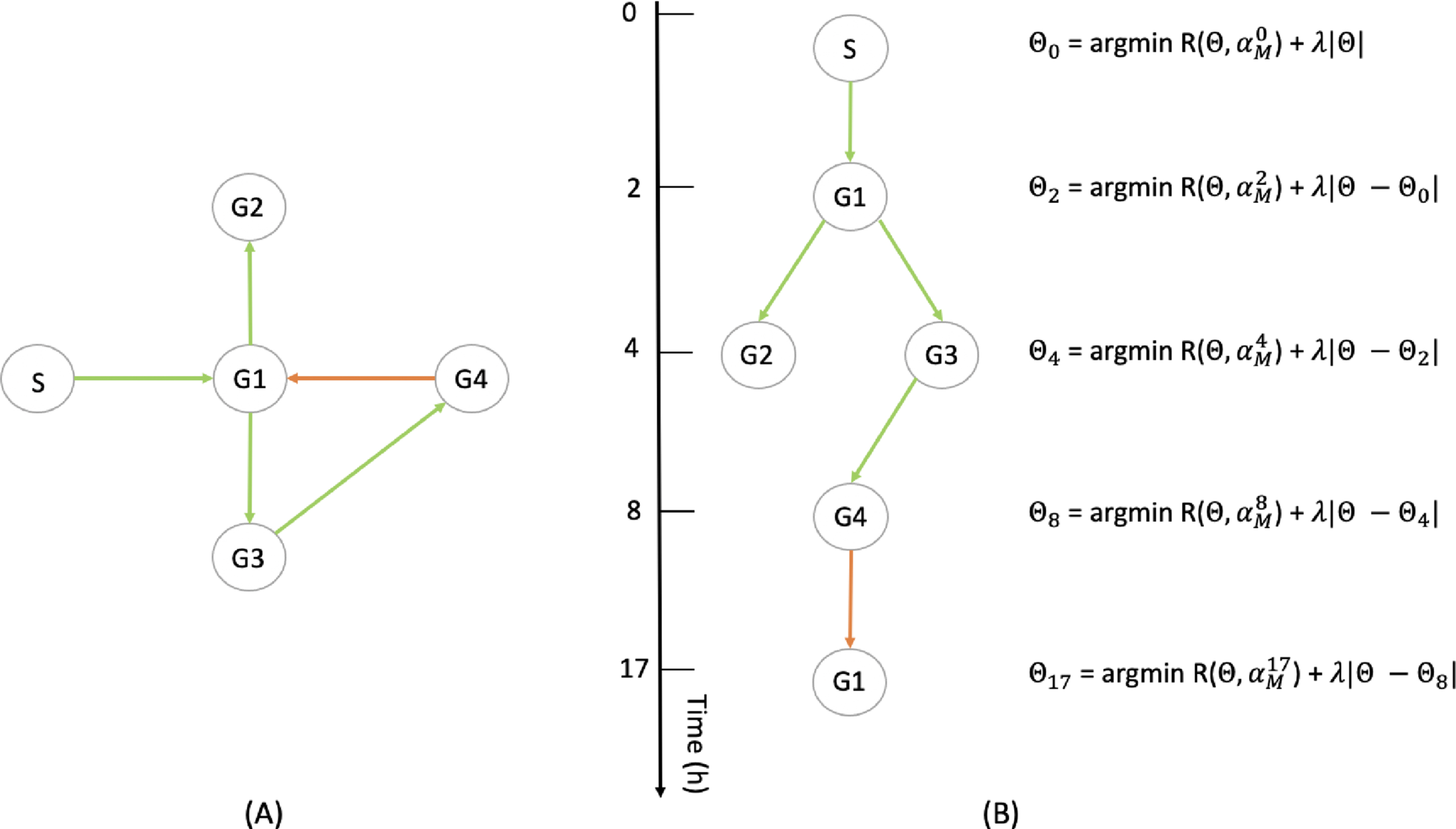
We thereby adopt an iterative approach: for each timepoint, the network is actualized by minimizing the function (14) with the penalization (15), taking as initial condition the network inferred at the previous timepoint. Then, we do not penalize the network itself but its variations to the initial condition. This should satisfy the points 1. and 2., because an erroneous interaction that would have been catched at an early timepoint would be conserved in the final network only if it does not appear in contradiction with the interactions that are inferred afterwards.

Finally, the regression step consists in solving successively, for k = 1, ⋯ , l, the problem

(16)

θk=argminθRk(θ,αMk)+λ|θ-θk-1|,

where θ⁰ is defined as the null matrix of size n, |θ - θ^k-1| is given by (15), λ is a penalization coefficient and the function R is defined for every θ and αMk={(μtk(z))z∈Z,(αz)z∈Z} by:

(17)

Rk(θ,αMk)=∑i=1n∑z∈Zμtk(z)(σiθ(αzα1)-αz,iα1,i)2.

The procedure is illustrated in Figure 5. For the applications presented in Section 6, the value of the coefficient λ has been calibrated in order to be optimal for various datasets simulated from randomly-generated tree-like networks, like those studied in Section 6.6.

Fig. 5

(A) Example of a 4-genes network (G1 to G4) with a stimulus (S) (see Section 6.1). (B) Illustration of the method described in Section 5.2.2: the interactions being observable only at some particular timepoints, they are progressively inferred, each optimization taking into accounts the interactions that are observed on the previous ones.

Interestingly, the cost function (17) can be obtained as the particular case of a more general method for linking a GRN to a set of mixture parameters in the case where single-cell proteomic data were available, and that mRNAs are seen as a proxy for the proteins level. We present this method in Appendix C.

We underline the fact that the function σ ^θ, defined in (2), depends only on the GRN θ and αzα1 , which can be directly estimated from scRNA-seq data, using the method described in Section 5.2.1 and the relations (12). Thus, we do not need to make any assumption on the value of the hyperparameters of the model, not even the ratio d0d1 as it was the case in [15]. This is due to the fact that we do not infer the protein distribution but only the values of its main modes, which are completely characterized by the mean of the proteins distribution within each basin, and do not depend on its variance.

The two-steps method presented in Sections 5.2.1 and 5.2.2, that we call CARDAMOM (Cell types Analysis from scRna-seq Data Achieved from a Mixture MOdel), shows good results for the simulated datasets that are presented in Section 6.

6.1Simulating data with stimulus

The simulations of the model (1) are performed with the python package HARISSA presented in [15], which is based on an efficient thinning method for simulating the model (1). For reproducing in vitro differentiation processes, we first simulate every network until reaching a first equilibrium before t = 0. At t = 0, we introduce a new gene called "stimulus", the proteins level of which is artificially maintained at the value of 1. This value corresponds to to its highest possible attractor: indeed, the proteins scaling (11) implies that no coordinates of the attractors can be greater than 1 in the gene expression space. Proteins being much less noisy than mRNA (i.e d0,id1,i⪢1 ), the protein level associated to a gene is expected to be close to the attractor associated to the basin it belongs to, and forcing a gene to be fully expressed in the model (1) with the scaling (11) is equivalent to force its value to 1. Then, the stimulus represents the effect of an artificial perturbation in the differentiation environment inducing cells to evolve towards a new equilibrium. The datasets correspond to the sample of independent cells at a sequence of timepoints.

6.2Inference of a toggle-switch network from a static expression data sampled under the long time distribution

We first evaluated the ability of CARDAMOM to find the parameters of a 4-genes network consisting in 2 independent toggle-switch of the same form than the one described in Table 1. To this aim, we simulate 10 dataset by sampling 50 independent cells at 2 timepoints 0 and 20h. In that case, the stimulus has no effect on the system. Inference is then independently performed for every datasets and the mean of all the significant values obtained for each network is presented in Figure 6, compared to the network used for the simulations. We observe in Figure 6 that the algorithm allows to reconstruct very well the topology of the network, detecting which pairs of genes are in relation together and the sign of the interactions. All other coefficients of the GRN matrix are smaller than 0.3, which can be considered as a residual noise with regards to the principal edges. However, the algorithm computes the values of the coefficients up to a multiplicative factor, which is in line with the limitations we pointed out in Section 5.2.3.

Fig. 6

Inference of a 4-genes network (G1 to G4) consisting in two independent symmetric toggle-switch networks with parameters described in Table 1. The stimulus (S) has no effect on the network, but is nevertheless represented in order to verify whether the inferred network takes it into account or not. The network used for simulating the datasets in (A) is compared with the network inferred by CARDAMOM in (B).

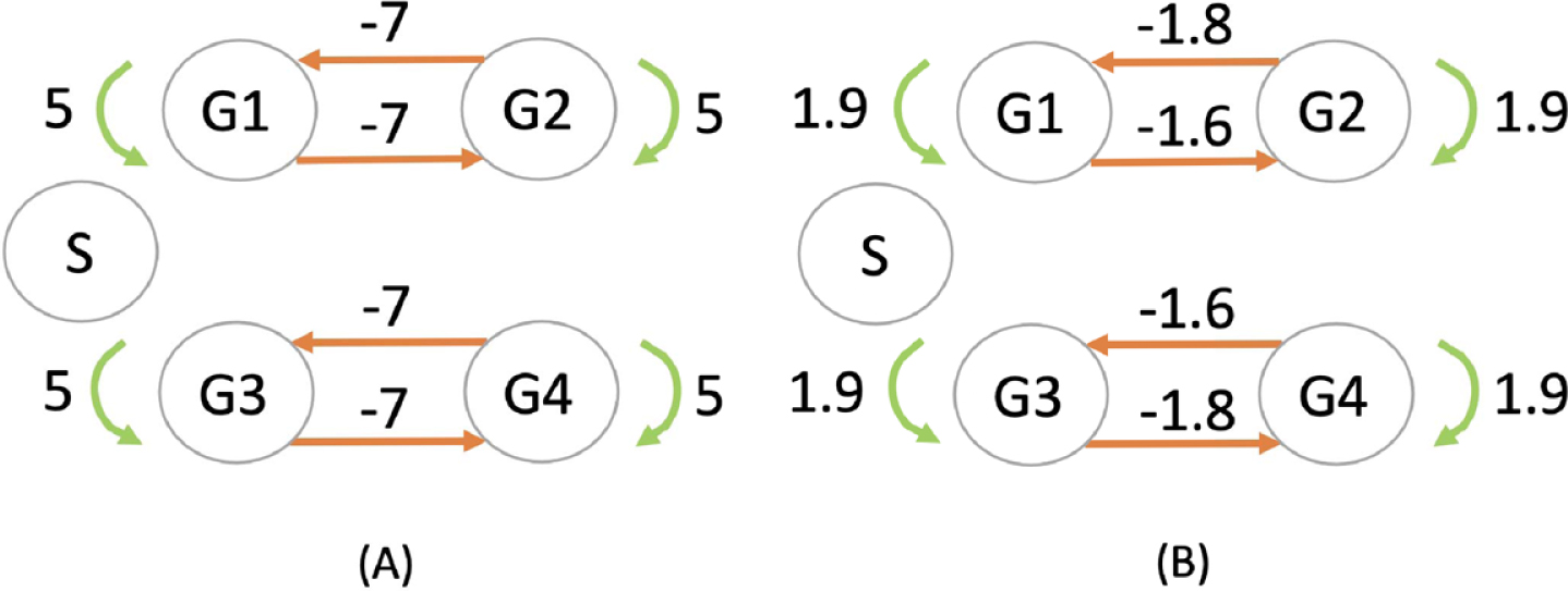
We remark that the algorithm slightly overestimates the diagonal coefficients, which correspond to self-regulation parameters of the genes: the problem of the inference of these parameters being notoriously difficult to infer reliably [40], we will not take into account the diagonal coefficient of the GRN matrix for evaluating the algorithm performances in the following.

6.3Inference of a 4-genes network with branching and feedback loop from timestamped data

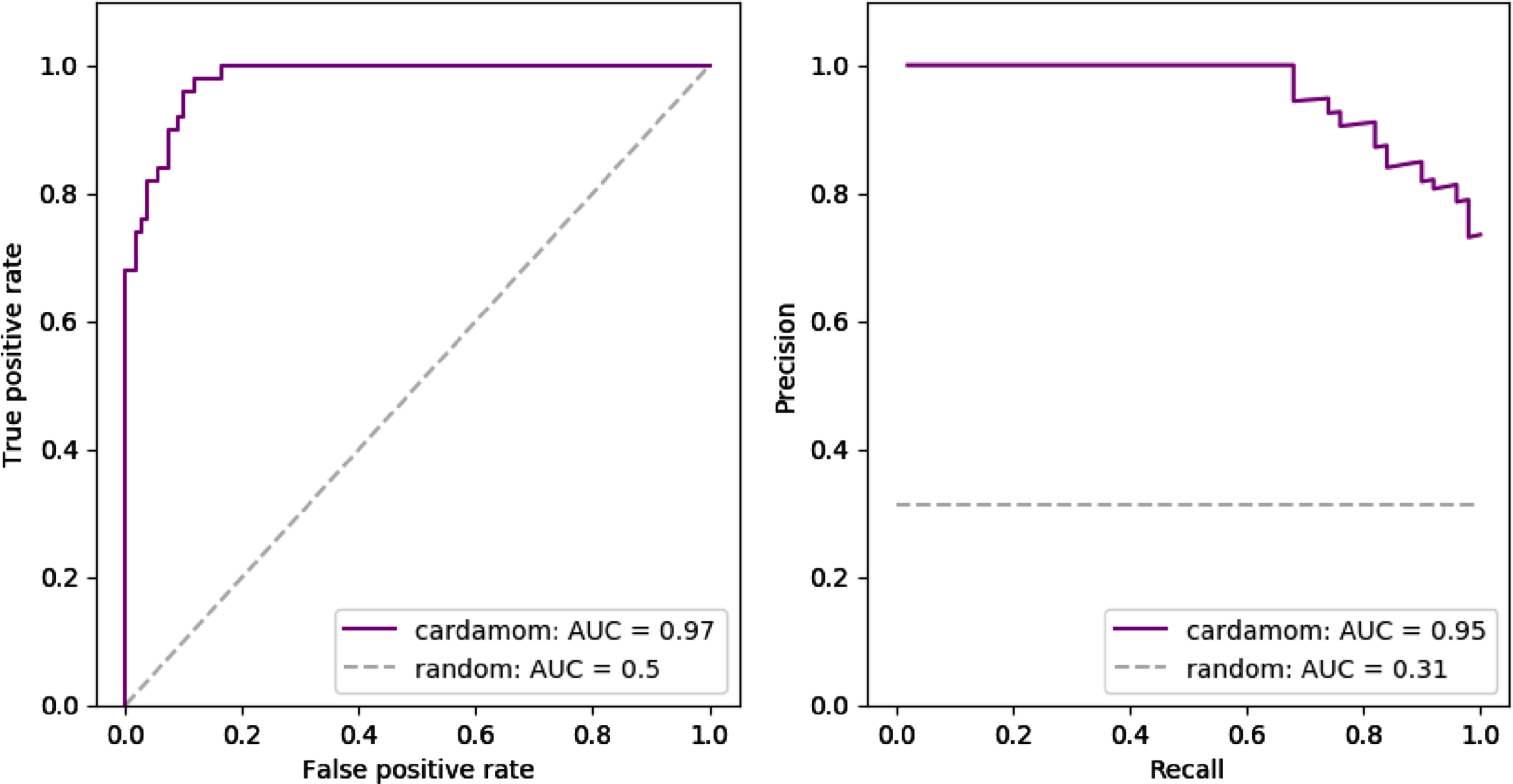
We now evaluate CARDAMOM on the 4-gene network described in Figure 5 and Table 2. Although such a small network may appear very simple, it already has some interesting features (branching, feedback loop with inhibition) and is interesting for inference. To this aim, we simulate 10 datasets by sampling independent cells at 10 time points t = 0, 2, 4, 6, 8, 11, 13, 15, 17, and 20h, with 50 cells per timepoint (then 500 cells in total for each dataset). Inference is independently performed for every dataset and the results are merged into receiver operating characteristic (ROC) and precision-recall (PR) curves that are shown in Figure 7. CARDAMOM turns out to reconstruct very efficiently the topology of the network. We precise that the sign of the interactions that are inferred is well preserved comparing to the original network.

Fig. 7

Inference results for the 4-gene network described in Table 2. Performances are measured in terms of receiver operating characteristic curves (ROC) and precision-recall curves (PR) obtained for 10 independently simulated datasets. Each dataset contained the same 10 timepoints and 50 cells per time point. The dashed gray line indicates the average score that would be obtained by the random estimator (detecting a link or not with equal probability).

6.4Reproduction of the data

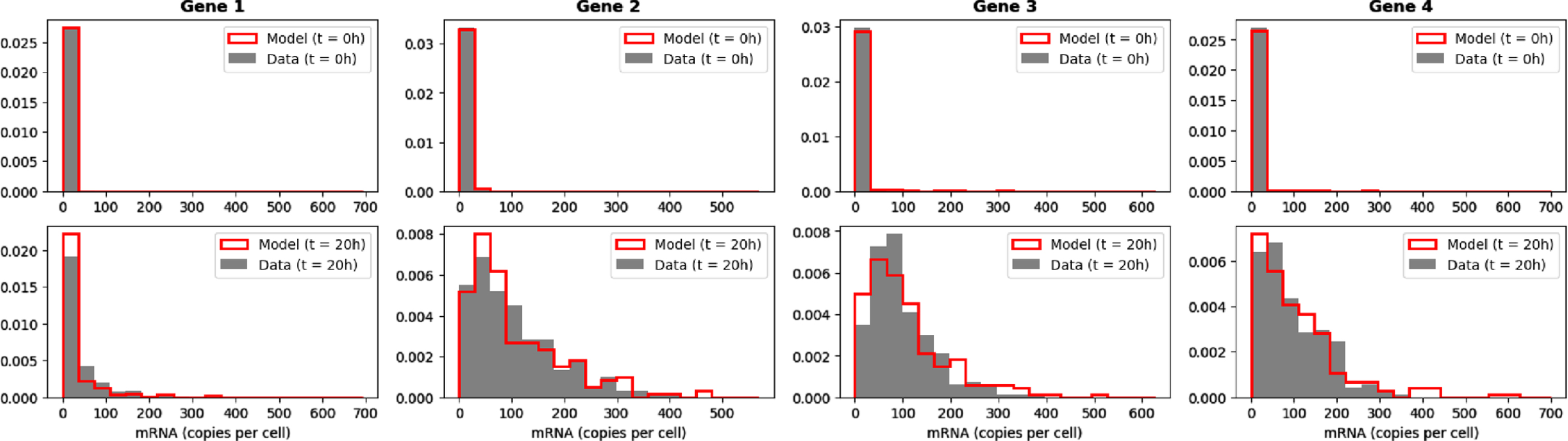
The bursty model (1) with k_on functions defined by (2) can satisfactorily produce expression data for which marginal distributions of genes are close to mixtures of negative binomial distributions, which is known to be biologically relevant. In line with what was discussed in Section 5.2.3, we do not expect the temporal dynamics associated to the network inferred by CARDAMOM to be synchronised with the original data. We then focus on the comparison between the initial and final distributions of the model when simulated by the network presented in Table 2 and the network inferred in Section 6.3, observed at respectively 0h and 20h after applying the stimulus (see Figure 9). We underline the fact that we do not take the initial distribution of the data to initialize the simulation, but we rather sample a distribution using the inferred network with the stimulus fixed to 0.

Fig. 9

Comparison of the initial (t = 0h) and final (t = 20h) empirical marginal distributions of 4 genes simulated by the mechanistic model with the GRN described in Table 2, and the dataset simulated from the GRN inferred by CARDAMOM from the previous dataset (with 200 cells per timepoints).

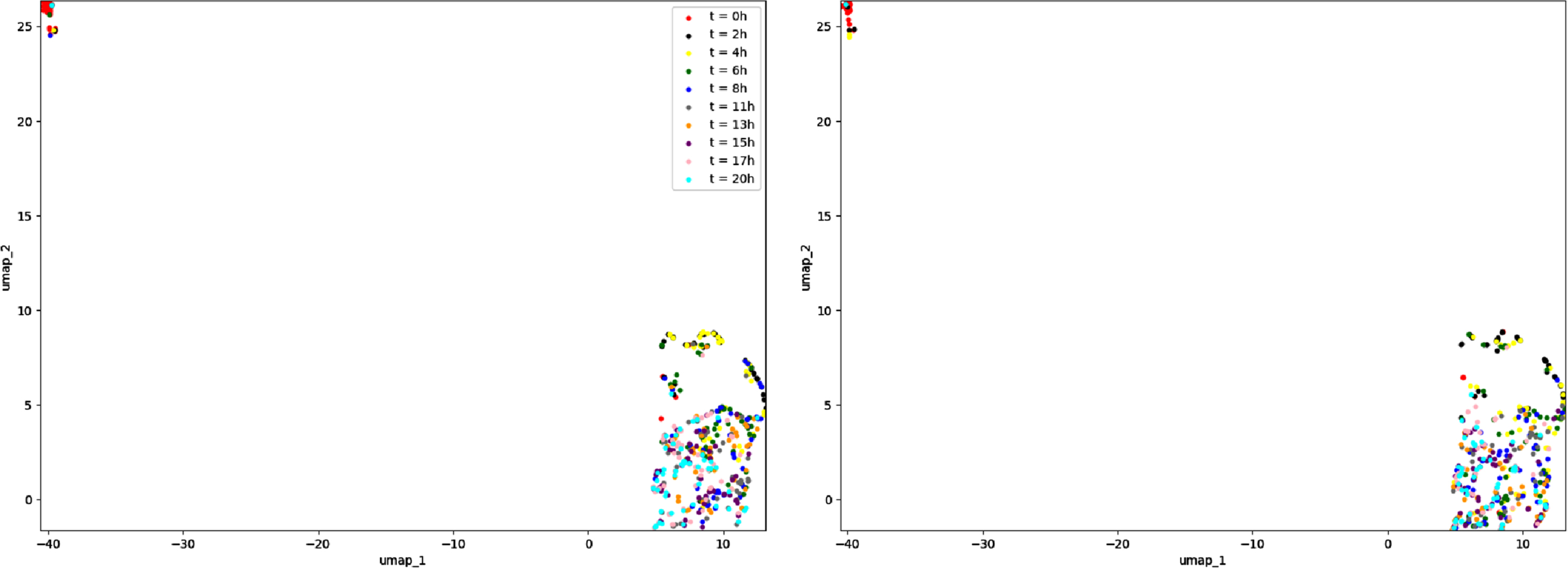
We also compare in Figure 10 the two temporal dynamics of the two complete datasets, one used for the inference and one simulated with the inferred network. The data are projected altogether with the method umap and we show on each subfigure the cells corresponding to one of the datasets. These cells are then classified depending on the time where the measures are realized after applying the stimulus. The results suggest that the model has been relatively well calibrated through the inference procedure.

Fig. 10

Representation in 2 dimensions of (A) the dataset used for the inference, simulated from the GRN described in Table 2 and (B) the dataset simulated from the GRN inferred by CARDAMOM. Each dataset contains 500 cells divided in 10 timepoints.

6.5Simplification of the method for sigmoidal burst rate functions

The clustering method described in Section 5.2.1 allows to take into account any number of modes for the burst frequency associated to each gene. However, it is natural to ask if such complexity is compatible with the one allowed by the choice of the functions k_on,i. In fact, when these functions have the sigmoidal form described in (2), they cannot be expected to be associated to a high number of attractors with intermediate values comprised between k_0,i and k_1,i. A rough simplification consists in considering that every gene is the result of a mixture of the form (6) with only two modes, which can be expected to be close to the values of k_0,i and k_1,i. Following this idea, the clustering step of CARDAMOM can be replaced by a simple binarization of the cells, where the mRNA value measured for each gene is classified as belonging either to the mode k_0,i or k_1,i, with a likelihood ratio between the two negative binomials associated to these parameters. We underline that this approximation does not mean that the data always exhibits strong bimodality. It only means that the fact that they are sometimes observed far from their extremum, which is expected at least during the period of transition after applying the stimulus, does not mean that these transitory states are stable.

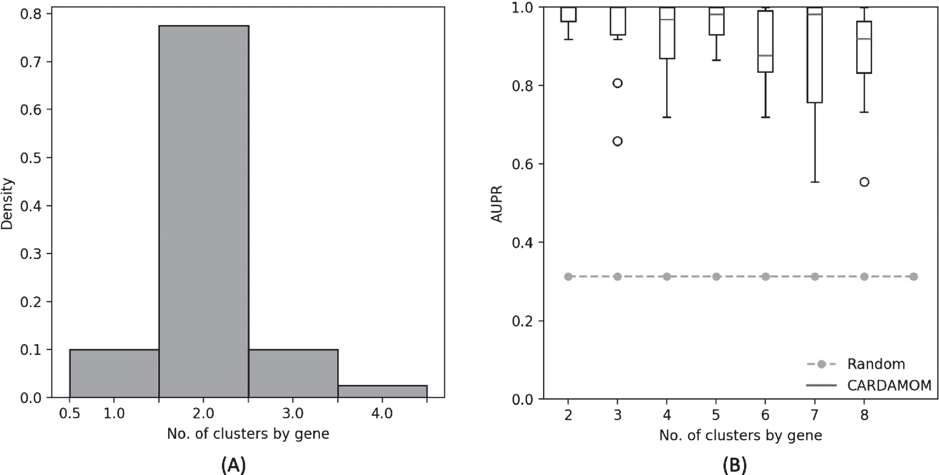
The simplification consisting in imposing a number of clusters equal to 2 for each gene would not affect the efficiency of the algorithm for the 4-genes network studied in Section 6.3. Indeed, we observe in Figure 8(A) that the RJMCMC algorithm applied to each gene of the network for every datasets simulated from this network usually computes a number of clusters equal to 2, and in Figure 8(B) that imposing a number of cluster greater than 2 makes slightly decreases the efficiency of the algorithm. We discuss in Section 7.4 the consequences of the accuracy of such simplified method, which may argue in favor of more complex burst functions than the ones of the form (2), or even adaptive functions depending on the clustering step described in Section 5.2.1.

Fig. 8

(A): Distribution of the number of clusters found by the RJMCMC algorithm during the clustering step for each gene of the 4-genes network described in Table 2. (B): Comparison of the performances of CARDAMOM for the same network, when imposing different values for the number of clusters in the clustering step. Performances are measured in terms of area under precision-recall curve (AUPR), based on 10 datasets corresponding to the same network.

6.6Application to larger networks

We now consider the cases of tree-like activation networks of 5, 10, 20, 50 and 100 genes. For each case, we simulate ten datasets corresponding to 10 random networks of the same size, that sampled from the uniform distribution over trees rooted in the stimulus [15]. All datasets contain the same 10 timepoints t = 0, 2, 5, 8, 11, 13, 16, 19, 22, and 25h, with 100 cells per timepoint (then 1000 cells in total for each dataset). Inference is then independently performed for all dataset with CARDAMOM and the state-of-the-art method GENIE3 [19]. The results are presented in terms of Area Under Precision-Recall curves (AUPR), in Figure 11A). CARDAMOM turns out to reconstruct more efficiently the topology of the network than GENIE3. The strong decrease in performance when the number of genes gets higher is due not only to the lack of data per timepoints in regards to the number of interactions, but also to the choice of the timepoints. Indeed, a sequence of timepoints that is too coarse to catch the dynamics would lead to a lack of accuracy in the inference, and a sequence which is too tight would often be too short, leading to miss the activity of some genes. This appears to be the case from 20 genes in Figure 11A).

Fig. 11

(A) Evolution of the performances of CARDAMOM and GENIE3 when increasing the number of genes. For each number of genes, we represent a boxplot of the AUPR scores computed for ten datasets simulated with 10 different randomly generated tree-like networks. (B) Evolution of the average computational time measured for inferring the tree-like networks with respect to the number of genes.

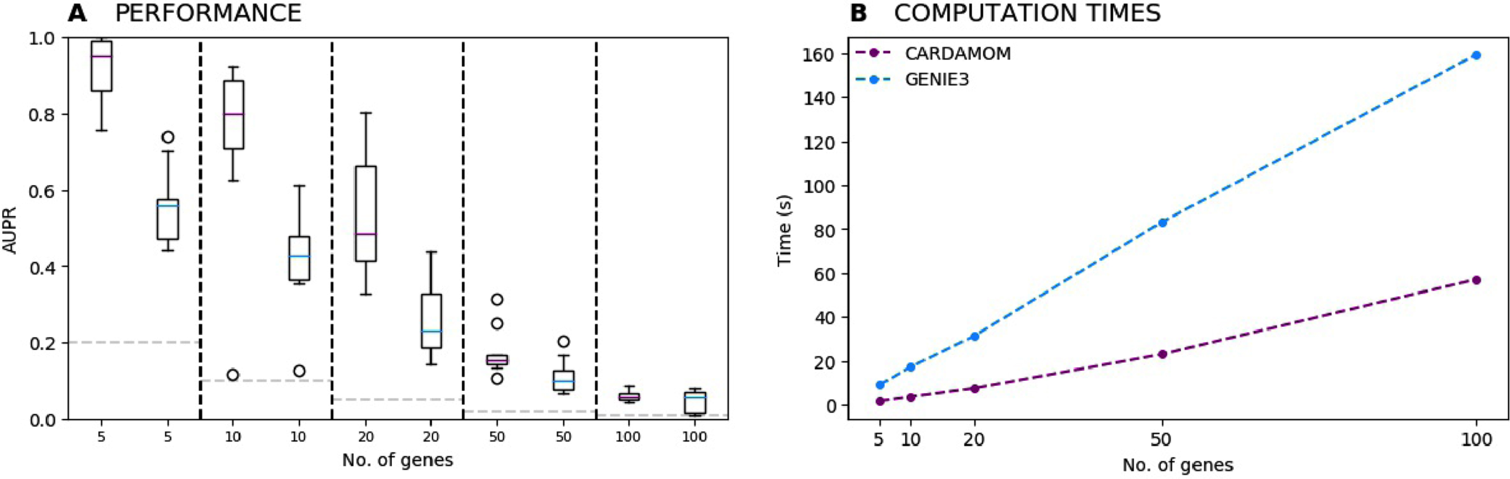
For every size of network, an average runtime is obtained after inferring the 10 datasets associated to the 10 tree-like networks, on a 16-GB RAM, 2,4 GHz Intel Core i5 computer. We see in Figure 11B) that for both algorithms the computational speed increases linearly with respect to the number of genes, with a slope which is significantly lower for CARDAMOM. These results show that the algorithm is suitable for realistic number of genes and cells.

7.1Importance of the clustering

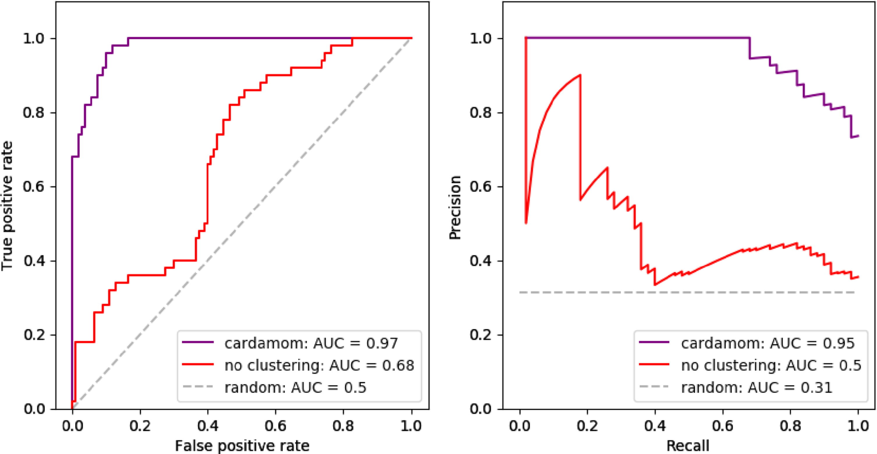
The attentive reader should have remarked that the function (17) which is optimized in the second step of CARDAMOM appears very simple and close to a generalized linear model, which is surprising for an analysis based on a mechanistic model. It is then natural to ask whether the clustering step remains important or if it is possible to reduce the method to the regression step by identifying each cell to a distinct attractor without losing an important accuracy (the clustering step would then simply consists in rescaling each count of a gene i by the parameters c_i). We compare in Figure 12 this coarse simplification with CARDAMOM on the datasets used in Section 6.3. We observe that such simplification generates a significant decrease in accuracy, confirming that the method cannot be reduced to such generalized regression.

Fig. 12

Analogy of Figure 7, where we compare (A) the ROC curves and (B) the PR curves of the GRN reconstruction performed by CARDAMOM with clustering (in purple) and without clustering (in red, considering that there are as many clusters as cells in each dataset).

7.2Limits of the method for finding the developmental landscape

In this section, we come back on the Gamma mixture approximation (6) and its limitations for describing the developmental landscape of differentiation, in order to remove some of the confusion that might arise from misuse of this approximation. As we presented in Section 3, this mixture approximation is based on two assumptions:

This limitation is very hard to overcome. For this sake, we should either get knowledge on the values of the cells distribution on saddle points of the landscape which are located in areas of the gene expression space where it is very unlikely to find cells, which would require to have thousands of cells just for a small network, or to take into account explicitly the value of time in the inference method. The latter point would require to have analytical results on the temporal distribution of cells in the gene expression space, which is generally out of range for realistic models like (1). For example, using the temporal dynamics of the probability vector μ_t on the basins for reconstructing the transition rates (see Section 3.3) would be challenging as an analytical link between these transition rates and the GRN can only be obtained up to a prefactor, which does not depend on the scaling factor ɛ but is specific to each transition [51]. The only solution seems then to combine analytical results with simulations, in the same philosophy than [5], but this leads to much more complex and time-consuming algorithms that the one which is developed in this article. To our point of view, this also argues against methods where a mixture model is used for reconstructing the temporal dynamics of a metastable process from stationary distributions [37].

7.3Applicability of CARDAMOM to real single-cell datasets

The algorithm CARDAMOM has been shown to reconstruct accurately a most-likely GRN from timestamped in silico datasets, through the estimation of the metastable parameters associated to these data. It is then natural to ask whether the method could deal with real datasets or not. The method for estimating the metastable parameters should be well suitable for real datasets, provided that the Negative Binomial mixture approximation of mRNAs is accurate, and we have seen in Section 6.6 that the algorithm is suitable for realistic number of genes and cells. The main difficulty that could appear would then be related to the decrease in the performance of the algorithm with the number of modes appearing in the sample. Indeed, we recall that the regression step aims to infer a GRN matrix of size n × n from the values of the functions k_on,i at each attractor. First, it implies that too few clusters in the sample would mean too little information for the inference. Second, as developed in Section 6.5, too many clusters for each gene would make the sigmoidal bursts rate functions unsuitable, which could also lower the performances of the algorithm. Then, the level of multistability seems then to be critical for the accuracy of the inference. For the first point, we argue that regarding the noisy nature of mRNA counts, it is impossible to infer a reliable GRN when there is not enough multistability in the sample, i.e when the marginal distribution of mRNA associated to each gene is described by a simple negative binomial, the parameters of which does not evolve in time. We discuss in Section 7.4 the implications of the second point in terms of modeling.

To go further, we recall that the mathematical analysis beyond CARDAMOM lays on the point of view that cell differentiation processes can be coarsely reduced into a discrete process on a limited number of cell types, i.e that the main ingredients for characterizing stochasticity are the frequency modes describing the cell types and the random transitions between them, which is commonly accepted since [18]. Such transitions have been for example recently proposed as the basis for facilitating the concomitant maintenance of transcriptional plasticity and stem cell robustness [55]: in this case, the authors had proposed a phenomenological view of the transition dynamics between states, and our work may typically connect this cellular plasticity to an underlying GRN dynamics. This connection between a GRN and associated cell states should also be used for the quantitative modeling of stochastic state transitions underlying the generation of diversity in cancer cells [14, 56], or for investigating transitions between the large diversity of clusters that can be observed in human ES cell differentiation datasets [29].

7.4Gene expression as a neural network

Interestingly, CARDAMOM appears close to a machine learning approach. Indeed, since each function k_on,i is independent from the others, depending only on the i^th line of the matrix θ, the regression step is fairly close to parallel regressions of each gene on the others. The choice of sigmoidal bursts rate functions makes these regressions appear as the learning step of an artificial neural network, which is simply a set of one-layer perceptron for each gene coupled by the crossed-penalization between the symmetric coefficients of the matrix θ (see (15)). In the light of this framework, the first step of the algorithm can be seen as an identification of the outputs from the data, by identifying the mode associated to each mRNA count. For sigmoidal bursts rate functions, we have seen in Section 6.5 that it is reasonable to consider only two modes. This makes the clustering step close to the prepossessing of a Boolean network analysis, which consists in assigning every cell to the state of a Boolean model, where a 0 may rather take any values between 0 and 1. Without crossed-penalization, the second step would exactly consist in learning the parameters of a perceptron as represented in Figure 13, where each line of the matrix θ corresponds to the weight of the perceptron. The method then builds an interesting link between machine learning and dynamical modeling.

The results presented in Section 6.5 let us suppose that the sigmoidal bursts rate functions of the form (2) on have a limited complexity, i.e that they are not able to catch a multistability which would be associated to more than two potential wells for each gene. Thus, when applying the clustering step to a dataset showing an important multimodality, at least for some genes, the sigmoidal function may be not adapted for modeling the behaviour of the underlying process.The clustering step of CARDAMOM, described in Section 5.2.1 could therefore be seen as a preliminary to the choice of the "right" bursts rate function that should be used for minimizing the risk (17) (see Section 5.2.2): this function should be chosen in accordance with the number of modes detected for each gene. The neural network framework introduced above is interesting, as it suggests that the choice of the bursts rate function could correspond to the choice of the number of layers in the neural network of Figure 13. In that point of view, the work achieved in this paper treats the basic case of one layer, which could be extended, although the interpretability of the nodes for more than one layer remains an open question. We believe that this adaptability is necessary when dealing with highly complex single-cell data.

Fig. 13

CARDAMOM can be interpreted as the learning of a perceptron, where the clustering step (Section 5.2.1) corresponds to the classification of the data, regarding to their associated modes of frequency, and the regression step (Section 5.2.2) to the identification of the weights of the perceptron, corresponding to the GRN.

References

[1] | Akers K. and Murali T.M. , Gene regulatory network inference in single cell biology, In: Current Opinion in Systems Biology (2021). |
[2] | Albayrak C. , et al., Digital quantification of proteins and mRNA insingle mammalian cells. In: Molecular Cell 61: (6) ((2016) ), pp. 914–924. |
[3] | Antolovic V. , et al., Generation of Single-Cell TranscriptVariability by Repression. In: Curr Biol 27: (12) ((2017) ), 1811–1817 e3. |
[4] | Bizzarri M. , et al., Gravity Constraints Drive Biological Systems Toward Specific Organization Patterns: Commitment of cell specification is constrained by physical cues. In: Bioessays (2017). |
[5] | Bonnaffoux A. , et al., WASABI: a dynamic iterative framework forgene regulatory network inference. In: BMC Bioinformatics 20: (1) ((2019) ), pp. 1–19. |
[6] | Bouguila N. and Elguebaly T. , A fully bayesian model based onreversible jump MCMC and finite beta mixtures for clustering. In: Expert Systems with Applications 39: (5) ((2012) ), pp. 5946–5959. |
[7] | Braun E. , The unforeseen challenge: from genotype-to-phenotype incell populations. In: Rep Prog Phys 78: (3) ((2015) ), pp. 036602. |
[8] | Chan T.E. , Stumpf M. and Babtie A.C. , Gene regulatory networkinference from singlecell data using multivariate informationmeasures. In: Cell Systems 5: (3) ((2017) ), pp. 251–267. |
[9] | Coskun A.F. , Eser U. and Islam S. , Cellular identity at thesingle-cell level. In: Mol Biosyst 12: (10) ((2016) ), pp. 2965–2979. |
[10] | Dias J.G. and Wedel M. , An empirical comparison of EM, SEM and MCMCperformance for problematic Gaussian mixture likelihoods. In: Statistics and Computing 14: (4) ((2004) ), pp. 323–332. |
[11] | Faggionato A. , Gabrielli D. and Crivellari M. , Non-equilibriumthermodynamics of piecewise deterministic Markov processes. In: Journal of Statistical Physics 137: (2) ((2009) ), pp. 259. |
[12] | Gao N.P. , et al., Universality of cell differentiation trajectories revealed by a reconstruction of transcriptional uncertainty landscapes from single-cell transcriptomic data, In: bioRxiv (2020). |
[13] | Guillemin A. , et al., Drugs modulating stochastic gene expressionaffect the erythroid differentiation process. In: PLOS ONE 14: (11) ((2019) ), e0225166. |
[14] | Gupta P.B. , et al., Stochastic state transitions give rise tophenotypic equilibrium in populations of cancer cells. In: Cell 146: (4) ((2011) ), pp. 633–44. |
[15] | Herbach U. , Gene regulatory network inference from singlecell data using a self-consistent proteomic field. In: arxiv (2021). |
[16] | Herbach U. , et al., Inferring gene regulatory networks fromsingle-cell data: a mechanistic approach. In: BMC SystemsBiology 11: (1) ((2017) ), 105. issn: 1752-0509. |
[17] | Huang S. and Ingber D. , A non-genetic basis for cancer progressionand metastasis: selforganizing attractors in cell regulatorynetworks. In: Breast Disease 26: (1) ((2007) ), pp. 27–54. |
[18] | Huang S. , et al., Cell fates as high-dimensional attractor states ofa complex gene regulatory network. In: Physical Review Letters 94: (12) ((2005) ), pp. 128701. |
[19] | Irrthum A. , Wehenkel L. , Geurts P. , et al., Inferring regulatorynetworks from expression data using tree-based methods. In: PloS One 5: (9) ((2010) ), e12776. |
[20] | Kauffman S. , A proposal for using the ensemble approach tounderstand genetic regulatory networks. In: Journal of Theoretical Biology 230: (4) ((2004) ), pp. 581–590. |
[21] | Minoru Ko SH , A stochastic model for gene induction. In: Journal of Theoretical Biology 153: (2) ((1991) ), pp. 181–194. |
[22] | Li G.-W. and Xie X.S. , Central dogma at the single-molecule level inliving cells. In: Nature 475: (7356) ((2011) ), pp. 308–315. |
[23] | Lin Y.T. and Galla T. , Bursting noise in gene expression dynamics:linking microscopic and mesoscopic models. In: Journal of TheRoyal Society Interface 13: (114) ((2016) ), pp. 20150772. |
[24] | Mackey M. , Tyran-Kamińska M. and Yvinec R. , Moleculardistributions in gene regulatory dynamics. In: Journal of Theoretical Biology 274: (1) ((2011) ), pp. 84–96. |
[25] | Mar J. , The rise of the distributions: why non-normality is important for understanding the transcriptome and beyond, In: Biophys Rev (2019), pp. 89–94. |
[26] | Mar J. , The rise of the distributions: why non-normality isimportant for understanding the transcriptome and beyond. In: Biophysical Reviews 11: (1) ((2019) ), pp. 89–94. |
[27] | McInnes L. , Healy J. and Melville J. , Umap: Uniform manifold approximation and projection for dimension reduction, In: arXiv preprint arXiv:1802.03426 (2018). |
[28] | Mojtahedi M. , et al., Cell Fate Decision as High-DimensionalCritical State Transition. In: PLoS Biol 14: (12) ((2016) ), e2000640. |
[29] | Moon K. , et al., Visualizing structure and transitions inhigh-dimensional biological data. In: Nature Biotechnology 37: (12) ((2019) ), pp. 1482–1492. |
[30] | Moris N. and Arias A.M. , The Hidden Memory of Differentiating Cells. In: Cell Syst 5: (3) ((2017) ), pp. 163–164. |
[31] | Moris N. , Pina C. and Arias A.M. , Transition states and cell fatedecisions in epigenetic landscapes. In: Nat Rev Genet 17: (11) ((2016) ), pp. 693–703. |
[32] | Morris S.A. , The evolving concept of cell identity in the singlecell era. In: Development 146: (12) ((2019) ), pp. 1–5. |
[33] | Moussy A. , et al., Integrated time-lapse and single-celltranscription studies highlight the variable and dynamic nature ofhuman hematopoietic cell fate commitment. In: PloS Biol 15: (7) ((2017) ), e2001867. |
[34] | Nicolas D. , Phillips N.E. and Naef F. , What shapes eukaryotictranscriptional bursting? In: Mol Biosyst 13: (7) ((2017) ), pp. 1280–1290. |
[35] | Ochiai H. , et al., Stochastic promoter activation affects Nanogexpression variability in mouse embryonic stem cells. In: Scientific Reports 4: (1) ((2014) ), pp. 1–9. |
[36] | Papanicolaou G. , Asymptotic analysis of transport processes. In: Bulletin of the American Mathematical Society 81: (2) ((1975) ), pp. 330–392. |
[37] | Pearce P. , et al., Learning dynamical information from staticprotein and sequencing data. In: Nature Communications 10: (1) ((2019) ), pp. 1–8. |
[38] | Peccoud J. and Ycart B. , Markovian modeling of gene-productsynthesis. In: Theoretical Population Biology 48: (2) ((1995) ), pp. 222–234. |
[39] | Pratapa A. , et al., Benchmarking algorithms for gene regulatorynetwork inference from single-cell transcriptomic data. In: Nat Methods 17: (2) ((2020) ), pp. 147–154. |
[40] | Pratapa A. , et al., Benchmarking algorithms for gene regulatorynetwork inference from single-cell transcriptomic data. In: Nature Methods 17: (2) ((2020) ), pp. 147–154. |
[41] | Richard A. , et al., Single-Cell-Based Analysis Highlights a Surge in Cell-to-Cell Molecular Variability Preceding Irreversible Commitmentin a Differentiation Process. In: PloS Biol 14: (12) ((2016) ), e1002585. |
[42] | Richardson S. and Green P.J. , On Bayesian analysis of mixtures withan unknown number of components (with discussion). In: Journalof the Royal Statistical Society: series B (statisticalmethodology) 59: (4) ((1997) ), pp. 731–792. |
[43] | Rodriguez J. and Larson D.R. , Transcription in Living Cells:Molecular Mechanisms of Bursting. In: Annu Rev Biochem 89: ((2020) ), pp. 189–212. |
[44] | Sanguinetti G. , et al., Gene regulatory network inference: an introductory survey, In: Gene Regulatory Networks. Springer, (2019), pp. 1&23. |
[45] | Abhishek Sarkar K. and Stephens M. , Separating measurement and expression models clarifies confusion in single cell RNA-seq analysis, In: BioRxiv (2020). |
[46] | Semrau S. , et al., Dynamics of lineage commitment revealed bysingle-cell transcriptomics of differentiating embryonic stem cells. In: Nat Commun 8: (1) ((2017) ), pp. 1–16. |
[47] | Stumpf P.S. , et al., Stem Cell Differentiation as a Non-MarkovStochastic Process. In: Cell Systems 5: ((2017) ), pp. 268–282. |
[48] | Suter D.M. , et al., Mammalian genes are transcribed with widelydifferent bursting kinetics. In: Science 332: (6028) ((2011) ), pp. 472–474. |
[49] | Teschendorff A. and Feinberg A. , Statistical mechanics meets single-cell biology, In: Nature Reviews Genetics (2021), pp. 1&18. |
[50] | Tunnacliffe E. and Chubb J. , What Is a Transcriptional Burst? In: Trends Genet 36: (4) ((2020) ), pp. 288–297. |
[51] | Ventre E. , et al., Reduction of a stochastic model of gene expression: Lagrangian dynamics gives acces to basins of attraction as cell types and metastability. In: bioRxiv (2020). |
[52] | Waddington C.-H. , The Strategy of the Genes, Routledge, (1957) . |
[53] | Wang J. , et al., Quantifying the Waddington landscape and biologicalpaths for development and differentiation. In: Proceedings ofthe National Academy of Sciences 108: (20) ((2011) ), pp. 8257–8262. |
[54] | Wang J. , et al., The potential landscape of genetic circuits imposesthe arrow of time in stem cell differentiation. In: Biophysical Journal 99: (1) ((2010) ), 29–39. |
[55] | Wheat J.C. , et al., Single-molecule imaging of transcription dynamics in somatic stem cells, In: Nature (2020). |
[56] | Zhou J.X. , et al., Nonequilibrium population dynamics of phenotypeconversion of cancer cells. In: PLoS One 9: (12) ((2014) ), e110714. |
[57] | Zhou J.X. , et al., Quasi-potential landscape in complex multi-stablesystems. In: Journal of the Royal Society Interface 9: (77) ((2012) ), pp. 3539–3553. |
[58] | Zong C. , et al., Lysogen stability is determined by the frequency ofactivity bursts from the fate-determining gene. In: Molecular Systems Biology 6: (1) ((2010) ), pp. 440. |
Appendices
Appendix A Description of the parameters used for the model
We provide here a list of the main variables that are used throughout the article.
1. For the gene expression model:
• θ a matrix defining the interactions between genes, corresponding to a matrix with diagonal terms defining external stimuli,
• k0,i is the basal rate of expression of gene i,
• k1,i is the maximal rate of expression of gene i,
• βi is the basal activity of gene i, which can be also considered as the constant activity of set of genes which are not measured and act on the network,
• d0,i is the degradation rates for mRNAs of gene i,
• d1,i is the degradation rate for proteins of gene i,
• s0,i is the creation rate for mRNAs of gene i,
• s1,i is the creation rate for proteins of gene i,
• koff,i is the exponential rate of switching from state on to state off for the promoter of gene i,
• kon,i is a sigmoidal function depending on the global protein field P ∈ Ω, defined in (2), which characterizes the exponential rate of switching from state off to state on for the promoter of gene i,
•
• Z denotes a set of basins of attraction associated to the deterministic limit for a given GRN, and (Pz) z∈Z the set of corresponding attractors,
• kz,i = kon,i (Pz) corresponds to frequency mode of the promoter of gene i associated to the basin z ∈ Z,
• μt is a probability vector describing the probability for a cell to be in each basin z ∈ Z at time t. μ denotes this probability vector at the steady state,
Appendix B Master equation of the reduced model
The master equation on the probability density u (t, ·) of the bursty model (3), describing only proteins, associated to a GRN θ appears as an integro-differential equation:
(18)
Appendix C Regression method in case of proteomic data
In this section, we show how CARDAMOM, which aims to infer a GRN from scRNA-seq data, can be interpreted as a restriction of a more general algorithm where mRNAs are seen as a proxy for the proteins levels, which uses more intensively the characteristics of the Gamma mixture approximation (6) instead of the modes only.
In the model (1), a GRN is completely encoded through the functions
(19)
Lemma 1. Replacing
Lemma 2. We consider the evolution of a population of cells, initially distributed under a Gamma mixture
Lemma 1 suggests that the difference between the distributions
We compare in Figure 14 the functions
Fig. 14
(A): Color map of the function
The upper bound of the impulsion of a mixture distribution in the model driven by a GRN θ, which is provided by the inequality of Lemma (2), appears as a good choice for the function R described in Section 4.2. It is natural to substitute the distribution
(20)
We remark that the function to be optimized in CARDAMOM (17) corresponds exactly to this new function (20) when the cells x are exactly located on the attractors. This is in line with the fact that in our framework, the most likely position for the proteins vector P knowing mRNAs are on the attractors of the basins to which the cell belongs. This lack of information cannot be compensated: indeed, it would either suppose that an observed deviation of a count of mRNA from an attractor is better explained by the fact that the proteins are far from their most-likely position than mRNA itself, which is not the case since mRNAs are known to be much more noisy than proteins, either that the functions kon,i are far from their value on the attractors even when proteins are far from the boundary, in which case the Gamma mixture approximation (6) would not be accurate and our method is no more relevant.
Proof of Lemma 1
Injecting the functions
Proof of Lemma 2 This lemma follows from the previous Lemma 1. Indeed, from the master equation at t = 0, defining