
Lattice-based Monte Carlo simulation of the effects of nutrient concentration and magnetic field exposure on yeast colony growth and morphology
Abstract
Yeasts exist in communities that expand over space and time to form complex structures and patterns. We developed a lattice-based framework to perform spatial-temporal Monte Carlo simulations of budding yeast colonies exposed to different nutrient and magnetic field conditions. The budding patterns of haploid and diploid yeast cells were incorporated into the framework, as well as the filamentous growth that occurs in yeast colonies under nutrient limiting conditions. Simulation of the framework predicted that magnetic fields decrease colony growth rate, solidity, and roundness. Magnetic field simulations further predicted that colony elongation and boundary fluctuations increase in a nutrient- and ploidy-dependent manner. These in-silico predictions are an important step towards understanding the effects of the physico-chemical environment on microbial colonies and for informing bioelectromagnetic experiments on yeast colony biofilms and fungal pathogens.
1Introduction
Proliferating cells that interact with their environment can lead to the formation of complex multicellular structures and biological patterns. For instance, the budding yeast Saccharomyces cerevisiae (S. cerevisiae) forms colonies, which are organized microbial communities [1] that can display intricate multicellular patterns [2]. Budding yeast can also exist as spatially and metabolically structured communities embedded in an extracellular polymer matrix known as a biofilm [3, 4]. Though biofilm formation in eukaryotes is not well understood [2], biofilms are known to adhere to medical devices [4, 5] and to increase the resistance to antimicrobial drugs [6]. Yeast communities respond to their environment, such as the concentration of nutrients and the physical properties of the growth substrate [2], as well as to cell-to-cell interactions [3]. Improving our fundamental understanding and ability to quantitatively predict the effects of the physico-chemical environment on the growth and structure of microbial communities will be important for designing new biomaterials [7] and for mitigating antimicrobial resistance [4, 6].
S. cerevisiae has been used as a model organism to study the effects of electromagnetic fields (EMFs). A range of effects from EMFs have been observed in S. cerevisiae, including altered gene expression [8, 9], decreased cell viability and growth rates [10, 11], and frequency-dependent proliferative responses [12]. Egami et al. experimentally investigated the changes in the budding angle and the size of individual S. cerevisiae cells exposed to static magnetic fields (MFs) [13]. Though the effect of MF exposure on cell growth was minor, the budding direction of the daughter yeast cells was significantly affected by homogeneous and inhomogeneous MFs. The budding angle of the daughter cells was found to be mainly oriented in the direction of the homogeneous MF, whereas cells tended to bud perpendicular to the direction of the inhomogeneous MF in regions where the MF gradient was high. These experiments provide single-cell data that can be used to model the emergent properties of yeast colonies and colony biofilms under MF exposure.
Agent-based models, including lattice-based models, have been used to simulate mechanical and physiological phenomena in cells and tissues [14]. In contrast to a continuum model, an agent-based model treats cells as separate units, which provides an ideal framework for investigating the effects of spatial inhomogeneities and phenotypic variability between cells, as well as the collective impact of cellular responses, on population dynamics. Lattice-based approaches are ubiquitous in the field of physics. One well-known application is the Ising model of ferromagnetism in statistical mechanics [15]. In biophysics, protein folding is commonly described by a class of lattice models of compact polymers in which the constituent amino acids are constrained to occupy a regular array of positions in space [16, 17]. Lattice-based models have also been used to model cellular proliferation and migration, as well as pattern formation [18, 19]. While lattice-based approaches have been used to spatially and temporally model cell populations [20, 21], they have not been used to predict the effects of EMFs on cell populations.
Here we present a 2D lattice-based framework to computationally investigate the effects of nutrient and magnetic field conditions on expanding colonies of yeast cells. The ploidy and corresponding budding patterns [22], as well as magnetic field-dependent budding angles [13], of yeast cells are incorporated into the model. Monte Carlo simulations of the framework are in agreement with known experimental nutrient-dependent growth and morphological effects [2], as well as magnetic field-dependent effects on single-cell budding angle distributions [13]. The modeling framework predicts how the exposure of budding yeast cells to magnetic fields affects colony growth and morphology. Magnetic fields are found to decrease colony growth, solidity, and roundness, as well as to increase colony elongation and boundary fluctuations in a nutrient- and ploidy-dependent manner.
2Simulation framework
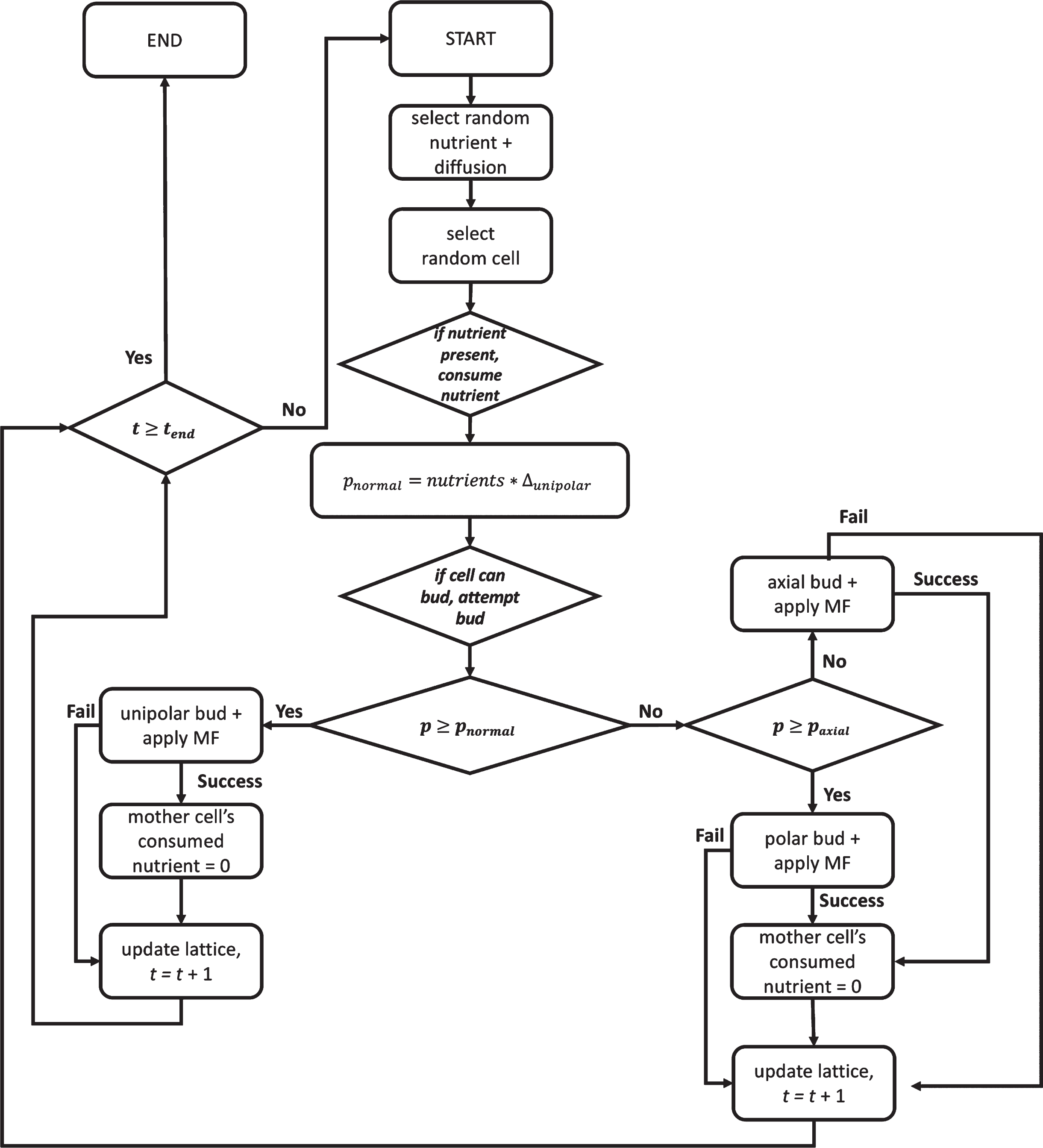
We developed a 2D lattice-based framework to investigate the effects of nutrient conditions and MFs on the growth and morphology of yeast colonies (Fig. 1; see Section 5.1 for algorithmic details). This framework was simulated stochastically to model yeast cells growing in an incubator on agar plates containing different concentrations of nutrients, with or without externally applied MFs [23]. We made the standard assumption that all yeast cells in a colony originate from a single cell and are genetically identical.
Fig. 1
Flow diagram of the lattice algorithm for stochastically simulating the effects of nutrient concentration and magnetic field (MF) exposure on yeast colonies. Rectangles represent a step in the program while diamonds represent an evaluation made of the state of the lattice site to determine the next step to take. pnormal is the probability of the cell budding into an axial or bipolar pattern, rather than the unipolar pattern occurring in low-nutrient conditions. paxial is the probability of the cell budding in an axial pattern. Δunipolar is the fixed amount by which pnormal increases with each nutrient packet consumed. The current timestep is represented by t and tend is the total number of timesteps for which the algorithm is set to run.
When a budding yeast cell prepares for division, it becomes polarized along the mother-bud axis, which determines the direction that the yeast cell will bud [22, 24]. To mimic yeast cell division, bud-site selection in our framework follows one of two patterns: either an axial budding pattern (the primary pattern for haploid yeast cells; Fig. A1A) or the bipolar budding pattern (the primary budding pattern for diploid yeast cells; Fig. A1B) (see Section 5.1.1 for the algorithmic implementation of budding patterns), which can also switch to pseudohyphal growth (Fig. A1C) when nutrients (glucose or nitrogen) are scarce [25]. Pseudohyphal growth in S. cerevisiae is a type of filamentous growth that occurs when elongated ellipsoidal cells that are fully separated by cytokinesis remain attached to each other through proteins and polysaccharides in the cell wall (as opposed to true hyphal growth that occurs in filamentous fungi in which cells fail to undergo cytokinesis and grow as multinucleate hyphae) [25]. Regardless of the budding pattern, the budding direction is determined with respect to the direction of budding in the previous replication, which is marked by a bud scar on the surface of the cell. If a cell has never replicated before, the scar will be at the site at which it separated from its mother cell and is referred to as a birth scar. An axial budding pattern requires that the yeast bud grows adjacent to the bud scar. A bipolar budding pattern is more complex. The daughter cell’s first bud will form at the end furthest from its birth scar. The mother cell’s next bud will form at the end opposite its previous daughter cell, or it may bud at the end closest to its bud scar.
To model the effect of nutrient conditions on the emergent structure of yeast colonies, diploid cells can switch from the bipolar budding pattern to pseudohyphal growth [25] (see Section 5.1.2 for the algorithmic implementation of nutrient conditions). Similarly, in low-nutrient conditions haploid cells can switch to invasive filamentous growth [26–28]. In filamentous growth, new daughter cells are more elongated. These elongated cells will bud along the same direction and do not separate from one another, thus forming chains which resemble the true hyphae seen in other fungi, including pathogenic yeasts [29–31]. Like pseudohyphal growth, invasive growth in haploid cells is a result of cells budding along the same direction.
To implement MFs in our framework, we incorporated the quantitative single-cell MF-budding angle data from Egami et al. [13] (see Section 5.1.3 for the algorithmic implementation of MFs). As there are yet to be experiments performed on the effects of MFs on yeast colony growth and morphology, we assumed that the behavior of a budding yeast colony under static MFs emerges from the division pattern of individual budding yeast cells that make up the colony. Specifically, individual yeast cells were specified to bud within 30° to 150° of the direction of the applied homogeneous static MF (Fig. A2). As this is a 2D model, the direction of the MF was constrained to the same plane as the yeast colony.
For all simulations, unless otherwise indicated, the stopping condition was 320,000 timesteps for time-based simulations and 10,000 cells for cell count-based simulations; for each parameter set and MF condition, simulations were repeated 800 times to generate the statistics and distributions shown in the violin plots (see Section 5.2). Cells were required to consume one nutrient packet to bud and nutrient diffusion was set as a 10-step random walk, which defined a timestep in the simulation [20] (see Section 5.1.4). A single cell in the colony was randomly chosen and analyzed at each time step. The MATLAB code, parameters, and data used to generate the figures presented in this manuscript are available at: https://github.com/CharleboisLab/Yeast-Colony-Models.
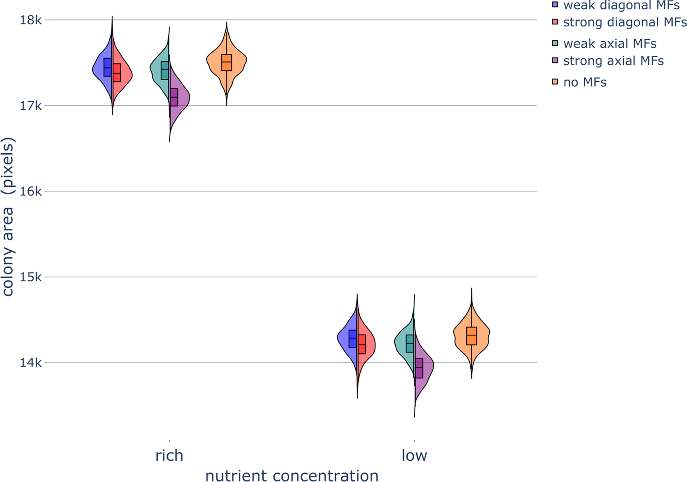
Fig. 2
Haploid colony area under different nutrient and magnetic field conditions. Violin plots of colony area after 320,000 timesteps, when influenced by various magnetic field (MF) directions and strengths under rich-nutrient and low-nutrient conditions. The box and whisker plots within the violin plots denote the median, interquartile range (IQR), and 1.5 × IQR (see Section 5.2 for more details). Simulations were repeated 800 times to generate the violin plots. Parameters were set as follows: rich-nutrient condition: START_NUTRS = 20, low-nutrient condition: START_NUTRS = 2; nSteps = 10; paxial = 0.6; no MFs: MF_STRENGTH = 0, weak MFs: MF_STRENGTH = 0.5, strong MFs: MF_STRENGTH = 1.
3Results and discussion
To computationally investigate the effect of nutrient conditions and MFs on the growth rate and the budding angles of yeast cells, we determined the area, formation time, perimeter, and budding angle distribution of the colonies. The effect of nutrient conditions and MF exposure on colony morphology was quantified by the roundness, elongation, solidity, and boundary fluctuations of the in silico yeast colonies. These quantitative measures are described in Section 5.3.
3.1Low-nutrient conditions
The final colony area decreased as the nutrient concentration decreased (Figs. 2 and A3; Section 5.3.1). This occurred in our simulations as there are fewer nutrient packets diffusing on the lattice in the low-nutrient condition and therefore, on average, cells in the colony consume nutrients at a lower rate and bud less frequently. This result is in agreement with experimental results, where maximum colony area reached a larger size with increasing sugar concentrations (Fig. A3A,C); the in silico colony area saturated at 6 nutrients packets per lattice site (Fig. A3C). Correspondingly, colony perimeter decreased (Fig. A4; Section 5.3.3) and colony formation time increased (Fig. A5; Section 5.3.2) as the nutrient concentration decreased in our simulations. The colony formation time is inversely related to the colony area, meaning that a larger final colony area for a fixed number of timesteps and a smaller number timesteps to reach a given colony size both represent higher growth rates.
Fig. 3
Haploid colony roundness under different nutrient and magnetic field conditions. Violin plots of colony roundness under different nutrient conditions and different magnetic field (MF) directions and strengths. Parameters were set as follows: rich-nutrient condition: START_NUTRS = 20, low-nutrient condition: START_NUTRS = 2; nSteps = 10; paxial = 0.6; no MFs: MF_STRENGTH = 0, weak MFs: MF_STRENGTH = 0.5, strong MFs: MF_STRENGTH = 1, and extra strong MFs: MF_STRENGTH = 2.
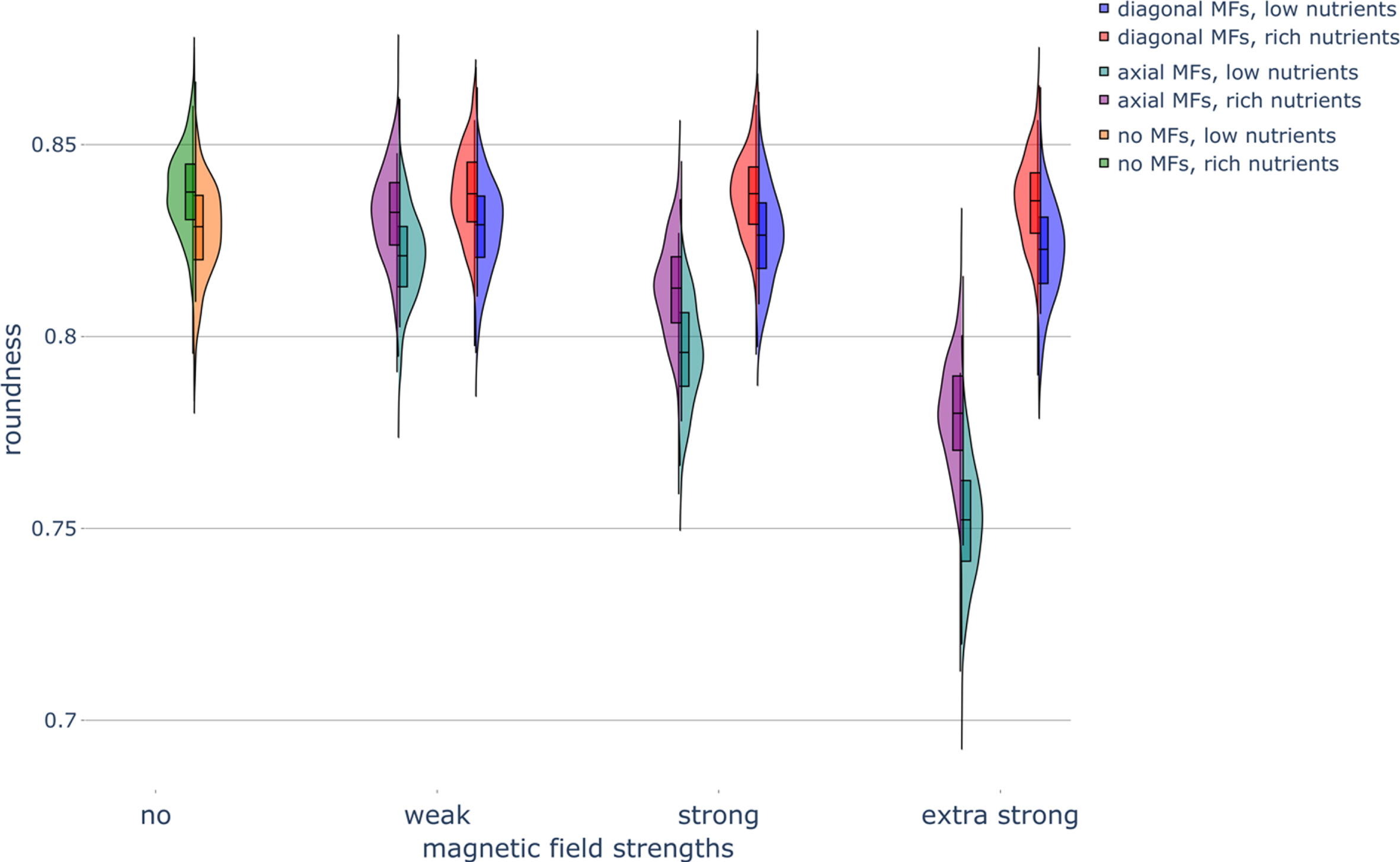
Fig. 4
Haploid colony elongation under different nutrient conditions and magnetic field conditions. Violin plot of colony elongation under various nutrient concentrations and exposure to magnetic fields (MFs) of different strengths and directions. Parameters were set as follows: rich-nutrient condition: START_NUTRS = 20, low-nutrient condition: START_NUTRS = 2; nSteps = 10; paxial = 0.6; no MFs: MF_STRENGTH = 0, weak MFs: MF_STRENGTH = 0.5, strong MFs: MF_STRENGTH = 1, and extra strong MFs: MF_STRENGTH = 2.
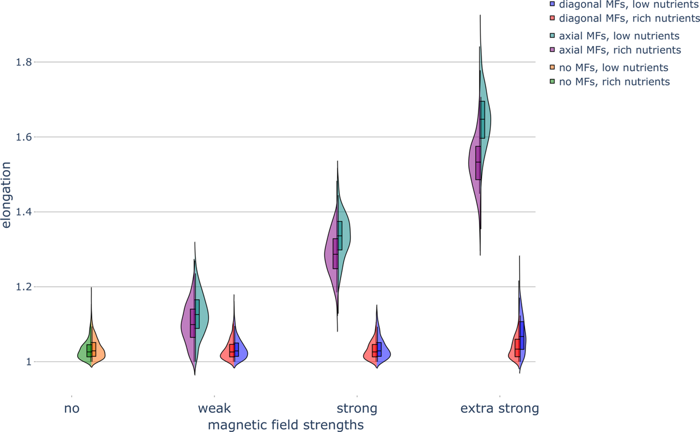
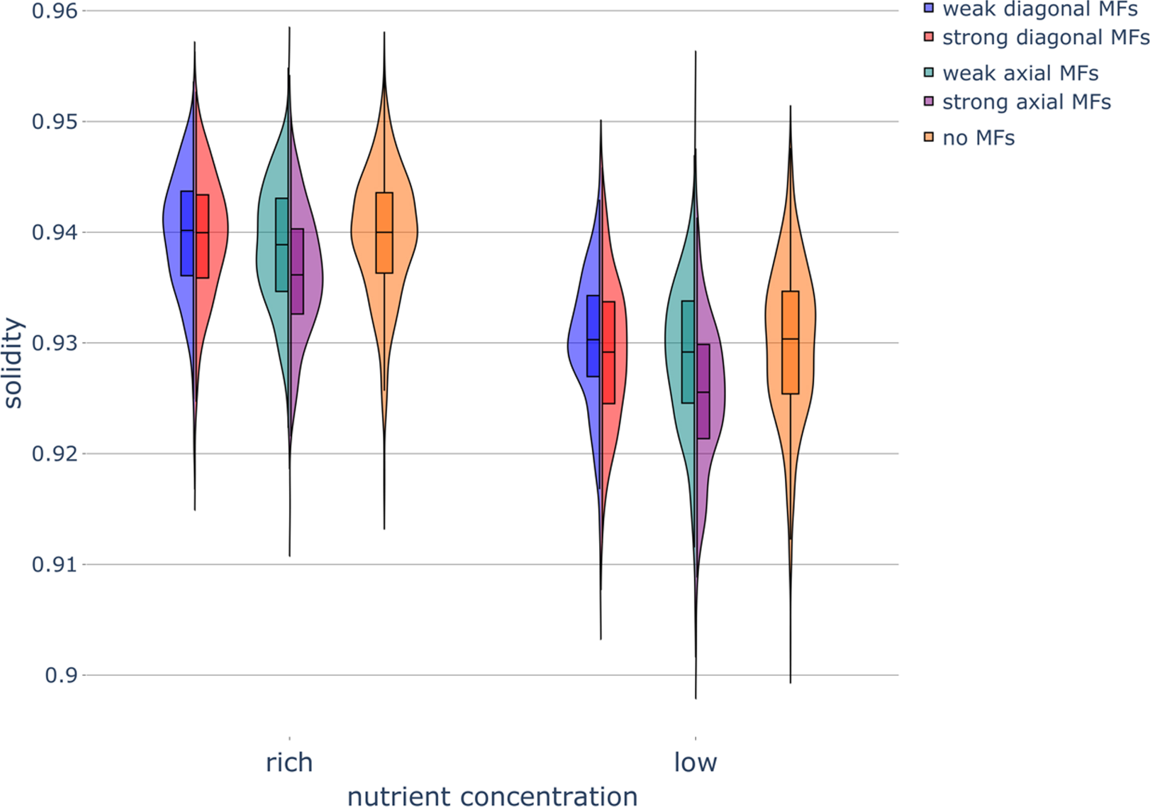
Fig. 5
Haploid colony solidity under different nutrient and magnetic field conditions. Violin plot of colony solidity in various nutrient conditions while exposed to magnetic fields (MFs) of different strengths and directions. Parameters were set as follows: rich-nutrient condition: START_NUTRS = 20, low-nutrient condition: START_NUTRS = 2; nSteps = 10; paxial = 0.6; no MFs: MF_STRENGTH = 0, weak MFs: MF_STRENGTH = 0.5, strong MFs: MF_STRENGTH = 1.
Low-nutrient conditions decrease the roundness of the colonies (Fig. 3; Section 5.3.4). This indicates that the colonies become less circular as nutrient concentrations decrease. When we compared the experimental data from Ref. [13], we found that the P2A measure (Section 5.3.4) increased as the nutrient level decreased (Fig. A3B,D); the in silico P2A stabilized to a minimum value at 6 nutrients packets per lattice site (Fig. A3D). This occurs because yeast cells regularly fail to bud at the colony rim in low-nutrient conditions, resulting in more unoccupied grid lattice sites and a more irregular colony. The decrease in roundness may also be related to petal formation on the colony boundary, which occurs due to increased intercellular competition over low numbers of diffusing nutrients at the colony rim [2]. Nutrient concentration had no effect on colony elongation (Fig. 4). Though elongation and roundness are inversely related, a colony can be less round without being more elongated (but not necessarily vice-versa), as roundness is a more general measure than elongation (see Section 5.3.5).
The solidity of the colonies was found to decrease as the nutrient concentration decreased (Fig. 5). This decrease in solidity can be attributed to the fact that the ability of cells to bud and fill up empty lattice sites in our simulations decreases along with the nutrient concentration.
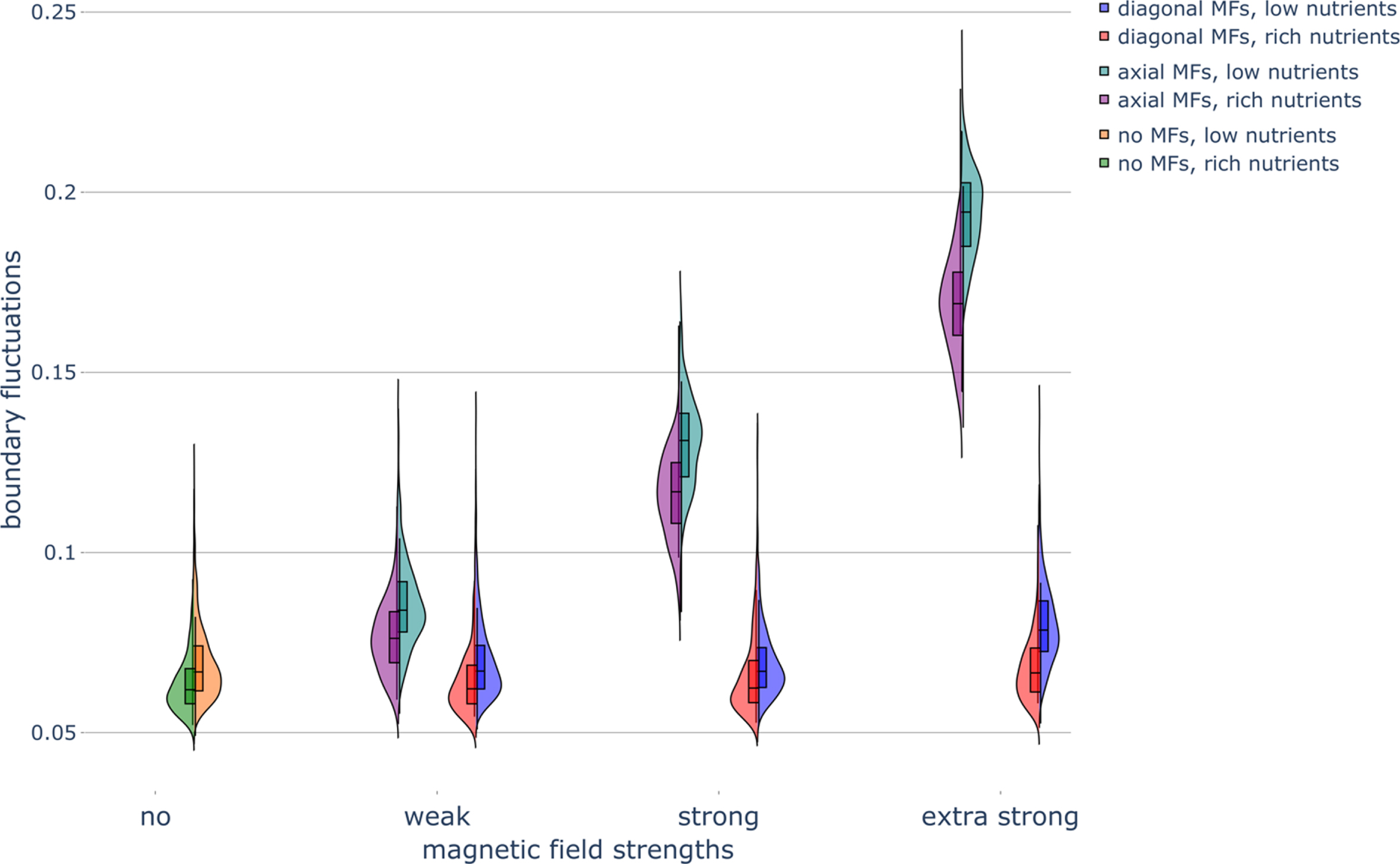
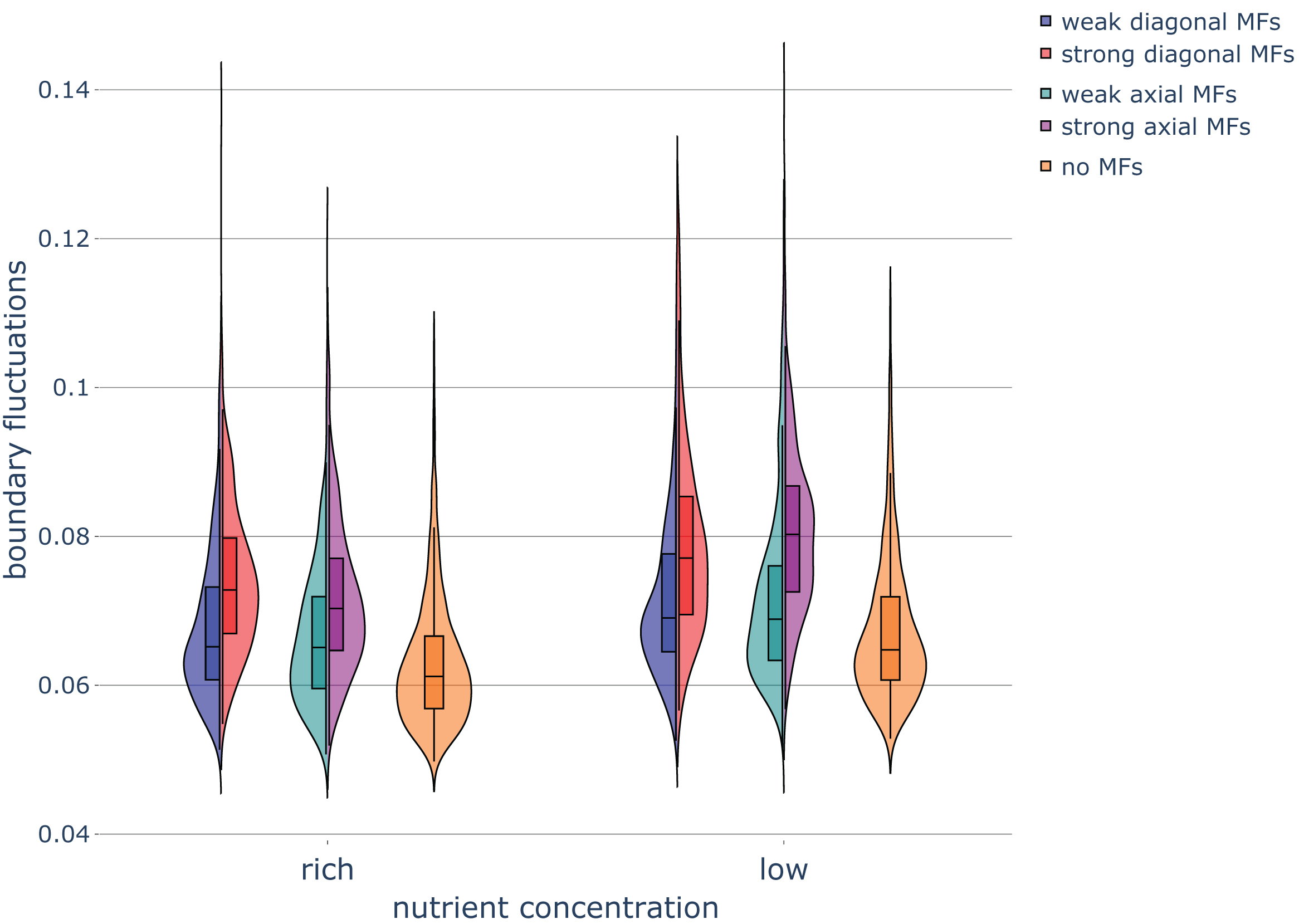
Boundary fluctuations increased as the nutrient concentration decreased (Fig. 6). This increase in irregularity at the colony rim in the low-nutrient condition is in agreement with experimental results (Fig. S5 in Ref. [2]).
Fig. 6
Haploid colony boundary fluctuations under different nutrient and magnetic field conditions. Violin plots of the boundary fluctuations of colonies in various nutrient conditions and exposed to magnetic fields (MFs) of different strengths and directions. Parameters were set as follows: rich-nutrient condition: START_NUTRS = 20, low-nutrient condition: START_NUTRS = 2; nSteps = 10; paxial = 0.6; no MFs: MF_STRENGTH = 0, weak MFs: MF_STRENGTH = 0.5, strong MFs: MF_STRENGTH = 1, and extra strong MFs: MF_STRENGTH = 2.
3.2Magnetic field exposure
We calculated the budding angle each time a cell budded over the course of our simulations. Regardless of ploidy or the nutrient condition, the frequencies of each budding angle for haploid colonies were uniformly distributed when no MF was present, in agreement with experimental results (Fig. A6A). The budding angles in the experimental data had a slight bias towards the 0° to 90° and 270° to 360° angle ranges due to the fact that mother yeast cells tended to orient themselves in the direction of the capillary flow (due to hydrodynamic forces exerted upon the cells) inside the optical magnetic circuit device [13]. When a weak MF was applied, the number of times the budding angle of haploid cells was in the direction of the MF was greater than outside of this range, in agreement with experimental results in the presence of a 2.93T MF (Fig. A6B). This effect was more prominent in our simulations when we applied a strong MF (Fig. A6B). The in silico budding angle distributions were similar for axial MFs and diagonal MFs (data not shown), low-nutrient and high-nutrient conditions (Fig. 7), and for diploid colonies (Fig. A7). Overall, the application of a homogeneous MF in our simulations decreases the variability in the budding process, in agreement with the empirical data.
Fig. 7
Budding angle distributions for haploid colonies under different nutrient conditions and axial magnetic field strengths. Plot of the frequency of the angle between the axial magnetic field (MF) direction and the mother-bud axis. The thick black lines radiating from the center represent the average number of cells that bud in a particular angle. Parameters were set as follows: rich-nutrient condition: START_NUTRS = 20, low-nutrient condition: START_NUTRS = 2; nSteps = 10; paxial = 0.6; MAGNETIC_FIELD = [1 0]; no MFs: MF_STRENGTH = 0, weak MFs: MF_STRENGTH = 0.5, strong MFs: MF_STRENGTH = 1; UNIPOLAR_ON = false.
![Budding angle distributions for haploid colonies under different nutrient conditions and axial magnetic field strengths. Plot of the frequency of the angle between the axial magnetic field (MF) direction and the mother-bud axis. The thick black lines radiating from the center represent the average number of cells that bud in a particular angle. Parameters were set as follows: rich-nutrient condition: START_NUTRS = 20, low-nutrient condition: START_NUTRS = 2; nSteps = 10; paxial = 0.6; MAGNETIC_FIELD = [1 0]; no MFs: MF_STRENGTH = 0, weak MFs: MF_STRENGTH = 0.5, strong MFs: MF_STRENGTH = 1; UNIPOLAR_ON = false.](https://content.iospress.com:443/media/isb/2021/14-3-4/isb-14-3-4-isb210233/isb-14-isb210233-g007.jpg)
The application of a strong axial MF decreased the final colony area independently of the nutrient concentration (Fig. 2). Weak axial and strong diagonal MFs caused a small decrease in the final colony area. Similar results were obtained when the final number of cells in the colony was analyzed instead of the final colony area; axial MFs and strong diagonal MFs increased the number of timesteps required to reach the final colony size (Fig. A5). Axial MFs decreased the solidity of colonies slightly, with strong axial MFs having a more pronounced effect than weak axial MFs (Fig. 5); diagonal MFs had no effect on colony solidity.
Interestingly, MFs had little effect on the colony perimeter regardless of the nutrient condition (Fig. A4). The lack of an effect of MFs on colony perimeter can be attributed to the fact that the perimeter is also influenced by irregularities at the colony boundary, which are more accurately determined from the boundary fluctuation measurement (Section 5.3.7). Namely, if boundary fluctuations were not a factor, a decrease in colony area in the presence of a MF (Fig. 2) would lead to a decrease in colony perimeter. On the other hand, if colony area was not a factor, the increase in boundary fluctuations when exposed to MFs (Fig. 6), would cause an increase in colony area. Since both colony area and boundary fluctuation effects are present, these opposing influences on perimeter cancel each other out. Axial MFs caused a large increase in the boundary fluctuations, with strong axial MFs causing an even larger increase than weak axial MFs. Though diagonal MFs did not affect boundary fluctuations, extra strong diagonal MFs increased boundary fluctuations, particularly in the low-nutrient condition (Fig. 6).
Strong axial MFs decreased the roundness of the colonies regardless of the nutrient concentration; this effect was even more pronounced for extra-strong axial MFs (Fig. 3). Weak axial MFs had little effect on colony roundness. The application of axial MFs greatly increased the elongation of the colonies, with strong axial MFs having an even greater effect than weak axial MFs (Fig. 4). Therefore, the exposure of budding yeast cells to axial MFs is predicted to generate less circular colonies, in agreement with colony roundness results (Fig. 3). Diagonal MFs had no effect on roundness (Fig. 3) or the elongation of colonies (Fig. 4), also in agreement with the colony roundness results. However, diagonal MFs did begin to have an effect in low nutrient conditions, like with boundary fluctuations, increasing the elongation of colonies when the strength of the MF was increased to the extra strong condition (Fig. 4). Extra strong axial MFs also displayed an increased effect compared to strong axial MFs. Finally, the application of axial MFs substantially increased the haploid colony-to-colony variability in boundary fluctuations (Fig. 6) as well as in elongation (Fig. 4).
Overall, though strong axial MFs and low-nutrient conditions both reduced colony growth, the nutrient condition is predicted to have a greater effect on the growth rate of the colony compared to the application of MFs. Together, these results suggest that nutrient limitation in the microenvironment and MF exposure could be used to mitigate growth in yeast infections and colony biofilms, and provide a novel way to control the morphology of cells growing on biomaterials.
3.3Ploidy dependent magnetic field effects
To investigate why axial MFs had a greater overall effect than diagonal MFs on the growth and morphology of haploid yeast colonies, we performed the corresponding simulations on diploid yeast cells. As opposed to axial budding pattern in haploid colonies, diploids follow a bipolar budding pattern (Fig. A1B) when nutrients are abundant and switch to filamentous growth (Fig. A1C) when nutrients are scarce [25].
In the absence of MFs and pseudohyphal growth, diploid colonies reached a larger final area than haploid colonies (Fig. 8); this effect was also reflected in the shorter times for diploid colonies to reach 10,000 cells (Fig. A10) and in larger diploid colony perimeters (Fig. A11), when compared to haploid colonies (Figs. 2, A4, and A5). We attribute the larger size of the diploid colonies compared to haploid colonies in our simulations to differences in their respective budding patterns. Diploids may have a higher success rate for budding because of less crowding in the surrounding lattice sites, resulting from budding switching between the different poles of diploid cells.
Fig. 8
Colony area of haploid and diploid colonies without filamentous growth under different nutrient concentrations. Violin plots of yeast colony area after 320,000 timesteps for different ploidies under rich-nutrient and low-nutrient concentrations with diffusion and no magnetic fields (MFs). Parameters were set as follows: rich-nutrient condition: START_NUTRS = 20, low-nutrient condition: START_NUTRS = 2; nSteps = 10; haploid: paxial = 0.6, diploid: paxial = 0; MF_STRENGTH = 0.
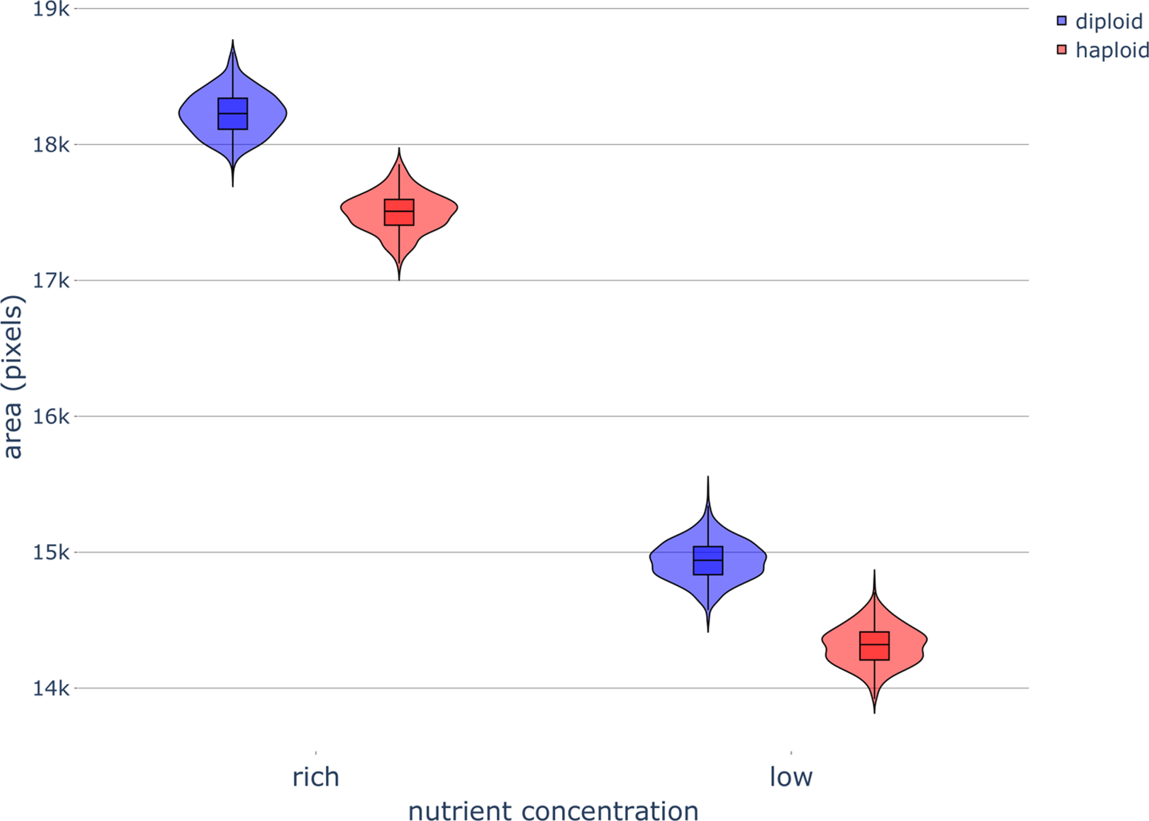
Fig. 10
Elongation of diploid colonies without pseudohyphal growth under different nutrient conditions and applied magnetic fields. Violin plot of colony elongation under various nutrient concentrations and exposure to magnetic fields (MFs) of different strengths and directions. Parameters were set as follows: rich-nutrient condition: START_NUTRS = 20, low-nutrient condition: START_NUTRS = 2; nSteps = 10; paxial = 0; no MFs: MF_STRENGTH = 0, weak MFs: MF_STRENGTH = 0.5, strong MFs: MF_STRENGTH = 1.
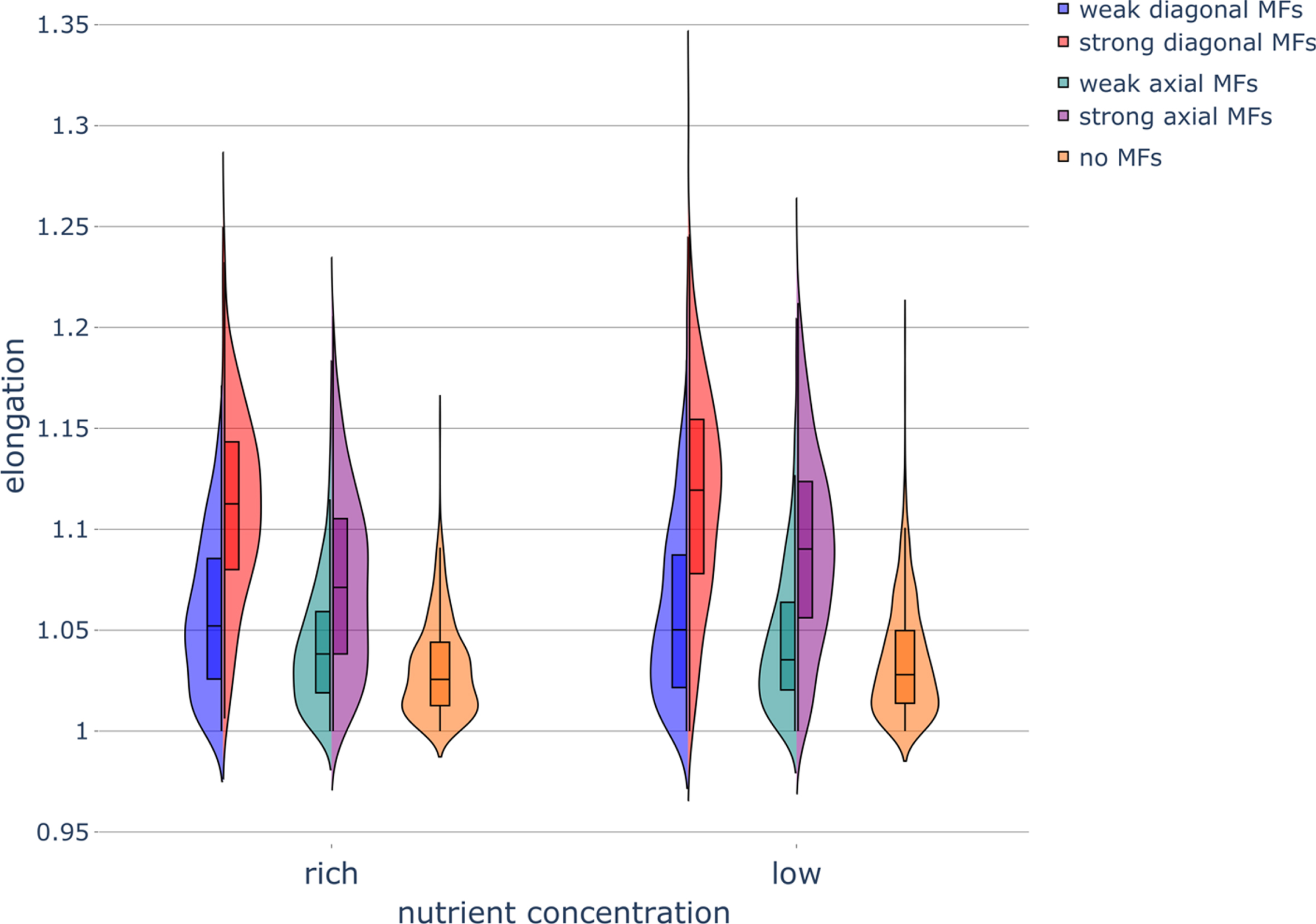
Fig. 11
Boundary fluctuations of diploid colonies without pseudohyphal growth under different nutrient and magnetic field conditions. Violin plots of the boundary fluctuations of colonies in various nutrient conditions and exposed to magnetic fields (MFs) of different strengths and directions. Parameters were set as follows: rich-nutrient condition: START_NUTRS = 20, low-nutrient condition: START_NUTRS = 2; nSteps = 10; paxial = 0; no MFs: MF_STRENGTH = 0, weak MFs: MF_STRENGTH = 0.5, strong MFs: MF_STRENGTH = 1.
For haploid colonies undergoing invasive growth, axial MFs and diagonal MFs had a substantial effect on colony morphology, resulting in horizontally or diagonally stretched colonies, respectively, particularly in the low-nutrient condition (Fig. 9). Diploid colonies that could switch to pseudohyphal growth had a lower cell count at the end of the simulations in the low-nutrient condition (on average 7,500 cells in the low-nutrient condition compared to on average 11,500 cells in the nutrient-rich condition), in agreement with the nutrient-dependent growth results for haploid yeast colonies (Figs. 2 and 9). Haploid colonies (Fig. 9) and diploid colonies (data not shown) were less dense under nutrient limitation and MF exposure as result of these colonies containing more holes (i.e., unoccupied lattice sites); diploid colonies were found to be less solid in the low-nutrient condition (Fig. A13). Diagonal MFs resulted in more elongated diploid colonies when there was no pseudohyphal growth (Fig. 10) compared to haploid colonies whose elongation was not influenced by weak or strong diagonal MFs (Fig. 4). Diagonal MFs also increased the boundary fluctuations in diploid colonies (Fig. 11) compared to haploid colonies, whose boundary fluctuations were not influenced by weak or strong diagonal MFs (Fig. 4). The application of axial and diagonal MFs substantially increased the diploid colony-to-colony variability in elongation (Fig. 10) and boundary fluctuations (Fig. 11).
Fig. 9
Visual representation of simulated haploid colonies with filamentous growth under different nutrient and magnetic field (MF) conditions. Parameters were set as follows: rich-nutrient condition: START_NUTRS = 20, low-nutrient condition: START_NUTRS = 2; nSteps = 10; paxial = 0; diagonal MF direction: MAGNETIC_FIELD = [1 1], axial MF direction: MAGNETIC_FIELD = [1 0]; no MFs: MF_STRENGTH = 0, weak MFs: MF_STRENGTH = 0.5, strong MFs: MF_STRENGTH = 1; UNIPOLAR_ON = true.
![Visual representation of simulated haploid colonies with filamentous growth under different nutrient and magnetic field (MF) conditions. Parameters were set as follows: rich-nutrient condition: START_NUTRS = 20, low-nutrient condition: START_NUTRS = 2; nSteps = 10; paxial = 0; diagonal MF direction: MAGNETIC_FIELD = [1 1], axial MF direction: MAGNETIC_FIELD = [1 0]; no MFs: MF_STRENGTH = 0, weak MFs: MF_STRENGTH = 0.5, strong MFs: MF_STRENGTH = 1; UNIPOLAR_ON = true.](https://content.iospress.com:443/media/isb/2021/14-3-4/isb-14-3-4-isb210233/isb-14-isb210233-g009.jpg)
In summary, these results indicate that the interaction between MFs and ploidy-dependent budding patterns determines if an applied axial MF or diagonal MF will yield the greatest effect on colony growth and morphology. This is important because a nutrient- and MF-dependent decrease in solidity could in principle reduce antimicrobial resistance in colony biofilms by enhancing the penetration of antimicrobial drugs.
4Conclusion
We developed a 2D Monte Carlo lattice-based simulation framework to spatiotemporally investigate the interplay between biochemical phenomena and physical forces in yeast. This novel computational framework was able to reproduce experimental results obtained under nutrient-varying conditions [2]. The simulated budding angle distributions were also found to be in agreement with experimental budding angle distributions under magnetic field exposure [13]. The framework was then used to make novel predictions on the effects of magnetic fields on colony growth and morphology.
Monte Carlo simulation of the framework accurately captured the colony area and colony formation time in agreement with previous experiments on budding yeast [2]. This was achieved by modeling the diffusion of nutrient molecules that cells on the lattice consumed to divide. The nutrient packets could be replaced with drug molecules to model drug delivery and the formation of drug-resistant biofilms. We anticipate that this framework will also be suitable for modelling clonal interference among drug-resistant mutants [32] and that it could be expanded to three dimensions to model the invasive growth (i.e., the vertical penetration of the filaments into the agar or tissue) of haploid yeast cells exposed to nutrient-limiting conditions [26–28], as well as more intricate pattern formation in eukaryotic biofilms [2]. Augmenting the framework to incorporate additional details such as the occasional budding of daughter cells adjacent to their bud scars [22, 33] and more complex yeast behaviors, including mating between haploid cells, and meiosis and sporulation in diploid cells facing extreme nutrient-depletion conditions [34–36], will be important areas to explore in future work.
The Monte Carlo lattice-based framework was used to generated novel predictions on how magnetic fields affect the emergent growth and morphological properties of yeast colonies by incorporating experimental data on the budding angle of individual yeast cells exposed to magnetic fields [13]. Strong magnetic fields were shown in our simulations to exhibit wide-ranging effects on yeast colony growth and morphology in low-nutrient and high-nutrient conditions. The decrease in colony growth rate due to applied magnetic fields opens the possibility of using electromagnetic fields to control fungal infections and mitigate biofilm formation. Similarly, the decrease in colony solidity under magnetic field exposure may increase the ability of antimicrobial drugs to penetrate biofilms when they are exposed to electromagnetic fields. Finally, the elongation of the colonies along the magnetic field vector in our simulations may provide a novel way to control cellular growth on biomaterials.
Comparison between haploid and diploid colony simulations revealed that the interaction between the magnetic field and the budding pattern determines if an applied axial or diagonal magnetic field will yield the greatest effect on colony growth and morphology. Overall, axial magnetic fields affected haploid and diploid colonies, whereas diagonal magnetic fields had a greater effect on diploid colonies; extra-strong diagonal magnetic fields also affected haploid colonies. The differences between the implementation of the axial and diagonal magnetic fields in our simulations are a limitation of using a square lattice and not a true electromagnetic phenomenon. This may be resolved in future work by using a hexagonal mesh rather than a square lattice [37–39]. Electromagnetic fields have also been observed to affect yeast cell proliferation in a frequency-dependent manner [12], which could be simulated using the framework by incorporating alternating magnetic fields. The mechanism by which budding yeast cells orient themselves to magnetic fields is an open question, though it has been hypothesized to be a result of polarized microtubules [13]. Further experiments on yeast cells are required to validate our magnetic field simulation results and to elucidate the mechanisms underlying these biomagnetic effects.
The budding patterns in our framework are specific to haploid and diploid budding yeast cells. Though these details render the nutrient-limiting and magnetic field simulations unique and biologically relevant, the trade-off is that it limits the applicability of the model to other microorganisms, cell types, tissues, and so forth. One way to address this limitation is to modify the yeast-specific budding pattern into general cell division rules that are more broadly applicable to other organisms. Another limitation of our model is that it does not account for the morphological details of single cells. Using a hexagonal lattice [37–39] or an off-lattice [40, 41] approach would help resolve this issue, though these approaches are not without their own limitations. For instance, using a hexagonal lattice would decrease the budding angle resolution (as there are 6 neighbors, instead of 8 neighbors on a square lattice), which would make it more difficult to distinguish between ploidy-dependent and magnetic field-dependent effects. An off-lattice implementation of the model would have a higher resolution in terms of budding angle (as any budding angle could be used), which would more accurately model elongation (e.g., for invasive pseudohyphal or hyphal growth) and could capture the dynamics of the mother cell while budding. However, an off-lattice approach would be more computationally intensive than a square or hexagonal implementation of the model.
Quantitative spatiotemporal modelling, such as the Monte Carlo lattice-based framework presented in this study, combined with the development of electromagnetic devices to perform controlled laboratory experiments will provide powerful tools for elucidating bioelectromagnetic mechanisms in microbial communities. Uncovering such mechanisms may one day allow electromagnetic fields to be used to control growth and biofilm formation in yeast and other microorganisms including magnetotactic bacteria [42], as well as to enhance the efficacy of antimicrobial drugs.
5Methods
5.1Lattice-based framework
5.1.1Algorithmic implementation of budding patterns
The MF bias rules were based on experimental data that showed that the angle between the mother-bud axis and the direction of the MF was most often between 30° to 150° and –30° to –150° [13].
In our computational model, the bud (or birth) scar of each cell is represented by a vector, [x, y]. This vector indicates the direction of polarization by the difference in coordinates between the cell and its previous bud (or in the case of a daughter’s birth scar, its mother cell). If the coordinates of a cell are (x, y) and it produces a bud at coordinates (x′, y′), then the cell’s bud scar is given by [x-x′, y-y′] and the new bud’s birth scar will be the opposite, [x′-x, y′-y]. This model uses a “Moore neighborhood”, meaning that all eight lattice sites surrounding a cell are considered possible sites into which a cell can bud [43]. If all eight sites are occupied by cells, the surrounding area is considered too crowded, and the cell cannot bud. The angle assigned to a neighboring site at (x′, y′) of a cell at (x, y) with bud scar [a, b] is given by the angle between the vector [x′-x, y′-y] and [a, b].
To model axial budding, the angles between a cell’s bud scar and each empty lattice site surrounding it are calculated (Fig. A1A). We observed that if the smallest angle is chosen as the direction of budding, and in the case where one of two empty sites with the same smallest angle is chosen randomly, that diamond-shaped colonies are produced (data not shown); diamond-shaped colonies do not resemble the circular colonies commonly grown on agar plates in the laboratory [23]. To rectify this, budding is restricted to the two sites 45° from the bud scar (Fig. A1A). If both adjacent sites are empty, one site is chosen randomly. If only one site is empty, the cell will bud into the empty site. If both adjacent sites are occupied, the cell will randomly bud into one of the two sites, pushing the occupying cell into a randomly selected empty site nearby. As before, if there are no empty sites around the occupying cell, then the area is considered too crowded, and the cell will not be able to bud. The resulting simulations yielded approximately circular colonies in rich-nutrient conditions and in the absence of MFs (Fig. 9), in agreement with standard experimental observations (e.g., [2, 23]). This effect, as well as the length over which a cell can push neighbor cells away, has been previously described in cellular automata with one cell per lattice site [44–46].
Bipolar budding (Fig. A1B) is modeled as a combination of two sets of budding rules. The new bud will either form near the bud scar, in which case the same rules as those used for axial budding are used (Fig. A1B, Case 2); otherwise, the bud site will be on the end opposite to the previous bud scar, in which case polar budding rules are specified (Fig. A1B, Case 1). According to the polar budding rules, the cell can bud into the sites which are either 135° or 180° from the bud scar. If multiple sites are available, then one is randomly selected. If none of these sites are available, then one is randomly selected and the occupying cell is pushed out of the way, unless that area of the colony is considered too crowded, in which case the cell cannot bud. The polar and axial budding rules are used together to simulate the bipolar budding pattern of diploid cells. How often a cell buds at the distal pole, as opposed to the proximal pole, is affected by several factors [33]. For simplicity, in our model the bipolar budding pattern is set to follow axial budding rules half of the time and polar budding rules the other half of the time. The only exception to this rule is when a cell divides for the first time, in which case it will always bud according to the polar rules when budding in a bipolar pattern.
A parameter is set at the beginning of the simulation to indicate what fraction of cells will bud axially (paxial). In a typical haploid colony 60–75% of cells will bud along an axial pattern and 20–40% of cells will bud in a bipolar pattern, while the remaining percentage of cells will bud randomly [47]. A paxial of 60% was used in our model for the haploid colonies. In a typical diploid colony, nearly all cells bud according to the bipolar pattern, with occasional random budding; in this case a paxial of 0% was used. Whenever a cell attempts to a bud, a random number between 0 and 1 is generated from a uniform distribution. If this random number is less than paxial, the cell will bud axially, otherwise the cell will bud in a bipolar fashion.
5.1.2Algorithmic implementation of nutrient conditions
Nutrient concentrations were modelled using discrete nutrient packets. Three parameters related to nutrients are set at the beginning of the simulation. The first parameter is nSteps, the length of the random walk taken by a diffusing nutrient packet. The second parameter is START_NUTRS, the initial nutrient concentration, which sets the number of nutrient packets that will be uniformly distributed across the lattice at the beginning of each simulation (e.g., for the low-nutrient condition, there are initially two nutrient packets at each unoccupied lattice site). The third parameter is NUTRS_FOR_BUDDING, the number of nutrient packets that a cell must consume before it can bud. For each simulation step, a random lattice site containing at least one nutrient packet is selected (Fig. 1). This nutrient packet then takes a random walk of nSteps across the lattice. After a nutrient packet moves, a random cell is selected. If at least one nutrient packet is present at this cell’s location, it will be consumed. If this cell has consumed NUTRS_FOR_BUDDING packets, it will attempt to bud according to the budding rules described above.
To model pseudohyphal growth in low-nutrient conditions, we incorporated a unipolar budding condition (Fig. A1C). The frequency of a cell budding according to this growth pattern is tied to the number of nutrient packets at the site occupied by a cell. Before any budding occurs, the probability that the selected cell will not bud according to the unipolar budding rules is calculated as the number of nutrient packets at that lattice site multiplied by a parameter Δunipolar. This parameter is the reciprocal of 8 (the number of lattice sites surrounding a cell) times the number of nutrients a cell must consume to bud (NUTRS_FOR_BUDDING). Therefore, if there are 8*Δunipolar nutrient packets, then there are exactly enough nutrients for the cell to bud into all 8 lattice sites; this is the threshold for the high-nutrient concentration. At this level of nutrients and above, the probability of budding in a normal budding pattern (pnormal) is 1. If the level of nutrients is below this threshold, then there is a chance that unipolar budding (i.e., invasive or pseudohyphal filamentous growth) may occur. When a cell attempts to bud, a random number is generated from a uniform distribution between 0 and 1. If it is lower than pnormal, the cell will bud normally, and if it is higher than pnormal, it will grow according to the unipolar budding pattern. The lower the number of nutrient packets, the smaller the fraction and therefore the higher the chance of filamentous growth. If the initial nutrient concentration at every lattice site is sufficiently high, the simulation emulates the standard culture condition. When a cell buds according to the unipolar budding rules, the bud will occupy two lattice sites, one in front of the other along the mother-bud axis to create an elongated cell (Fig. A1C). The mother cell’s bud scar will remain the same, rather than changing according to the direction of budding. This keeps the direction of future budding the same, simulating how cells bud in a chain in the same direction when undergoing filamentous growth. The lattice site representing the tip of the elongated cell has a bud scar set to be in the direction towards the mother cell, while the site closer to the mother cell has a bud scar of [0 0], such that it will not be able to bud. This occurs because this site represents the tail end of the elongated daughter cell, which is still attached to its mother cell, so nothing can bud from this end. Since filamentous growth primarily involves chains of cells that do not fully detach from each other, the unipolar budding condition cannot push other cells out of the way since cells do not bud in the middle of the chain. This limits the amount of unipolar budding that occurs in the middle of the colony, which represents actual colony growth more accurately: pseudohyphal growth in low-nutrient conditions occurs primarily at the colony edge to permit cells to search for nutrients [29, 30]. In the simulations, the parameter UNIPOLAR_ON controls whether cells will switch to unipolar budding in low nutrient conditions. If this parameter is false, cells will bud according to the normal budding rules regardless of the nutrient concentration.
5.1.3Algorithmic implementation of magnetic fields
Whenever a cell buds in the presence of a MF, a MF bias condition is applied (Fig. A2). If a cell buds and pushes another cell out of the way, the direction in which that cell is pushed will also be biased in the direction of the MF vector (
The parameter MF_STRENGTH was introduced to control the strength of the MF. Each time the function for the MF bias is called (Fig. 1), a uniformly distributed random number between 0 and 1 is generated. If this number is less than the threshold set by MF_STRENGTH, then the bias condition will be applied, otherwise it will not be applied. A strong MF is set when MF_STRENGTH is equal to 1, in which case the MF bias condition is applied every time. The model prioritizes budding into an empty site over budding along the direction of the MF, so in the case that the only unoccupied sites around the cell are outside of the space preferred by the MF (grey sites in Fig. A2), the cell will bud into those empty sites. An extra strong MF bias condition was created as well. The extra strong MF behaves similarly to the regular MF bias, except in the case when all the sites around the cell in the space preferred by the MF are occupied and there are unoccupied sites outside of this space. While in the normal MF bias condition, the cell would simply bud into one of those empty sites, the extra strong MF forces the cell to bud into a site in the preferred space and push the occupying cell out of the way. The extra strong MF condition can be applied by setting MF_STRENGTH to any number greater than 1.
5.1.4Simulation Timestep
In our simulation framework, a timestep (tstep) is defined as the time for a nutrient packet to complete a 10-step random walk, which was based on a previous study [20]. The mean displacement of a 2D-random walk is described by [48]:
(1)
(2)
(3)
(4)
The time to culture S. cerevisiae colonies on agar plates under standard laboratory conditions is 2-3 days [23].
5.2Violin plots
Violin plots were chosen to represent our simulation data as they are more informative compared to box whisker plots alone. Violin plots show the full distribution of the data in addition to the box and whisker plots that they contain (Fig. A15). The box and whisker plots show the following summary statistics: interquartile range (IQR: box from the first to the third quartile), median (vertical line through the box), and ±1.5 × IQR (lines or “whiskers” emanating from each quartile). For the sake of visual clarity, our box and whisker plots exclude outliers. The curve represents the distribution of data for a particular quantity (e.g., colony area in Fig. 2). The width of the histogram captures the colony-to-colony uncertainty in each quantity for a given nutrient-MF condition.
5.3Quantitative colony measures
5.3.1Colony area
The area of the in-silico colonies was determined using MATLAB’s bwarea function, giving roughly the number of pixels of the final colony image.
5.3.2Colony formation time
Colony formation time was calculated in the simulations as the time necessary for colonies to reach 10,000 cells.
5.3.3Colony perimeter
The perimeter of the colony was determined from a list of coordinates of the boundary pixels; a sum of the distance from each pixel to the next on the colony edge was obtained from these coordinates.
5.3.4Colony roundness
Roundness is the ratio of the area of the colony to the area of a circle having the same perimeter as the “convex hull” of the colony:
(5)
5.3.5Colony elongation
Elongation is the ratio of the width to the height of the bounding box of an in-silico colony; a higher ratio increases indicates a more elongated colony. The bounding box of the colony image is the smallest possible rectangle which contains the entire area of the colony. This was determined by finding the angle of orientation of the colony with the orientation property of the regionprops function in MATLAB and then using this to orient the colony along the y-axis, before applying regionprops to find the bounding box property. It was necessary to orientate the colony along the y-axis as the bounding box property only finds the smallest possible rectangle which is not rotated. By rotating the colony, colonies that were stretched in any direction could be compared without the direction of elongation influencing the results.
Colony elongation and colony roundness (Section 5.3.4) are related; the more elongated a colony is the less round it is. However, a colony can be less round without being more elongated, as roundness is a more general measure than elongation. This can be seen by the fact that nutrient concentration does not affect colony elongation (Figs. 4 and 10) but does affect colony roundness (Figs. 3 and A12). This indicates that nutrient concentration does not cause the colony to stretch out along a given direction, but rather makes the colony shape more irregular in general, reflecting coarse irregularities in the boundary (see Section 5.3.7). On the other hand, when a MF influences both roundness and elongation the effect is inversely correlated; when elongation is increased by a MF (Fig. 4), colony roundness is decreased by the same MF (Fig. 3).
5.3.6Colony solidity
Solidity is the ratio of the area of the colony to the area of the convex hull:
(6)
5.3.7Boundary fluctuations
The boundary fluctuation measure captures irregularities in the colony shape, such as petals and asymmetries that form at the colony rim. Specifically, the boundary fluctuation is the ratio of the standard deviation of the normalized radial lengths (σRL) to the mean normalized radial lengths (μRL):
(7)
The radial length is the distance from the center of the colony to a point on the boundary; the centroid was calculated using the regionprops function in MATLAB. Each radial length is normalized by dividing it by the maximum radial length.
Boundary fluctuations are not related to colony elongation (Section 5.3.5). Elongation refers to how stretched a colony is, whereas boundary fluctuations refer to and are sensitive to irregularities along the rim of the colony. Similarly, colony roundness (Section 5.3.4) is not sensitive to small irregularities, but rather coarse irregularities along the colony boundary due to its definition in terms of the convex perimeter rather than the perimeter. For instance, weak axial MFs affect boundary fluctuations (Fig. 6) but not roundness (Fig. 3). This indicates that small fluctuations along the colony boundary due to an increase in MF strength make the colony boundary more irregular, as opposed to making the shape of the colony more irregular.
Acknowledgments
DC was supported by funding from an NSERC Discovery Grant (RGPIN-2020-04007), an NSERC Discovery Launch Supplement (DGECR-2020-00197), and the University of Alberta. RH was supported by a 2020 Alberta Innovates Summer Research Studentship and a 2021 NSERC Undergraduate Student Research Award.
The authors thank Akila Bandara, Lesia Guinn, and Prof. Jay Newby for helpful discussions and Harold Flohr for assistance with Fig. A14. We would also like to thank Prof. Gábor Balázsi for providing us with the experimental data from Chen et al., PLoS Computational Biology, 2014. Finally, we acknowledge the two anonymous reviewers whose critical reading of the manuscript and insightful comments helped improve and clarify the manuscript.
Author contributions
DC conceptualized and supervised the study. RH and DC developed the lattice-based modeling framework. RH developed the MATLAB code and performed the simulations. DC benchmarked the framework against experimental data. RH and DC analyzed the results. DC and RH wrote the manuscript.
SUPPLEMENTARY MATERIAL
[1] The Appendix containing the supplementary figures is available in the electronic version of this article: https://dx.doi.org/10.3233/ISB-210233.
REFERENCES
[1] | Palková Z. , Váchová L. , Life within a community:benefit to yeast long-term survival, FEMS Microbiol Rev 30: ((2006) ), 806–824. |
[2] | Chen L. , et al., Two-Dimensionality of Yeast Colony Expansion Accompanied by Pattern Formation, PLoS Comput Biol 10: ((2014) ), e1003979. |
[3] | Nikolaev Y.A. , Plakunov V.K. , Biofilm—“City of Microbes” or an Analogue of Multicellular Organisms? Microbiology 76: ((2007) ), 125–138. |
[4] | Donlan R.M. , Biofilms: microbial life on surfaces, Emerg Infect Dis 8: (9) ((2002) ), 881–890. |
[5] | Kojic E.M. , Darouiche R.O. , Candida infections of medical devices, Clin Microbiol Rev 17: ((2004) ), 255–267. |
[6] | Ramage G. , et al., Candida biofilms: an update, Eukaryot Cell 4: ((2005) ), 633–638. |
[7] | Hing K.A. , Biomaterials - where biology, physics, chemistry, engineering and medicine meet, Journal of Physics Conference Series 105: ((2008) ), 012010. |
[8] | Binninger D.M. , Ungvichian V. , Effects of 60Hz AC magnetic fields on gene expression following exposure over multiple cell generations using Saccharomyces cerevisiae, Bioelectrochem Bioenerg 43: ((1997) ), 83–89. |
[9] | Ikehata M. , et al., Effects of intense magnetic fields on sedimentation pattern and gene expression profile in budding yeast, J Appl Phys 93: ((2005) ), 6724–6726. |
[10] | Novak J. , et al., Effects of low-frequency magnetic fields on the viability of yeast Saccharomyces cerevisiae, Bioelectrochemistry 70: ((2007) ), 115–121. |
[11] | Kthiri A. , et al., Biochemical and biomolecular effects induced by a static magnetic field in Saccharomyces cerevisiae: Evidence for oxidative stress, PLOS ONE 14: (1) ((2019) ), e0209843. |
[12] | Barabáš J. , Radil R. , Malíková I. , Modificationof S. cerevisiae Growth Dynamics Using Low Frequency ElectromagneticFields in the 1-2kHz Range, BioMed Res Int 2015: ((2015) ), 694713. |
[13] | Egami S. , Naruse Y. , Watarai H. , Effect of static magnetic fields on the budding of yeast cells, Bioelectromagnetics 31: ((2010) ), 622–629. |
[14] | Van Liedekerke P. , et al., Simulating tissue mechanics with agent-based models: concepts, perspectives and some novel results, Comptutational Particle Mechanics 2: ((2015) ), 401–444. |
[15] | Ising E. , Beitrag zur Theorie des Ferromagnetismus, Z Physik 31: ((1925) ), 253–258. |
[16] | Lau K.F. , Dill K.A. , A lattice statistical mechanics model of the conformational and sequence spaces of proteins, Macromolecules 22: ((1989) ), 3986–3997. |
[17] | Dubey S.P.N. , et al., A review of protein structure prediction using lattice model, Crit Rev Biomed Eng 46: ((2018) ), 147–162. |
[18] | Ermentrout G.B. , Edelstein-Keshet L. , Cellular Automata Approaches to Biological Modeling, J Theor Biol 160: ((1993) ), 97–133. |
[19] | Hatzikirou H. , Deutsch A. , Cellular automata as microscopic models of cell migration in heterogeneous environments, Curr Top Dev Biol 81: ((2008) ), 401–434. |
[20] | Matsuura S. , Random Growth of Fungal Colony Model on Diffusive and Non-Diffusive Media, Froma 15: ((2000) ), 309–319. |
[21] | Tronnolone H. , et al., Diffusion-limited growth of microbial colonies, Scientific Reports 8: ((2018) ), 5992. |
[22] | Chiou J.-g. , Balasubramanian M.K. , Lew D.J. , Cell Polarity in Yeast, Annu Rev Cell Dev Biol 33: ((2017) ), 77–101. |
[23] | Green S.R. , Moehle C.M. , Media and culture of yeast, Curr Protoc Cell Biol 4: ((1999) ), 1.6.1–1.6.12. |
[24] | Chant J. , Cell polarity in yeast, Trends Genet 10: ((1994) ), 328–333. |
[25] | Cullen P.J. , Sprague G.F.J. , The Regulation of Filamentous Growth in Yeast, Genetics 190: (1) ((2012) ), 23–49. |
[26] | Roberts R. , Fink G. , Elements of a single MAP kinase cascade in Saccharomyces cerevisiae mediate two developmental programs in the same cell type: mating and invasive growth, Genes Dev 8: ((1994) ), 2974–2985. |
[27] | Kron S.J. , Gow N.A. , Budding yeast morphogenesis: signalling, cytoskeleton and cell cycle, Curr Opin Cell Biol 7: ((1995) ), 845–855. |
[28] | Cullen P.J. , Sprague G.F.J. , Glucose depletion causes haploid invasive growth in yeast, Proc Natl Acad Sci USA 97: ((2000) ), 13619–13624. |
[29] | Gimeno C.J. , Fink G.R. , Induction of pseudohyphal growth by overexpression of PHD1, a Saccaromyces cerevisiae gene related to transcriptional regulators of fungal development, Mol Cell Biol 14: ((1993) ), 2100–2112. |
[30] | Brückner S. , Mösch H. , Choosing the right lifestyle: adhesion and development in Saccharomyces cerevisiae, FEMS Microbiol Rev 36: ((2012) ), 25–58. |
[31] | Brand A. , Hyphal Growth in Human Fungal Pathogens and Its Role in Virulence, International Journal of Microbiology 2012: ((2012) ), 517529. |
[32] | Gonzalez C. , et al., Stress-response balance drives the evolution of a network module and its host genome, Molecular Systems Biology 11: (8) ((2015) ), 827. |
[33] | Chant J. , Pringle J. , Patterns of bud-site selection in the yeast Saccharomyces cerevisiae, J Cell Biol 3: ((1995) ), 751–765. |
[34] | Herskowitz I. , Life cycle of the budding yeast Saccharomyces cerevisiae, Microbiology Reviews 52: (4) ((1988) ), 536–553. |
[35] | Duina A.A. , Miller M.E. , Keeny J.B. , Budding Yeast for Budding Geneticists: A Primer on the Saccharomyces cerevisiae model system, Genetics 197: (1) ((2014) ), 33–48. |
[36] | Kerr G.W. , Sarkar S. , Arumugam P. , How to halve ploidy: lessons from budding yeast meiosis, Cellular and Molecular Life Sciences 69: (18) ((2012) ), 3037–3051. |
[37] | Frisch U. , Hasslacher B. , Pomeau Y. , A lattice gas automaton for the Navier-Stokes equations, Physical Review Letters 56: ((1986) ), 1505–1508. |
[38] | Aubert M. , et al., A cellular automaton model for the migration of glioma cells, Physical Biology 3: (2) ((2006) ), 93–100. |
[39] | Gutowitz H.A. , Victor J.D. , Local structure theory: Calculation on hexagonal arrays, and interaction of rule and lattice, Journal of Statistical Physics 54: ((1989) ), 495–514. |
[40] | Wang Y. , Lo W.-C. , Chou C.-S. , A modeling study of budding yeast colony formation and its relationship to budding pattern and aging, PLOS Comput Biol 13: (11) ((2017) ), e1005843. |
[41] | Jönsson H. , Levchenko A. , An explicit spatial model of yeast microcolony growth, Multiscale Model Simul 3: (2) ((2005) ), 346–361. |
[42] | Yan L. , et al., Magnetotactic bacteria, magnetosomes and their application, Microbiol Res 167: ((2012) ), 507–519. |
[43] | Tzedakis G. , et al., The Importance of Neighborhood Scheme Selection in Agent-based Tumor Growth Modeling, Cancer Informatics 14: (Suppl 4) ((2015) ), 67–81. |
[44] | Block M. , Schöll E. , Drasdo D. , Classifying the expansion kinetics and critical surface dynamics of growing cell populations, Phys Rev Lett 99: ((2007) ), 248101. |
[45] | Kansal A. , et al., Cellular automaton of idealized brain tumor growth dynamics, Biosystems 55: ((2000) ), 119–127. |
[46] | Drasdo D. , Coarse graining in simulated cell populations, Adv Complex Syst 8: ((2005) ), 319–363. |
[47] | Vopálenská I. , et al., The morphology of Saccharomycescerevisiae colonies is affected by cell adhesion and the buddingpattern, Res Microbiol 156: ((2005) ), 921–931. |
[48] | Nelson P. , Biological Physics: Energy, Information, Life. (2020) , Philadelphia, PA USA: Chiliagon Science. |
[49] | Tronnolone H. , et al., Diffusion-limited growth of microbial colonies, Sci Rep 8: ((2018) ), 5992. |


