
Prediction of exam scores using a multi-sensor approach for wearable exam stress dataset with uniform preprocessing
Abstract
BACKGROUND:
Physiological signals, such as skin conductance, heart rate, and temperature, provide valuable insight into the physiological responses of students to stress during examination sessions.
OBJECTIVE:
The primary objective of this research is to explore the effectiveness of physiological signals in predicting grades and to assess the impact of different models and feature selection techniques on predictive performance.
METHODS:
We extracted a comprehensive feature vector comprising 301 distinct features from seven signals and implemented a uniform preprocessing technique for all signals. In addition, we analyzed different algorithmic selection features to design relevant features for robust and accurate predictions.
RESULTS:
The study reveals promising results, with the highest scores achieved using 100 and 150 features. The corresponding values for accuracy, AUROC, and F1-Score are 0.9, 0.89, and 0.87, respectively, indicating the potential of physiological signals for accurate grade prediction.
CONCLUSION:
The findings of this study suggest practical applications in the field of education, where the use of physiological signals can help students cope with exam stress and improve their academic performance. The importance of feature selection and the use of appropriate models highlight the importance of engineering relevant features for precise and reliable predictions.
1.Introduction
Exams often have a significant impact on determining a student’s academic performance, and this can create pressure and anxiety. Factors such as the importance of the examination, time constraints, fear of failure, and the competitive environment can contribute to the stress associated with the examination [1, 2].
The student may have experienced high stress during the examination, which may have had a negative impact on his performance. Stress can affect concentration, memory recall, and decision making, making it difficult for students to demonstrate their knowledge effectively [3]. Although they had prepared well, the overwhelming stress could have hindered their performance in the exam [4].
Stress during examination can manifest itself in various ways, including increased heart rate, difficulties in concentration, nervousness, anxiety, irritability, and even physical symptoms such as headaches or stomachaches [5]. Each student may have different responses to exam stress depending on his own experience and coping mechanisms [6].
It is important that students are aware and manage their exam stress effectively. Strategies such as proper time management, maintaining a balanced lifestyle, developing effective study techniques, ensuring adequate sleep, and seeking support from friends, family or academic resources can help reduce the stress of exams [7]. Additionally, practicing relaxation techniques such as deep breathing exercises or meditation can also be useful [8].
Physiological signals, such as skin conductance, heart rate, and temperature, provide valuable insight into the physiological responses of students stress during examination sessions. Stress measurements can be performed using physiological signals such as electrocardiograms (ECG) [9, 10, 11], photoplethysmography (PPG) [12, 13] or electroencephalograms [14, 15], while some studies describe the combined use of several physiological signals [16, 17].
Extracting meaningful features of biomedical signals is difficult because of noise, the random nature of signals, and the large variability within and between individuals. Feature extraction involves extracting crucial characteristics from raw signals that can be used to detect desired patterns [18]. There are several categories of features to be extracted from raw signals. The most fundamental attributes that could be derived from the signal are its statistical properties, which are continuously used in various intelligent signal processing applications [19]. Such features usually involve standard deviation, minimum, maximum, crossing the zero axis, statistical moments such as mean, variance, kurtosis, and skewness among other information-based metrics [20]. Additionally, correlation and power spectrum is one of the fundamental tools for digital signal processing applications in the biomedical area [21]. Various methods, such as the Bartlett method and the Welch method [22], have been developed to use the variation periodogram method to estimate the parameters of the spectral density of a signal in the frequency domain. Such methods offer robustness to noise, but they are inadequate to estimate the density of immediate frequency components [23].
Machine learning technologies, including classification methods and critical feature selection algorithms, play an essential role in the identification of relevant physiological characteristics and the creation of robust predictive models [24, 25]. By training these models in stress data, they can accurately predict potential low academic performance based on physiological signals [26]. Additionally, careful implementation of function selection ensures that the most important physiological indicators are used, improving the precision and effectiveness of the models in stress detection and prediction [27]. Furthermore, unified preprocessing techniques applied to multiple signals further strengthen the overall performance and reliability of prediction models [28].
The primary objective of this research is to study the application of a multi-sensor approach with wearable devices to predict student grades based on exam stress data. The aim of the study is to investigate the effectiveness of different classifiers and to compare feature selection techniques in this context, with an emphasis on achieving accurate student score predictions.
The following chapters describe the methodology, experimental setup, and results obtained, compare the performance of the various classifiers and demonstrate the impact of the selection of features, discuss the most effective exam stress prediction applications and potential future research directions, and conclusions of the findings.
2.Methodology
In the methodology chapter, the description of the dataset, the preprocessing steps, the feature extraction, the feature classification, and the classifiers used in this study are described.
2.1Dataset
For the experiment, a data set provided by PhysioNet was used [29]. The data set was collected from 10 undergraduate students who participated in the circuit analysis course at Houston University. Ethical approval was obtained and participants gave their informed consent. Physiological data was collected during three examinations using Empatica E4 devices, which were placed on the nondominant hand of each participant. The authors obtained maximum classification accuracy in the range 70–80%.
2.2Signal preprocessing
Since much of the biological analysis depends on the quality of the data, it is essential to ensure a minimum of data gaps and to use appropriate filtering techniques. Our aim was to adopt a simple, yet effective, data preprocessing technique that could be uniformly applied across different types of signal, while preserving the intrinsic qualities inherent in each signal.
Seven different signals collected from four different sensors were used for analysis. Sensor data included three channels of accelerometer readings, electrodermal activity measurements (EDA), skin temperature readings, PPG, and heart rate (derived from PPG by the dataset authors) signals.
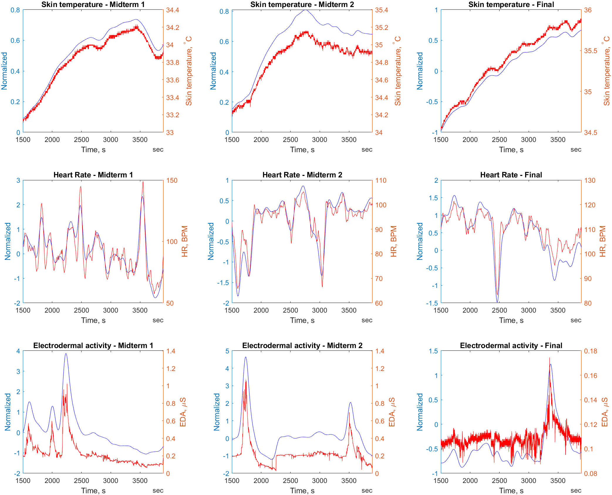
Before further analysis and modeling of the signals was performed, a preprocessing pipeline was implemented to ensure data quality and consistency. First, the signals were truncated to cover only the duration of the exam, ensuring that the analysis focused solely on the relevant data captured during the examination period. Second, linear interpolation has been selected as a method of filling missing data points to maintain the time continuity of the signals and ensure a smooth representation of the data for subsequent analysis. Furthermore, Z-score normalization was used to place the data around the mean and scale based on its standard deviation for the signal, allowing for a consistent comparison and analysis of different signals with different scales and ranges. Lastly, Gaussian smoothing with a three-minute window was specifically selected because it allowed effective removal of high-frequency noise, such as minor fluctuations and artifacts, while preserving important signal features and trends at a meaningful time resolution, ensuring a more accurate representation of the underlying physiological responses for in-depth analysis. The comparison of raw and preprocessed heart rate, EDA and temperature signals in a 40 minute time window is shown in Fig. 1.
Figure 1.
Comparison of preprocessed (blue) and raw (red) signals: temperature, heart rate and electrodermal activity during examination. Each subplot shows a 40-minute window for different examinations, showing the results of preprocessing.
2.3Feature extraction
Using Matlab 2022a, a feature vector comprising 43 different features was extracted from seven signals for the analysis. In total a vector of 301 feature was established:
• Twelve statistical signal features: clearance factor, crest factor, impulse factor, kurtosis, peak value, Signal-to-Noise and Distortion Ratio (SINAD), Signal-to-Noise Ratio (SNR), shape factor, skewness, total harmonic distortion (THD), negative count, positive count;
• Four features obtained from unprocessed signals: mean, root mean square (RMS), standard deviation (Std), median;
• Seven time series features: minimum, median, maximum, first quartile (Q1), third quartile (Q3), autocorrelation function with 1 sample lag (ACF1), partial autocorrelation function with 1 sample lag (PACF1). Note that the median was investigated as a feature of raw and preprocessed signals;
• Twenty spectral features: obtained using the Welch power spectral density estimation method. Features were captured as the amplitude of PSD without its specific frequency.
The set of features comprises fundamental metrics such as mean, median, and standard deviation. Furthermore, the feature collection encompasses characteristics such as the shape factor, the advanced statistics of higher order kurtosis and skewness, along with impulsive metrics related to the peaks of signals, such as clearance factor, crest factor, impulse factor and peak value. The following are the insights into certain features.
1) Clearance factor: an estimate that measures anomalies, or deviations from baseline with a degree of confidence and reliability. It is calculated as the peak value divided by the squared mean value of the square roots of the absolute amplitudes.
2) Crest factor: a parameter used to quantify the ratio of the peak amplitude of a signal to its RMS amplitude. It helps to detect sudden changes or irregularities in physiological signals. A higher crest factor could indicate unexpected events or conditions that require more attention. In contrast, a lower crest factor could represent more stable or consistent physiological patterns. Calculated as a peak value divided by the RMS.
3) Impulse factor: provides information about the intensity or size of a short-term sudden event within a signal. A higher impulse factor often indicates the presence of sudden events within the signal. The mathematical impulse factor is calculated as the ratio of the peak amplitude of the impulse to the average level of the signal.
4) Kurtosis and skewness: high-level statistics provide insight into the system’s behavior by the fourth moment (kurtosis) and the third moment (skewness) of signals. A higher number of outliers in the signal increases the value of the kurtosis metric. Kurtosis has a value of 3 for a normal distribution. Skewness shows asymmetry of the data around the sample mean. The skewness of the normal distribution is zero.
5) Shape factor: quantifies the balance between the positive and negative portions of a signal waveform, providing insights into the overall morphology and balance of the signal. The shape factor relies on the signal’s form, while remaining unrelated to the signal’s dimensions. Calculated by the RMS divided by the mean of the absolute value.
6) Total harmonic distortion: is a parameter used to quantify the level of harmonic components present in a signal relative to their fundamental frequency component. It is used to assess signal quality. A higher THD value could indicate the presence of undesirable harmonics or artifacts that could affect the accuracy and reliability of physiological measurements. THD is calculated as the square root of the sum of the squares of all harmonics divided by the amplitude of the fundamental frequency.
7) Negative and positive counts: shows a number of signal samples below zero or above zero. Essentially, it measures the polarity of a signal. Depending on the type of signal, it can indicate a specific physiological condition (physiological arousal in EDA signals; fever, physical activity, or an increase in metabolic rate in the temperature signal). Mathematically calculated as the number of samples below (or above) zero per second in a signal.
2.4Feature ranking
In this study, the selection of features played an essential role in the transformation of the original set of features, which consisted of 301 candidate features. To investigate the impact of feature selection on the performance and interpretation of the model, feature ranking was used. It allows us to carefully assess the relevance and importance of each feature and to identify those that contributed the most significantly to the predictive power of the model.
Of the 301 features extracted in this study, 299 were found to be consistent with a standard normal distribution. This confirmation was obtained by the use of a Kolmogorov-Smirnov test of one sample, which effectively assessed the compatibility between the distribution of each feature and the normal standard distribution. The high agreement of 299 of the 301 features with the standard normal distribution provides a strong basis for the application of statistical techniques that assume normality and allows for reliable inference and analysis in subsequent modeling and data exploration.
In this research, four feature ranking algorithms were investigated to determine their effectiveness in selecting information features from the dataset. These algorithms include:
• Chi-squared is a statistical method used to select characteristics in categorical data, measuring the dependence between each characteristic and the target variable. It is especially suitable for handling nominal or ordinary variables.
• ReliefF is a popular example-based feature selection algorithm that evaluates the importance of features based on the difference between the features values of a sample and its nearest neighbors. It is commonly used for both regression and classification tasks.
• Variance analysis (ANOVA). Variance analysis is a widely used statistical method to compare the means between several groups of continuous data. Evaluate the importance of each feature in describing the variance in the target variable.
• Kruskal-Wallis is a nonparametric alternative to ANOVA, suitable for continuous data with multiple groups when the normal hypothesis is violated. It ranks features based on differences in their medians in different groups.
The research of these various feature classification algorithms was aimed at identifying the most appropriate techniques to effectively reduce the dimensions and select the most relevant features for subsequent analysis and modeling tasks.
2.5Models for classification
In this research, MATLAB R2022a has been used as a primary tool for studying various models and implementations of popular machine learning algorithms, namely k-Nearest Neighbors (kNN), Random Forests (RF), Multi-Layer Perceptron (MLP), Support Vector Machines (SVM), and Naive Bayes, Discriminant Classifier (DC).
For kNN, parameters such as number of neighbors (k), distance metrics (e.g. Euclidean, Manhattan) and weight functions were varied. In Random Forests, the number of trees in the group, the maximum depth of trees, and the minimum sample per leaf have been changed. In a MLP, the number of hidden layers, the number of neurons in each layer, and the activation functions have been adjusted. In SVM, the kernel functions (e.g. Cubic, Coarse Gaussian), the regularization parameter, and the kernel coefficient were adjusted. In Naive Bayes, assumptions regarding the independence of features and distribution types were tested. For DC, parameters such as regularization strength, kernel, and type of covariation were modified. This extensive parameter adjustment allowed for a thorough study of the sensitivity of each model to different configurations and led to the selection of the most optimal settings for each algorithm in order to achieve higher classification performance.
3.Experiments and results
This chapter presents the experimental results of our research, including experimental setup, classification metrics, and a discussion of the results.
3.1Experiment setup
The model was trained using a 10-fold cross-validation, given the limited size of the data set, which included a total of 30 samples. This approach allows for a stronger assessment of the model performance by iteratively dividing the data into ten subgroups, using nine of them for training and one for validation in each row, thereby mitigating potential overfitting problems and providing a more reliable estimate of its generalization performance.
The marks of the students were transformed into binary values, where a threshold of 80 was applied, with scores above 80 converted to one, representing success, while scores equal to and below 80 were converted to zero, indicating failure.
The scores of all three tests were combined and collectively analyzed, revealing that a total of 12 students achieved points above the 80-point threshold. Among them, three students crossed the threshold for the first half of the semester, four students for the second half of the semester, and five students for the final exam.
3.2Classification metrics
In this investigation, three metrics were used to evaluate the performance of the proposed models in a comprehensive manner: accuracy, area under the Receiver Operating Characteristic Curve (AUROC) and F1-Score. AUROC measured the model’s ability to distinguish between classes with different probability thresholds. The accuracy provided a global perspective on the correctness of the model:
(1)
where
Precision is defined as the ratio of
(2)
Recall or sensitivity is defined as the ratio of
(3)
At the same time, the F1-Score considered the harmonic mean of the precision and recall values, allowing for a balanced assessment of model performance, since the number of classes was slightly unbalanced:
(4)
3.3Results
First, we investigate the feature set without the feature selection algorithm, using the 301 feature. Accuracy score of 0.83, AUROC score of 0.84, and F1-score of 0.78 were achieved (see Fig. 2). This score was obtained using an MLP model with 1 fully connected layer of 25 neurons, ReLU activation function configuration.
Figure 2.
Comparison of feature selection algorithms when selecting a number of features to keep. The x-axis displays the corresponding scores achieved by each algorithm, while the y-axis represents the number of features.
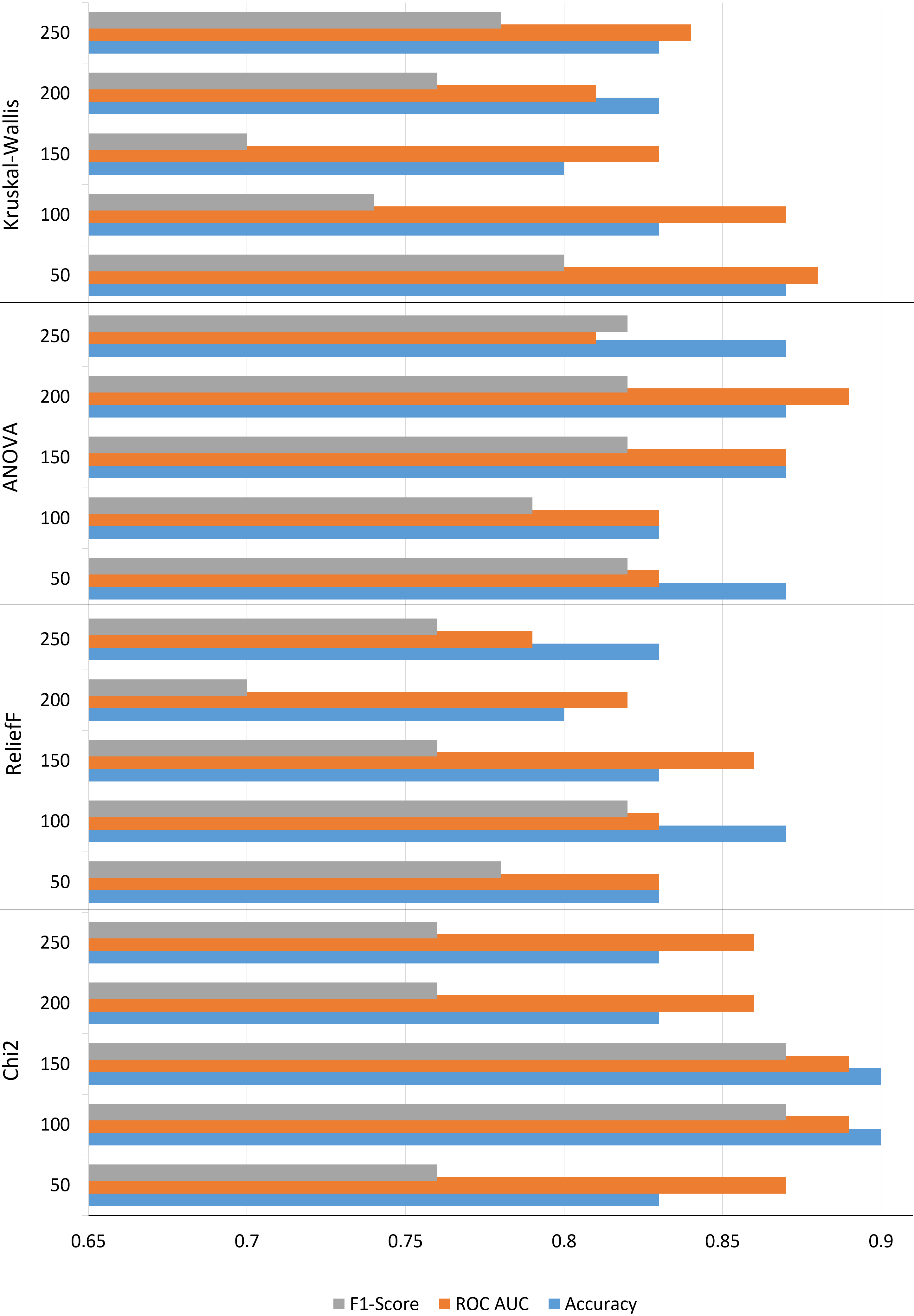
Table 1
Results of Chi2 feature selection algorithm
| Model | Accuracy | AUC | F1-score | Features |
|---|---|---|---|---|
| Quadratic SVM | 0.83 | 0.87 | 0.76 | 50 |
| 2-layer MLP | 0.9 | 0.89 | 0.87 | 100 |
| Linear discriminant | 0.9 | 0.89 | 0.87 | 150 |
| Linear SVM | 0.83 | 0.86 | 0.76 | 200 |
| Linear SVM | 0.83 | 0.86 | 0.76 | 250 |
The highest results of all feature selection algorithms investigated were achieved using the Chi2 feature selection algorithm (Table 1). The table shows the performance of the feature selection algorithm with different numbers of features. In particular, the highest scores were achieved using 100 and 150 features with the corresponding values of accuracy 0.9, AUROC – 0.89 and F1-Score – 0.87. The classification model to achieve the highest score with 100 selected features was a two-layered MLP with two layers with 10 and 50 neurons in the first and second layers, respectively, the ReLU activation function and the standardized data input configuration. Regarding the 150 selected features, the DC classifier achieved the identical score.
Table 2
Results of ReliefF feature selection algorithm
| Model | Accuracy | AUC | F1-score | Features |
|---|---|---|---|---|
| Medium gaussian SVM | 0.83 | 0.83 | 0.78 | 50 |
| Medium gaussian SVM | 0.87 | 0.83 | 0.82 | 100 |
| 1-layer MLP (10 neurons) | 0.83 | 0.86 | 0.76 | 150 |
| Quadratic SVM | 0.8 | 0.82 | 0.7 | 200 |
| 1-layer MLP (100 neurons) | 0.83 | 0.79 | 0.76 | 250 |
Table 3
Results of ANOVA feature selection algorithm
| Model | Accuracy | AUC | F1-score | Features |
|---|---|---|---|---|
| MLP and SVM | 0.87 | 0.83 | 0.82 | 50 |
| Linear SVM | 0.83 | 0.83 | 0.79 | 100 |
| 1-layer MLP (50 neurons) | 0.87 | 0.87 | 0.82 | 150 |
| 2-layer MLP | 0.87 | 0.89 | 0.82 | 200 |
| 1-layer MLP (100 neurons) | 0.87 | 0.81 | 0.82 | 250 |
Table 4
Results of Kruskal-Willis feature selection algorithm
| Model | Accuracy | AUC | F1-score | Features |
|---|---|---|---|---|
| Subspace discriminant | 0.87 | 0.88 | 0.8 | 50 |
| Subspace discriminant | 0.83 | 0.87 | 0.74 | 100 |
| Linear SVM | 0.8 | 0.83 | 0.7 | 150 |
| Linear discriminant | 0.83 | 0.81 | 0.76 | 200 |
| Linear discriminant and MLP | 0.83 | 0.84 | 0.78 | 250 |
Regarding the results of the ReliefF feature selection algorithm (Table 2), the highest score was achieved with 100 selected features with the SVM classifier using a medium Gaussian kernel. The results of the ANOVA feature selection algorithm are presented in Table 3. The highest score was achieved using 200 features. The classification model used in this study was a two-layered MLP with 10 neurons in both layers, the ReLU activation function, and the standardized data input configuration. The results of the Kruskal-Willis feature selection algorithm are presented in Table 4. The highest score was achieved using 50 features. The classification model used in this study was a discriminant model with subspace feature transformation.
Figure 3.
Feature recurrence with investigated feature selection algorithms. The figure presents the recurrence of 43 features, when four different feature selection algorithms were ranked with 100 features. Feature recurrence counted over 7 signals.
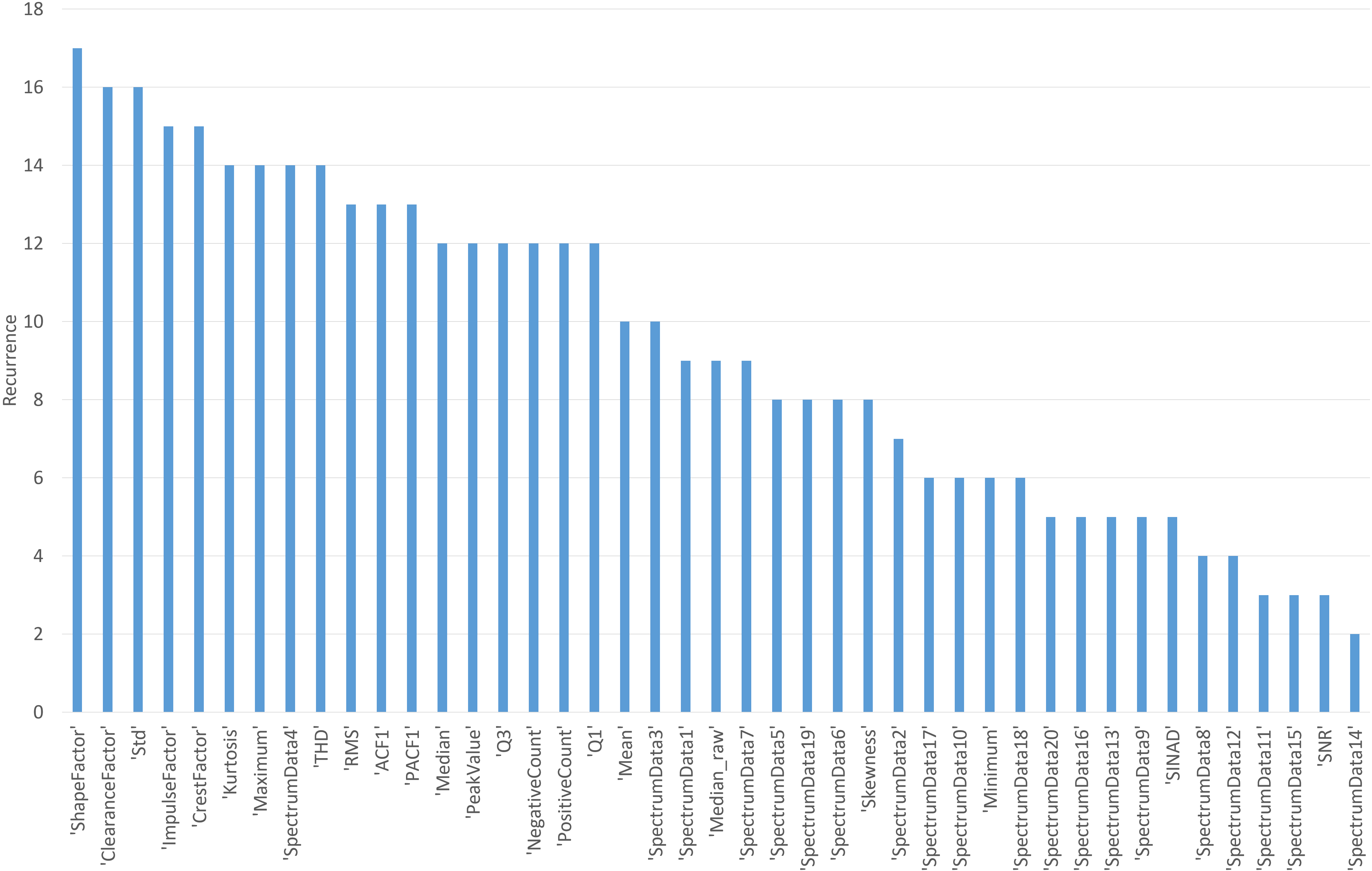
In Fig. 3, we present a feature recurrence plot displaying the selection frequency of 100 ranked features from a pool of 43 features obtained from seven investigated signals. The diagram reflects the general pattern of feature selection across all signals, taking into account the four feature selection algorithms used in the analysis. By visualizing the repetition of these features, the figure shows that shape factor, clearance factor, Std, impulse factor, crest factor, kurtosis, maximum, 4-th spectrum component are prevalent features over all feature selection algorithms. Their recurrence varies from 14 to 17. However, most of the remaining spectrum components (especially above 10), SNR and SINAD are among the most rarely ranked by the feature selection algorithms, with the recurrence between 2 and 5.
Figure 4.
Signal recurrence as feature source with investigated feature selection algorithms. The figure presents the recurrence of source of signal, when four different feature selection algorithms were ranked with 100 features. Signal recurrence counted from 7 signals and 43 features each.
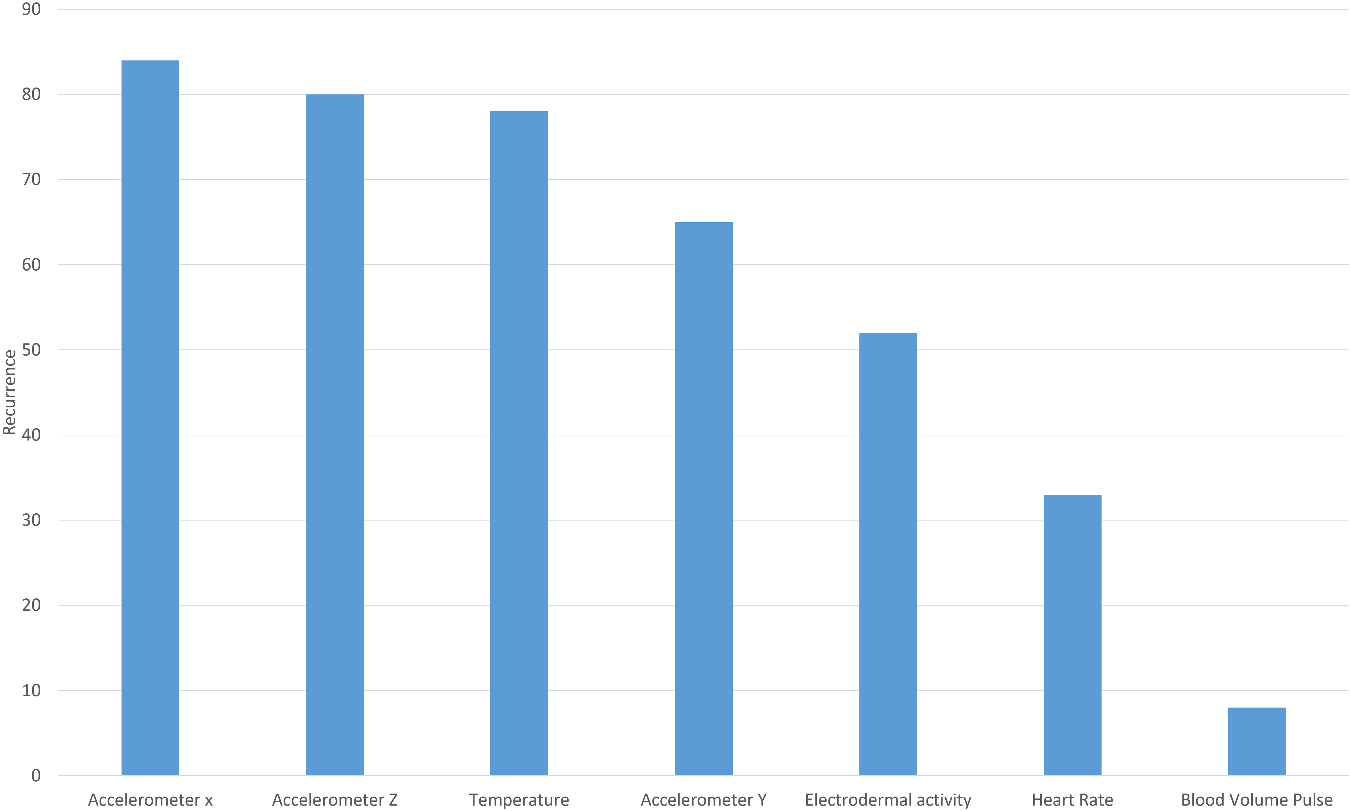
The signal recurrence diagram that represents the signal recurrence as a source of features for the feature selection algorithm is shown in Fig. 4. It can be seen that the accelerometer signals and the temperature signal are most recurrent in contributing features. The heart rate and the PPG signal contribute the lowest number of features, which are ranked high by the feature ranking algorithms.
3.4Discussion and limitations
In this paper, we present our findings on the prediction of grades using physiological signals by investigating various models and feature selection techniques. There are few limitations in the study, namely the relatively small number of subjects. The limited size of the sample may affect the generality of the results, but we believe that the findings of this study offer a guide for future research, especially regarding the types of signals to collect or features to extract. Furthermore, another limitation is the uniform test duration used throughout the study, which cannot fully capture potential performance changes during different exam periods. Future research could examine the impact of different examination phases and perform separate analyzes that include different phases of the exam to further validate and compare the results obtained.
In this study, the performance of various classification algorithms was tested. However, the random tree classifiers did not achieve good results in any of the tests. The data set contained a high number of input features and a small number of output labels. Random tree classifiers tend to overfit in such a data configuration. Despite the mentioned downsides, researchers should not disregard random tree classifiers, especially when working with a larger dataset. With a large amount of data, the risk of overfitting would be mitigated.
Regarding the results in Fig. 3, most of the recurrent features share several common traits. First, they are sensitive to data variation and capable of capturing subtle differences or anomalies in signals. Second, features such as the crest factor or impulse factor may extract meaningful trends, which may correlate with the student score. Finally, recurrent features offer descriptive information on the distribution of the data and may offer some patterns or outliers to explain student scores or exam stress. Alternatively, spectrum components, SNR and SINAD may not inherit most critical features for the prediction of student scores. The features of the spectrum components are more difficult to interpret in the context of student stress or score prediction. SNR and SINAR are used to assess the quality of the signal and do not provide predictive power.
The best results of all the feature selection algorithms examined were obtained using the Chi2 feature selection algorithm. However, in the case of continuous numerical data, feature ranking algorithms such as ANOVA and Kruskal-Wallis are more suitable options compared to Chi-squared (Chi2) and ReliefF, which are usually used for categorical or discrete data. This can be evident when the number of features is reduced to 50. Then ANOVA and Kruskal-Wallis achieved the highest scores between 4 feature ranking algorithms.
The authors of the data set achieved maximum classification accuracy in the range of 0.7 to 0.8 to distinguish between high and low grade predictions using k-Nearest Neighbors classifier [29]. A similar signal classification has been done on this publicly available database in a recent study [30]. The authors focused on skin temperature, heart rate, and EDA signals. The authors investigated various machine learning algorithms; the k-nearest neighbor algorithm showed the highest results of 0.81 AUROC. In a similar investigation, to detect acute mental stress through a 5 min and shorter analysis using 26 features and an empirical mode decomposition classifier. The authors achieved 86.5% (5 min duration) and 90.5% (under 5 min) [26].
The results obtained may have practical applications in education, helping individual students cope with exam stress and improve their academic performance. Future research may focus on personalized stress prediction models and personalized interventions. For educational institutions, the implementation of stress-aware support programs can promote a positive learning environment. However, ethical considerations must be given priority to ensure the privacy of students and their consent to use predictive models. Finding this balance can lead to better student outcomes and enriched educational experiences.
4.Conclusions
A feature vector consisting of 301 distinct features was extracted from seven signals for our investigation. This comprehensive set of features provided valuable information and allowed us to explore the relationships and patterns between signals and student stress during the exam. Investigating the recurrence of features on several sensors and signals further highlights the importance of certain features. Furthermore, the uniform preprocessing technique based on time duration proved effective for all signals, obviating the need for manual filter adjustment.
In addition, this study highlights the effectiveness of various classifiers and feature selection techniques in predicting student exam scores. In particular, DC with linear or subspace feature transformation and MLP emerged as the most promising models, achieving the highest scores on the data set. However, the study also highlights the limitations of certain classifications, such as Random Trees, when dealing with data sets with a large number of input features and a small number of output labels. Furthermore, the analysis of different algorithmic selection features reveals the importance of engineering relevant features for a robust and accurate prediction.
Conflict of interest
None to report.
References
[1] | Chandra Y. Online education during COVID-19: Perception of academic stress and emotional intelligence coping strategies among college students. Asian Education and Development Studies. (2021) ; 10: (2): 229-38. doi: 10.1108/AEDS-05-2020-0097. |
[2] | de la Fuente J, Pachón-Basallo M, Santos FH, Peralta-Sánchez FJ, González-Torres MC, Artuch-Garde R, et al. How has the COVID-19 crisis affected the academic stress of university students? The role of teachers and students. Frontiers in Psychology. (2021) ; 12: : 626340. doi: 10.3389/fpsyg.2021.626340. |
[3] | Khan MJ, Altaf S, Kausar H. Effect of perceived academic stress on students’ performance. FWU Journal of Ocial Sciences. (2013) ; 7: (2). |
[4] | Pascoe MC, Hetrick SE, Parker AG. The impact of stress on students in secondary schooland higher education. International Journal of Adolescence and Youth. (2020) ; 25: (1): 104-12. doi: 10.1080/02673843.2019.1596823. |
[5] | Karaman MA, Lerma E, Vela JC, Watson JC. Predictors of academic stress among college students. Journal of College Counseling. (2019) ; 22: (1): 41-55. doi: 10.1007/s10578-020-00981-y. |
[6] | Helmbrecht B, Ayars C. Predictors of stress in first-generation college students. Journal of Student Affairs Research and Practice. (2021) ; 58: (2): 214-26. doi: 10.1080/19496591.2020.1853552. |
[7] | Crum AJ, Jamieson JP, Akinola M. Optimizing stress: An integrated intervention for regulating stress responses. Emotion. (2020) ; 20: (1): 120. doi: 10.1037/emo0000670. |
[8] | Wilczyńska D, Łysak-Radomska A, Podczarska-Głowacka M, Zajt J, Dornowski M, Skonieczny P. Evaluation of the effectiveness of relaxation in lowering the level of anxiety in young adults – a pilot study. International Journal of Occupational Medicine and Environmental Health. (2019) ; 32: (6): 817-24. doi: 10.13075/ijomeh.1896.01457. |
[9] | Szakonyi B, Vassányi I, Schumacher E, Kósa I. Efficient methods for acute stress detection using heart rate variability data from Ambient Assisted Living sensors. BioMedical Engineering OnLine. (2021) ; 20: (1): 1-19. doi: 10.1186/s12938-021-00911-6. |
[10] | Albaladejo-González M, Ruipérez-Valiente JA, Gomez Mármol F. Evaluating different configurations of machine learning models and their transfer learning capabilities for stress detection using heart rate. Journal of Ambient Intelligence and Humanized Computing. (2022) ; 1-11. doi: 10.1007/s12652-022-04365-z. |
[11] | Elgendi M, Galli V, Ahmadizadeh C, Menon C. Dataset of psychological scales and physiological signals collected for anxiety assessment using a portable device. Data. (2022) ; 7: (9): 132. doi: 10.3390/data7090132. |
[12] | Namvari M, Lipoth J, Knight S, Jamali AA, Hedayati M, Spiteri RJ, et al. Photoplethysmography enabled wearable devices and stress detection: A scoping review. Journal of Personalized Medicine. (2022) ; 12: (11): 1792. doi: 10.3390/jpm12111792. |
[13] | Barki H, Chung WY. Mental Stress Detection Using a Wearable In-Ear Plethysmography. Biosensors. (2023) ; 13: (3): 397. doi: 10.3390/bios13030397. |
[14] | Arsalan A, Majid M, Butt AR, Anwar SM. Classification of perceived mental stress using a commercially available EEG headband. IEEE Journal of Biomedical and Health Informatics. (2019) ; 23: (6): 2257-64. doi: 10.1109/JBHI.2019.2926407. |
[15] | Katmah R, Al-Shargie F, Tariq U, Babiloni F, Al-Mughairbi F, Al-Nashash H. A review on mental stress assessment methods using EEG signals. Sensors. (2021) ; 21: (15): 5043. doi: 10.3390/s21155043. |
[16] | Arsalan A, Majid M. Human stress classification during public speaking using physiological signals. Computers in Biology and Medicine. (2021) ; 133: : 104377. doi: 10.1016/j.compbiomed.2021.104377. |
[17] | Can YS, Arnrich B, Ersoy C. Stress detection in daily life scenarios using smart phones and wearable sensors: A survey. Journal of Biomedical Informatics. (2019) ; 92: : 103139. doi: 10.1016/j.jbi.2019.103139. |
[18] | Zebari R, Abdulazeez A, Zeebaree D, Zebari D, Saeed J. A comprehensive review of dimensionality reduction techniques for feature selection and feature extraction. Journal of Applied Science and Technology Trends. (2020) ; 1: (2): 56-70. doi: 10.38094/jastt1224. |
[19] | Maskeliūnas R, Damaševičius R, Raudonis V, Adomavičienė A, Raistenskis J, Griškevičius J. BiomacEMG: A Pareto-optimized system for assessing and recognizing hand movement to track rehabilitation progress. Applied Sciences. (2023) ; 13: (9): 5744. doi: 10.3390/app13095744. |
[20] | Rajoub B. Characterization of biomedical signals: Feature engineering and extraction. In: Biomedical signal processing and artificial intelligence in healthcare. Elsevier; (2020) ; pp. 29-50. doi: 10.1016/B978-0-12-818946-7.00002-0. |
[21] | Chua KC, Chandran V, Acharya UR, Lim CM. Application of higher order statistics/spectra in biomedical signals – A review. Medical Engineering & Physics. (2010) ; 32: (7): 679-89. doi: 10.1016/j.medengphy.2010.04.009. |
[22] | Wahab MF, Gritti F, O’Haver TC. Discrete Fourier transform techniques for noise reduction and digital enhancement of analytical signals. TrAC Trends in Analytical Chemistry. (2021) ; 143: : 116354. doi: 10.1016/j.trac.2021.116354. |
[23] | Krishnan S, Athavale Y. Trends in biomedical signal feature extraction. Biomedical Signal Processing and Control. (2018) ; 43: : 41-63. doi: 10.1016/j.bspc.2018.02.008. |
[24] | Salankar N, Koundal D, Mian Qaisar S. Stress classification by multimodal physiological signals using variational mode decomposition and machine learning. Journal of Healthcare Engineering. (2021) ; 2021. doi: 10.1155/2021/2146369. |
[25] | Pourmohammadi S, Maleki A. Stress detection using ECG and EMG signals: A comprehensive study. Computer Methods and Programs in Biomedicine. (2020) ; 193: : 105482. doi: 10.1016/j.cmpb.2020.105482. |
[26] | Lee S, Hwang HB, Park S, Kim S, Ha JH, Jang Y, et al. Mental stress assessment using ultra short term HRV analysis based on non-linear method. Biosensors. (2022) ; 12: (7): 465. doi: 10.3390/bios12070465. |
[27] | Pes B. Ensemble feature selection for high-dimensional data: A stability analysis across multiple domains. Neural Computing and Applications. (2020) ; 32: (10): 5951-73. doi: 10.1007/s00521-019-04082-3. |
[28] | Dirgova Luptakova I, Kubovčik M, Pospichal J. Wearable sensor-based human activity recognition with transformer model. Sensors. (2022) ; 22: (5): 1911. doi: 10.3390/s22051911. |
[29] | Amin MR, Wickramasuriya DS, Faghih RT. A Wearable Exam Stress Dataset for Predicting Grades using Physiological Signals. In: 2022 IEEE Healthcare Innovations and Point of Care Technologies (HI-POCT). IEEE; (2022) ; pp. 30-6. doi: 10.1109/HI-POCT54491.2022.9744065. |
[30] | Kang W, Kim S, Yoo E, Kim S. Predicting Students’ Exam Scores Using Physiological Signals. arXiv preprint arXiv: 230112051. (2023) . |


