A submatrix spatial coherence approach to minimum variance beamforming combined with sign coherence factor for coherent plane wave compounding

Yan, Xin; Wang, Yuanyuan

doi:10.3233/THC-228002

A submatrix spatial coherence approach to minimum variance beamforming combined with sign coherence factor for coherent plane wave compounding

Article type: Research Article

Authors: Yan, Xin^a | Wang, Yuanyuan^{a; b; *}

Affiliations: [a] Department of Electronic Engineering, Fudan University, Shanghai, China | [b] Key Laboratory of Medical Imaging Computing and Computer Assisted Intervention of Shanghai, Shanghai, China

Correspondence: [*] Corresponding author: Yuanyuan Wang, Department of Electronic Engineering, Fudan University, Shanghai 200433, China. E-mail: [email protected].

Keywords: Coherent plane wave compounding, spatial coherence, minimum variance, ultrasound imaging, sign coherence factor

DOI: 10.3233/THC-228002

Journal: Technology and Health Care, vol. 30, no. S1, pp. 11-25, 2022

Published: 25 February 2022

Get PDF

Abstract

BACKGROUND:

The coherent plane wave compounding (CPWC) is a promising technique to enhance the imaging quality while maintaining the high frame rate in the plane wave ultrasound imaging. Recently, the spatial-coherence-based method has been specially designed to process echo matrix required by the minimum variance (MV) method.

OBJECTIVE:

In this paper, a novel beamforming method that integrates the submatrix-spatial-coherence-based MV with the sign coherence factor (SCF) is proposed to further improve the imaging quality.

METHOD:

The submatrix smoothing technique is modified to smooth and de-correlate signals of the receiving array dimension. Then, the SCF is used to modify the input vector of the beamformer, which can reduce side lobe noises with almost no increase in the amount of calculation. Simulation, phantom, in vivo, and sound velocity error experiments have been performed to verify the superiority of the proposed beamformer.

RESULTS:

The imaging results show that the proposed approach performs better in the imaging resolution and contrast compared to the traditional CPWC method.

CONCLUSION:

The robustness of the proposed method is enhanced, and the over-suppression phenomenon can be alleviated, which is a phenomenon that occurs in the original spatial-coherence and SCF methods.

1.Introduction

The plane wave imaging (PWI) is an effective mode to realize ultrafast ultrasound imaging for the visualization of rapid tissue motions [1, 2]. However, it causes the significant reduction in the imaging quality due to emitting unfocused plane waves. Lu and Cheng proposed the plane wave compounding (PWC) method to provide enhancement of the imaging quality without affecting the frame rate in the plane wave modality [3, 4, 5]. Montaldo et al. modified the PWC in 2009 and named it as the coherent plane wave compounding (CPWC). Here the echo signals from different firing angles were compounded to improve the image quality [6, 7].

The adaptive beamforming algorithm dynamically calculates the weight vector of received echo signals. Compared to the conventional delay and sum (DAS) algorithm, it can effectively enhance the ultrasound imaging quality [8]. In 1969, Capon proposed the minimum variance (MV) algorithm, which was one of representative adaptive beamforming algorithms. The core of the method is calculating the undistorted weighting vector by minimizing the output energy of the beamformer dynamically [9, 10]. The method improves the imaging resolution and suppresses the interference noise significantly.

The coherence factor (CF) is another typical adaptive beamformer. It calculates the ratio of the coherent energy to the total energy of echo signals and works as a multiplier to constrain the output of the beamformer. The phase coherence factor (PCF) is also a coherence-based method. It uses the signal phase dispersion to design the factor, which is different from the CF. The sign coherence factor (SCF) is a special case of the PCF [11]. It is simple to calculate and easy to implement. All coherence-based methods can reduce sidelobes and improve the imaging contrast. However, these methods will reduce the brightness of the speckle region owing to the over-suppression of desired signals. In addition, MV-based, CF-based and MV-CF combined methods have been extensively applied to the CPWC imaging mode [12, 13, 14].

Recently, several methods based on the MV and CF have been modified for the 2-D echo dataset of the CPWC. The joint MVDR (JTR) method proposed by our group computes two MV weighting vectors: the transmitting aperture weighting vector and receiving aperture weighting vector [15, 16]. By combining two vectors, the beamformer can obtain a significant improvement in the imaging resolution. Data compounded among transmit (DCT) MV and data compounded among receive (DCR) MV beamformers were both proposed by Nguyen et al., who used different combinations of signals to estimate the covariance matrix. It is covenient to implement since the MV weight only needs to be calculated once [17]. These two beamformers are based on the van Cittert-Zernike theorem and can improve the imaging resolution and contrast [18, 19]. However, the diagonal loding factors used by these two beamformers are much larger than the conventional range, which is the limitation of two beamformers. In addition, the over-suppression phenomenon will occur in the DCT-MV method with a small loading factor, which may affect the contrast ratio (CR) and contrast-to-noise ratio (CNR) values.

In this paper, a submatrix-spatial-coherence combined with SCF method is proposed to implement the MV beamforming, which can enhance the imaging quality of the CPWC. We use submatrix smoothing technique to divide the data matrix into overlapped submatrices over the receive dimension and full data is preserved along the transmit dimension. Afterwards, the submatrix spatial coherence is estimated to approximate the sub-covariance matrix. After averaging all results of submatrices, the final covariance matrix can be obtained. The input data vector of the beamformer is obtained by compounding data over multiple transmits of the average submatrix, which is also corrected by the SCF. There are three advantages of the method. First, the proposed beamformer achieves the better performance both on the resolution and contrast compaired with the CPWC. Second, the speckle region is preserved well. Third, the robustness is significantly improved.

The contents of other chapters are arranged as follows. The theories of existing approaches are illustrated in Section 2. The novel beamformer is described in detail in Section 3. In Section 4, the set up and results of the simulation, phantom, in vivo and sound velocity error experiments are described. In Sections 5 and 6, the discussion and conclusion are given respectively.

2.Background

2.1Coherent plane wave compounding

For the CPWC imaging mode, we record the echo signals into a two-dimensional matrix for beamforming [6]. Here we assume that the number of transducer elements is M and the number of steering beams is N, and the data matrix 𝐗⁢(n) can be denoted by:

(1)

𝐗⁢(n)=[x1,1⁢(n)x1,2⁢(n)⋯x1,M⁢(n)x2,1⁢(n)x2,2⁢(n)⋯x2,M⁢(n)⋮⋮⋱⋮xN,1⁢(n)xN,2⁢(n)⋯xN,M⁢(n)]

where xi,j⁢(n) is the ith transmission beam signal received by the jth array element, and n represents the time index. By superimposing and averaging all received signals in 𝐗⁢(n), the beamforming output is expressed as follows:

(2)

y𝐶𝑃𝑊𝐶⁢(n)=1M⁢N⁢∑i=1NωT⁢(i)⁢∑j=1MωR⁢(j)⁢xi,j⁢(n)

where ωR and ωT are weights of the receiving and transmitting apodization respectively.

2.2Minimum variance beamformer

The mathematical expression of MV is as follows:

(3)

y⁢(n)=𝐰H⁢(n)⁢𝐱⁢(n)=∑k=1MwkH⁢(n)⁢xk⁢(n)

where (⋅)H represents the matrix conjugate transpose, w⁢(n) is the MV weighting vector and 𝐱⁢(n) is the received echo signals after time delays.

The MV method calculates the undistorted weighting vector by a constraint process that minimizes the output power of the beamformer. It can be expressed as:

(4)

min𝐰𝐰H⁢𝐑⁢(n)⁢𝐰,subject to 𝐰H⁢𝐚=𝟏

where 𝐑⁢(n) represents the covariance matrix, a represents the steering vector, which is an all one vector.

The solution of the above equation can be computed through the Lagrange multiplier approach:

(5)

𝐰M⁢V=𝐑-1⁢𝐚 aH⁢𝐑-1⁢𝐚.

𝐑⁢(n) is usually approximated to the sample covariance matrix:

(6)

𝐑^⁢(n)=E⁢[𝐱⁢(n)⁢ xH⁢(n)].

The estimation of 𝐑^⁢(n) is a key part of the MV algorithm, so that the spatial smoothing process is used to improve its accuracy. By dividing the receiving array into multiple overlapping subarrays, the sub-covariance matrix can be calculated in each subarray. By averaging each result, the final 𝐑^⁢(n) is obtained:

(7)

𝐑^⁢(n)=1M-L+1⁢∑l=1M-L+1𝐱l⁢(n)⁢𝐱lM⁢(n)

where 𝐱l⁢(n) is the lth subarray and L is the subarray length.

Diagonal loading technique is also applied to the covariance matrix to obtain a comparably stable matrix. We use 𝐑^⁢(n)+ε×𝐈 to replace 𝐑^⁢(n), where ε represents the diagonal loading factor. It is usually expressed as Δ×(𝑡𝑟𝑎𝑐𝑒⁢[𝐑^⁢(n)]/L), where Δ is usually between 0.01 ∼ 0.2, and I is the identity matrix.

The output of the MV beamformer is as follows:

(8)

yM⁢V⁢(n)=1M-L+1⁢∑l=1M-L+1 wM⁢VH⁢(n)⁢𝐱l⁢(n).

2.3Sign coherence factor beamformer

To implement SCF, the normalized phase space [-π,π] is divided into two sub-intervals (-π/2,π/2] and [-π,-π/2]∪(π/2,π]. If the phases of the aperture data all fall into the same interval, the data can be considered completely coherent with the same polarity. Therefore, the SCF designs the factor by using the sign bit instead of the phase of the data. The sign bit b⁢(n) of the data no less than zero is set to +1, otherwise b⁢(n) is set to -1. The variance of b⁢(n) can be expressed as:

(9)

σ2=1-(1M⁢∑i=1Mbi⁢(n))2.

σ2 ranges from 0 to 1, and the SCF is defined as:

(10)

𝑆𝐶𝐹p⁢(n)=|1-σ|p.

where p is the factor used to regulate the effect of the SCF method.

2.4Data compounded among transmit MV beamformer

This method estimates the covariance matrix by using different combinations of echo signals for each transmission angle [17]. For the 2-D data matrix 𝐗⁢(n), DCT-MV uses a data vector 𝐯⁢(n)=[v1⁢(n),v2⁢(n),…⁢vM⁢(n)]T as the input vector of the beamformer, where

(11)

vj⁢(n)=∑i=1Nxi,j⁢(n)⁢ for ⁢j=1→M

vj⁢(n) is the accumulated signal over all transmit beams on the jth element, N is the number of steered transmitting beams and M is the element number.

Then the covariance matrix of 𝐯⁢(n) is approximated to the second-order statistics of several new snapshots of the data pk⁢(n)=[pk,1⁢(n),pk,2⁢(n),…,pk,M⁢(n)]T, where

(12)

pk,j⁢(n)=1N-1⁢∑i=1i≠kNxi,j⁢(n)

For every transmit event, 𝐩k⁢(n) can be generated to calculate the covariance matrix (k=1→N). By averaging these results, the final covariance matrix of the DCT-MV can be obtained:

(13)

𝐑^𝐷𝐶𝑇=1N⁢∑k=1N𝐩k⁢(n)⁢𝐩kH⁢(n)+ε⁢ I

where ε represents the diagonal loading factor, I represents the identity matrix. The schematic of DCT-MV beamformer is described in Fig. 1a.

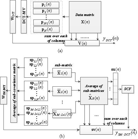
Figure 1.

Schematics of two beamformers: (a) DCT-MV, (b) SM-DCT MV.

3.Methods

The proposed method is the sub-matrix data compounded among transmit MV beamformer combined with the SCF. It is named as SM-DCT MV for short. We build a new data matrix by dividing the original 2-D data matrix into overlapping submatrices. Different to the submatrix technique used by Qi et al. [16], we just smooth the data on the receive dimension and full data are kept on the other transmit dimension. It is described as follows:

(14)

𝐗^=[𝐗¯1,𝐗¯2,…,𝐗¯M-L+1]

𝐑^ can be considered as a N×L×(M-L+1) size 3-D data matrix, L is the subarray length and the lth submatrix 𝐗¯l is expressed as follows:

(15)

𝐗¯l=[xl1xl+11⋯xl+L-11xl2xl+12⋯xl+L-12⋮⋮⋱⋮xlNxl+1N⋯xl+L-1N]

We take the average of these overlapping submatrices X¯l as the input matrix 𝐗^R (a N×L size 2-D data matrix). It can be viewed as the data matrix of original signals after the decorrelation processing across the receiving aperture dimension.

(16)

𝐗^R=1M-L+1⁢∑l=1M-L+1𝐗¯l

The input vector of the proposed SM-DCT beamformer can be obtained by a data vector compounded over different transmits afterwards. Considering that multiple steering angle signals have a certain coherence to the imaging result of the same imaging target, and the coherence to the noise and clutter is poor. Therefore, the SCF factor is used as a correction to obtain a more accurate input signal vector. First, a vector is obtained by compounding the columns of 𝐗^R, which represents imaging results of different beams at the same point. Second, the SCF can be calculated (described in Section 2.3) [20]. We denote the final input vector by 𝐬𝐯⁢(n)=𝑠𝑐𝑓p*[s⁢v1⁢(n),s⁢v2,…⁢s⁢vL⁢(n)], where

(17)

s⁢vj⁢(n)=∑i=1Nxi,j⁢(n)⁢ for ⁢j=1→L

where i and j are reused in 𝐗^R, representing the transmit event and submatrix receive element index.

Then, the new set of snapshot 𝐬𝐩k⁢(n)=[s⁢pk,1⁢(n),s⁢pk,2⁢(n),…,s⁢pk,L⁢(n)]T can be generated, where

(18)

s⁢pk,j⁢(n)=1N-1⁢∑i=1i≠kNxi,j⁢(n)

Afterwards, N vectors of 𝐬𝐩k⁢(n) can be obtained by over all firing angles. The sub-covariance matrix can be obtained:

(19)

𝐗^l=1N⁢∑k=1N𝐬𝐩k⁢(n)⁢𝐬𝐩kH⁢(n)

By averaging all results, the covariance matrix similar to the second-order statistics of 𝐬𝐯⁢(n) is obtained. We denote it as

(20)

𝐗^SM-DCT=1M-L+1⁢∑l=1M-L+1𝐗^l+ε⁢𝐈

where ε represents the diagonal loading factor, I is the identity matrix.

It is worth mentioning that we can obtain the 𝐬𝐩k⁢(n) by compounding different combinations of data first and smoothing it later. Compared with the method of smoothing first and recombination later, it saves a cycle of calculating time, but the result is consistent. The schematic of SM-DCT beamformer is shown in Fig. 1b.

4.Experiments and results

4.1Experiment setup

The performance of different beamformers was evaluated using the CPWC through simulation, phantom, in vivo and sound velocity error experiments. The simulation data was acquired using Field II, the phantom and in vivo data was obtained using Verasonics ultrasound platform. The processing of different algorithms are implemented on the MATLAB platform.

For all simulations, a 128-element transducer with 0.3 mm pitch, centered at 5 MHz, was used to acquire simulation data. Both transmitting and receiving processes used full array elements. The sampling rate was 40 MHz. We simulated four point targets placed at z= (30, 40, 50, 60 mm) for the resolution evaluation, and a cyst target with 2.5 mm radius located at (x,y,z)= (0, 0, 50 mm) was used to assess the imaging contrast. For the phantom experiments, the transducer array configuration we used is the same as the simulation experiment. For in vivo data, we collected the carotid artery data from a healthy adult male. The sound velocity error experiment was performed to study the robustness of algorithms. The sound velocity value was set to 1540 m/s, and then changed by 2%, 5% for the point imaging. The point was set at z= 40 mm. To implement the plane wave imaging, 49 plane waves were emitted in the range of -12∘ to 12∘ degrees, which were 0.5∘ degrees apart from each other.

4.2Parameters and evaluation metrics

Parameters selected in the experimental evaluation are explained here. For the proposed SM-DCT beamformer, the submatrix length L is set to 0.4 times the receiving array length for the point imaging and 0.3 times the receiving array length for the cysts imaging, respectively. Δ in the diagonal loading is set to 0.01. In all experiments, we select different values of parameter p used by the SCF to evaluate the imaging results. For the DCT beamformer, Δ in the diagonal loading is set to 1 for the point target simulation and 5 for other experiments. F-number is set to 1.

Evaluation metrics are used for the quantitative measurement. The full width of mainlobe (FWHM) is used to evaluate the imaging resolution, and it is usually estimated by the mainlobe width at -6 dB and -20 dB. For the measurement of the contrast, the CR, CNR and the speckle-signal-to-noise ratio (s-SNR) are adopted in the cyst target study. They are defined as follows:

(21)

CR=20⁢log10⁡(μi⁢/⁢μo),

(22)

CNR=|μ-iμo|σi2+σo2,

(23)

s-SNR=μiμo

where μi and μo represent the average amplitude of signals inside and outside the cyst. σi and σo are standard deviations of μi and μo respectively.

4.3Simulated study

Point target simulation results of different beamforming algorithms are presented in Fig. 2.

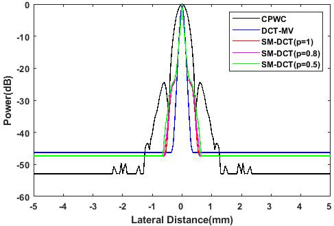
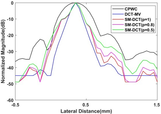
Figure 2a shows the imaging result of traditional CPWC method. It can be seen that the main lobe is wide and side lobes are obvious. In Fig. 2b, the DCT-MV method achieves a narrow mainlobe and no visible sidelobes. Figure 2c–e are results of the SM-DCT MV with p= 1, 0.8 and 0.5. It can be seen that the width of the mainlobe and the amplitude of sidelobes are all performed better than those of the CPWC.

In order to evaluate the imaging resolution quantitatively, the transverse beam amplitude response diagram at z= 50 mm is given in Fig. 3, and FWHM values at -6 dB and -20 dB of different beamformers are shown in Table 1. It shows that the -6 dB mainlobe width of the SM-DCT MV is 0.13 mm, which is slightly lower than that of the DCT-MV (0.17 mm). While the -20 dB mainlobe width of the SM-DCT MV (0.38 mm) is slightly higher than that of the DCT-MV (0.34 mm). Nevertheless, metrics of the proposed method are all better than those of the CPWC. Different values of the parameter p used by the SCF have different effects on the sidelobe suppression. The larger p is, the better effect achieves.

Table 1

FWHM at -6 dB and -20 dB for simulated point targets at the depth of z= 50 mm

Beamformer	FWHM (mm)
CPWC	0.49/0.80
DCT-MV	0.17/0.34
SM-DCT (p= 1)	0.13/0.38
SM-DCT (p= 0.8)	0.13/0.38
SM-DCT (p= 0.5)	0.13/0.38

Figure 2.

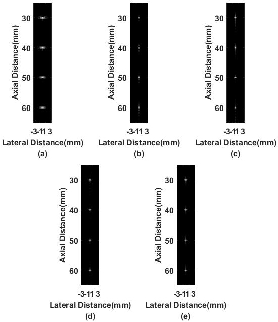
Simulated point targets imaging results: (a) CPWC, (b) DCT-MV, (c) SM-DCT MV (p= 1), (d) SM-DCT MV (p= 0.8), (e) SM-DCT MV (p= 0.5). All results in the figure are displayed within a -60 dB dynamic range.

Figure 3.

The transverse beam amplitude response diagram at the depth of z= 50 mm.

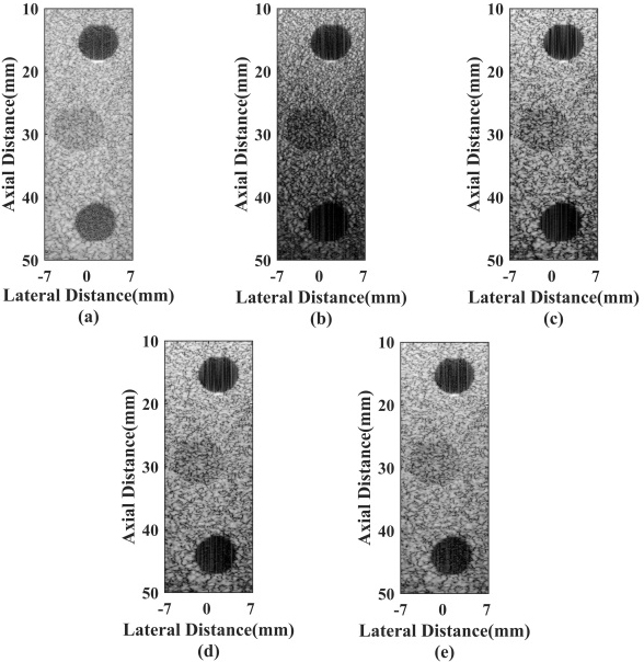
Cyst simulation results of different beamformers are given in Fig. 4. Figure 4a shows the imaging result of the CPWC. The noise level inside the cyst is high, which is caused by the high sidelobe amplitude of the traditional method. The result of the DCT-MV shows that the internal imaging achieves the better noise suppression, and the edge of the cyst is clear. However, the brightness of the speckle region is weakened, which results in the unsatisfactory contrast. As seen from Fig. 4c–e, results of the SM-DCT MV with p= 0.8, 0.5 and 0.3 have the better performance in the speckle region compared with Fig. 4b.

Table 2

CR, CNR and s-SNR for simulated cysts

Beamformer	CR (dB)	CNR	s-SNR
CPWC	33.91	1.69	1.51
DCT-MV	30.41	0.76	1.15
SM-DCT (p= 0.8)	36.63	1.30	1.32
SM-DCT (p= 0.5)	37.30	1.39	1.34
SM-DCT (p= 0.3)	37.00	1.48	1.39

The values of CR, CNR and s-SNR are displayed in Table 2 for quantitative assessment. It can be seen that the contrast of the SM-DCT with p= 0.5 is the highest one, which is 10% and 22.7% higher than that of CPWC and DCT-MV, respectively. The CNR value of the SM-DCT MV with p= 0.5 achieves an improvement of 0.63 compared with the DCT-MV. The s-SNR values of the proposed method are also slightly improved compared with that of the DCT-MV. These numerical enhancements prove that the SM-DCT MV can improve the imaging contrast while maintaining a good speckle background region.

4.4Experimental phantom study

Figure 5 gives imaging results of the point targets phantom. It can be noted that although the DCT-MV method has a better point imaging effect, its speckle background is over-suppressed, leading to the loss of the image information. While the proposed SM-DCT method avoids this phenomenon successfully, the brightness of the speckle region keeps well.

Table 3

FWHM at -6 dB and -20 dB for point phantom at the depth of z= 30 mm

Beamformer	FWHM (mm)
CPWC	0.42/0.66
DCT-MV	0.15/0.38
SM-DCT (p= 1)	0.17/0.51
SM-DCT (p= 0.8)	0.17/0.54
SM-DCT (p= 0.5)	0.17/0.59

Figure 4.

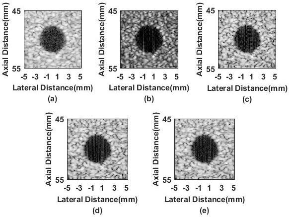
Simulated cysts imaging results: (a) CPWC, (b) DCT-MV, (c) SM-DCT (p= 0.8), (d) SM-DCT (p= 0.5), (e) SM-DCT (p= 0.3). All results in the figure are displayed within a -60 dB dynamic range.

Figure 5.

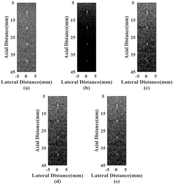
Experimental point targets phantom imaging results: (a) CPWC, (b) DCT-MV, (c) SM-DCT (p= 1), (d) SM-DCT (p= 0.8), (e) SM-DCT (p= 0.5). All results in the figure are displayed within a -60 dB dynamic range.

Figure 6.

Transverse beam amplitude response diagrams at the depth of z= 30 mm.

The transverse beam amplitude response diagrams at z= 30 mm is shown in Fig. 6. Table 3 lists FWHM values (-6 dB and -20 dB) for the statistical evaluation. Values show that the SM-DCT’s -6 dB mainlobe width is slightly higher than that of the DCT-MV. Nevertheless, it is still narrower than that of the CPWC. The SCF with p= 0.8 achieves a narrower mainlobe width at -20 dB than the SCF with p= 0.5 and p= 0.3.

Results of the cysts phantom are presented in Fig. 7. Figure 7a shows that the noise level inside the cysts is obvious with the CPWC. Figure 7b is the result of the DCT-MV beamformer. The internal imaging of cysts is good, while the speckle area is weakened. From Fig. 7c–e, the proposed SM-DCT beamformer performs better in the internal imaging than the CPWC and the speckle background preserved better than the DCT-MV.

Table 4

CR, CNR, ands-SNR for experimental cysts

Beamformer	CR (dB)	CNR	s-SNR
CPWC	28.35/16.02	1.91/1.61	1.99/1.93
DCT-MV	28.63/13.01	1.17/0.89	1.21/1.16
SM-DCT (p= 0.8)	33.51/19.59	1.43/0.89	1.46/1.00
SM-DCT (p= 0.5)	33.72/20.46	1.53/1.08	1.57/1.19
SM-DCT (p= 0.3)	33.25/19.84	1.63/1.25	1.67/1.39

Figure 7.

Experimental cysts phantom imaging results: (a) CPWC, (b) DCT-MV, (c) SM-DCT (p= 0.8), (d) SM-DCT (p= 0.5), (e) SM-DCT (p= 0.3). All results in the figure are displayed within a -60 dB dynamic range.

CR, CNR, and s-SNR values are given in Table 4 for quantitative assessment. For the cyst at z= 15 mm, the CR of the SM-DCT (p= 0.5) is 17.8% and 18.9% higher than that of the DCT-MV and CPWC. For the cyst at z= 45 mm, the CR of the SM-DCT (p= 0.5) is 57.3% and 27.7% higher than that of the DCT-MV and CPWC. The SM-DCT also achieves the improvement in CNR and s-SNR values compared with DCT-MV.

4.5In vivo study

Figure 8 shows results of different beamformers using carotid artery data from an adult male. The result is similar to the cyst phantom experiment because of the similarity between the circular artery and the anechoic cyst. From Fig. 8a, it can be seen that noises are obvious inside the vessel with the CPWC. Other beamformers achieve the better performance on reducing the noise level. The proposed SM-DCT beamformer distinguishes the arteries and boundaries well, and the surrounding information preserved more completely.

Table 5

CR, CNR, and s-SNR for in vivo carotid artery

Beamformer	CR (dB)	CNR	s-SNR
CPWC	21.87	1.14	1.25
DCT-MV	19.12	0.67	0.77
SM-DCT (p= 0.8)	27.45	0.55	0.58
SM-DCT (p= 0.5)	27.97	0.71	0.74
SM-DCT (p= 0.3)	25.90	0.86	0.90

Figure 8.

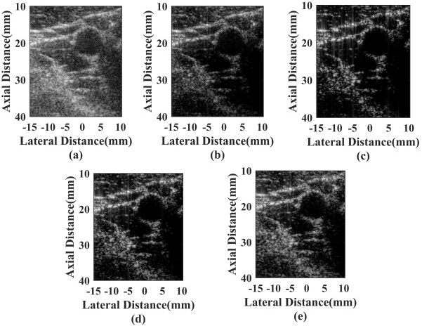
In vivo human carotid artery imaging results: (a) CPWC, (b) DCT-MV, (c) SM-DCT (p= 0.8), (d) SM-DCT (p= 0.5), (e) SM-DCT (p= 0.3). All results in the figure are displayed within a -60 dB dynamic range.

The internal and external signals of the carotid artery are used to calculate the CR, CNR, and s-SNR values. Results are presented in Table 5 for the statistical assessment. Similar to the cyst phantom experiment, the CR of the SM-DCT (p= 0.5) increases 46.3% and 27.9% compared to that of the DCT-MV and CPWC respectively. Also, the CNR and s-SNR are both higher than those of the DCT-MV.

Figure 9.

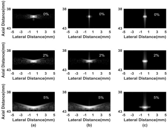
Simulated point imaging results of different sound velocity errors: (a) CPWC, (b) DCT-MV (Δ= 5), (c) SM-DCT (Δ= 0.01, p= 1). All results in the figure are displayed within a -60 dB dynamic range.

4.6Robustness to sound velocity error

Point imaging results for different sound velocity errors with different beamformers are given in Fig. 9. In Fig. 9a and b, the mainlobe width of the CPWC and DCT-MV widened and the sidelobes increased obviously with the increase of the sound velocity error. Figure 9c shows that the sidelobe level of the proposed method is lower compared with the former two methods. Point imaging results of the SM-DCT are less affected by the sound velocity and the robustness is better.

5.Discussion

From results, the SM-DCT method proposed in this paper shows its advantages in the plane wave compounding mode in terms of the enhancement of the imaging quality and the improvement of algorithm robustness. These performance advantages mainly result from two aspects. First, a submatrix spatial smoothing technique is added to the spatial coherence method to fully de-correlate received signals. By this way, a more accurate covariance matrix can be obtained, and the non-singularity of the covariance matrix can be guaranteed. In addition, the diagonal loading factor chosen in the SM-DCT MV can be a typical value. Both of the spatial smoothing and low loading factor lead to the improvement of the robustness of the algorithm. Second, the SCF is used to correct the input vector of the beamformer, which improves the imaging contrast while maintaining the mainlobe width at -6 dB, as shown in Fig. 3. Since the SCF is calculated by the smoothed submatrix, the over-suppression problem of signals in the speckle region has been avoided, as shown in Figs 4, 5, 7 and 8. In addition, the SCF contributes to the robustness of the algorithm. All imaging results prove the superiority of the proposed algorithm.

As for several parameters used in all experiments, the selection of the length of submatrix L and the diagonal loading factor affects the imaging result. A higher L means that a larger number of effective elements are used, which can achieve the better imaging resolution, while the contrast slightly reduced, and vice versa. Different diagonal loading factors also achieve different imaging results. It can be regarded as a very small white noise added to diagonal elements of the covariance matrix. This disturbance should not be too large, a small value can also ensure the robustness of the algorithm [8]. However, the original DCT method has the limitation of choosing a much higher factor, as illustrated in literature [17]. From Figs 4b and 5b, it can be noted that the DCT method occurs over-suppression phenomenon in speckle background with Δ= 5, which results in the unsatisfactory contrast. It is precisely because the value of Δ is not large enough. To explore this phenomenon, we have added additional experiments. If Δ is increased to 30, the phenomenon can be improved, and the CR value can be better than CPWC. However, the diagonal loading factor is too large, and the mainlobe width is widened at the same time. In the proposed method, there is no need to constantly adjust the diagonal loading factor. Therefore, it alleviates the over-suppression phenomenon with Δ= 0.01 (the normal condition) owing to the smoothing process and obtains the improvement of imaging contrast resulting from the using of the SCF.

In addition to the above advantages, the proposed method also has certain limitations. From Figs 3 and 6, the mainlobe width at -20 dB is wider compared with DCT-MV and needs to be further improved. Anyway, it is better than CPWC. Also, the calculation complexity of the SM-DCT is slightly increased compared with the DCT-MV. It is summarized in detail. For the CPWC with N firing events, it calculates MV weights and SCF for only once. The calculation of the SCF can be negligible because the process is extremely simple. For the SM-DCT beamformer, the number of operations required to obtain the MV weight is approximately 2⁢L3/3+L2+L+L+N×L2×(M-L+1). While the computational amount of the DCT-MV is approximately 2⁢M3/3+M2+M+M+N×M2. Although the proposed method reduces the calculation amount of the covariance matrix inverse owing to the reduction of the matrix dimension, the process of obtaining the covariance matrix is improved by M-L+1 computes in each submatrix. Generally speaking, the amount of calculation of SM-DCT MV is higher than that of the DCT-MV. However, the computation amount of the SM-DCT still has advantages compared to other methods using the spatial smoothing technique owing to the only once calculation of MV weights. The execution times of the DCT-MV and SM-DCT MV are measured using MATLAB on PC (Windows 10, 64-bit system, Intel Xeon CPU E5-2687W v4, and 64-Gb memory). The results are about (630 ± 5s) and (780 ± 5s) for the DCT-MV and SM-DCT MV respectively.

6.Conclusion

A novel beamformer based on the spatial coherence method integrating the submatrix smoothing technique and sign coherence factor is proposed. Simulated and experimental results show that the SM-DCT MV obtained higher CR, CNR and s-SNR values compared with the DCT-MV method under a small diagonal loading factor condition. The -20 dB mainlobe width of the SM-DCT is wider than that of the DCT-MV, while -6dB perform well. Both of them are better than the CPWC. More importantly, the sound velocity error experiment proves that the robustness of the SM-DCT method is improved in terms of the sidelobe reduction. Furthermore, the over-suppression phenomenon of the speckle region is alleviated. In consideration of above performances, we consider that the proposed beamformer achieves the improvement on the imaging quality and robustness in the CPWC imaging modality.

Acknowledgments

This work is supported by the National Natural Science Foundation of China (61771143 and 81627804).

Conflict of interest

None to report.

References

[1]	Wells, and PNT. Ultrasound imaging. Physics in Medicine & Biology. (2006) ; 51: (13): 83–98. doi: 10.1074/jbc.273.41.26317.
[2]	Tanter M, Fink M. Ultrafast imaging in biomedical ultrasound. IEEE Transactions on Ultrasonics, Ferroelectrics and Frequency Control. (2014) ; 61: (1): 102–119. doi: 10.1109/TUFFC.2014.2882.
[3]	Berson M, Roncin A, Pourcelot L. Compound scanning with an electrically steered beam. Ultrasonic Imaging. (1981) ; 3: (3): 303–308. doi: 10.1016/0161-7346(81)90162-0.
[4]	Lu JY. Experimental study of high frame rate imaging with limited diffraction beams. IEEE Transactions on Ultrasonics, Ferroelectrics, and Frequency Control. (1998) ; 45: (1): 84–97. doi: 10.1109/58.646914.
[5]	Cheng JQ, Lu JY. Extended high-frame rate imaging method with limited-diffraction beams. IEEE Transactions on Ultrasonics, Ferroelectrics, and Frequency Control. (2016) ; 53: (5): 880–899. doi: 10.1109/TUFFC.2006.1632680.
[6]	Montaldo G, Tanter M, Bercoff J, Benech N, Fink M. Coherent plane-wave compounding for very high frame rate ultrasonography and transient elastography. IEEE Transactions on Ultrasonics, Ferroelectrics and Frequency Control. (2009) ; 56: (3): 489–506. doi: 10.1109/TUFFC.2009.1067.
[7]	Austeng A, Nilsen CIC, Jensen AC, Nasholm SP, Holm S. Coherent plane-wave compounding and minimum variance beamforming. Proceedings of the IEEE Ultrasonics Symposium. (2011) ; 2448–2451. doi: 10.1109/ULTSYM.2011.0608.
[8]	Synnevag JF, Austeng A, Holm S. Adaptive beamforming applied to medical ultrasound imaging. IEEE Transactions on Ultrasonics, Ferroelectrics and Frequency Control. (2007) ; 54: (8): 1606–1613. doi: 10.1109/TUFFC.2007.431.
[9]	Capon J. High-resolution frequency-wavenumber spectrum analysis. Proceedings of the IEEE. (1969) ; 57: (8): 1408–1418. doi: 10.1109/PROC.1969.7278.
[10]	Vignon F, Burcher MR. Capon beamforming in medical ultrasound imaging with focused beams. IEEE Transactions on Ultrasonics Ferroelectrics and Frequency Control. (2008) ; 55: (3): 619–628. doi: 10.1109/TUFFC.2008.686.
[11]	Xu ML, Yang X, Ding MY, Yuchi M. Spatio-temporally smoothed coherence factor for ultrasound imaging. IEEE Transactions on Ultrasonics, Ferroelectrics and Frequency Control. (2014) ; 61: (1): 182–190. doi: 10.1109/TUFFC.2014.2889.
[12]	Wang SL, Li PC. MVDR-based coherence weighting for high-frame-rate adaptive imaging. IEEE Transactions on Ultrasonics, Ferroelectrics and Frequency Control. (2009) ; 56: (10): 2097–2110. doi: 10.1109/TUFFC.2009.1293.
[13]	Asl BM, Mahloojifar A. Minimum variance beamforming combined with adaptive coherence weighting applied to medical ultrasound imaging. IEEE Transactions on Ultrasonics, Ferroelectrics and Frequency Control. (2009) ; 56: (9): 1923–1931. doi: 10.1109/TUFFC.2009.1268.
[14]	Zhao JX, Wang YY, Yu JH, Guo W, Li TJ, Zheng YP. Subarray coherence based postfilter for eigenspace based minimum variance beamformer in ultrasound plane-wave imaging. Ultrasonics. (2016) ; 65: : 23–33. doi: 10.1016/j.ultras.2015.10.026.
[15]	Zhao JX, Wang YY, Zeng X, Yu JH, Yiu BYS, Yu ACH. Plane wave compounding based on a joint transmitting-receiving adaptive beamformer. IEEE Transactions on Ultrasonics, Ferroelectrics and Frequency Control. (2015) ; 62: (8): 1440–1452. doi: 10.1109/TUFFC.2014.006934.
[16]	Qi YX, Wang YY, Guo W. Joint subarray coherence and minimum variance beamformer for multi-transmission ultrasound imaging modalities. IEEE Transactions on Ultrasonics Ferroelectrics and Frequency Control. (2018) ; 65: (9): 1600–1617. doi: 10.1109/TUFFC.2018.2851073.
[17]	Nguyen NQ, Prager RW. A spatial coherence approach to minimum variance beamforming for plane-wave compounding. IEEE Transactions on Ultrasonics, Ferroelectrics and Frequency Control. (2018) ; 65: (4): 522–534. doi: 10.1109/TUFFC.2018.2793580.
[18]	Mallart R, Fink M. The Van Cittert-Zernike theorem in pulse echo measurements. Journal of the Acoustical Society of America. (1991) ; 90: (5): 2718–2727. doi: 10.1121/1.401867.
[19]	Mallart R, Fink M. Adaptive focusing in scattering media through sound-speed inhomogeneities: The Van Cittert-Zernike approach and focusing criterion. Journal of the Acoustical Society of America. (1994) ; 96: (6): 3721–3732. doi: 10.1121/1.410562.
[20]	Zheng CC, Peng H, Zhao W. Ultrasound imaging based on coherent plane wave compounding weighted by sign coherence factor. Acta Electronica Sinica. (2018) ; 46: (1): 31–38.