
A SEMG-angle model based on HMM for human robot interaction
Abstract
BACKGROUND:
An important part of the rehabilitation process using exoskeleton robots has been the creation of a friendly Human Robot Interaction (HRI) system.
OBJECTIVE:
In order to combine SEMG signal into the HRI system, a SEMG-angle model based on Hidden Markov Model (HMM) was put forward in this paper.
METHODS:
Feature extraction as a critical issue of signal preprocessing was handled by Principal Component Analysis (PCA) which realized signal data dimension reduction and solved the common problem of redundant features. A comparison study was given to show the different performance of various EMG-angle model separately based on HMM, Back Propagation (BP) neural network and Radial Basis Function (RBF) neural network.
RESULTS:
The HMM modeling method which with lower calculation complexity can achieve a better modeling performance (average accuracy 93.063%) compared with BP neural network (average accuracy 88.180%) and RBF neural network (average accuracy 88.752%).
CONCLUSIONS:
SEMG signals have some characteristic properties which is similar to a quasi-stationary filtered white noise stochastic process, the structure of HMMs makes it ideally suited for classification and modeling SEMG signals, and the results of this study show that it can achieve a better performance than the commonly used methods (BP and RBF).
1.Introduction
In recent decades, an important part of the rehabilitation process using exoskeleton robots, has been the creation of a friendly HRI system. More and more human physiological signal which can reflect the person’s relevant movements and can be translated into robot commands has been introduced to the interfaces [1]. The surface electromyogram (SEMG) signal as one of the easiest collected signals has been widely used to predict the related parameters in human body movement. In this study, SEMG of biceps and triceps was applied to predict the elbow angle. To realize successful SEMG signal classification, recognition and modeling, three critical parts should be considered carefully: data pre-processing, features extraction, and modeling methods [2, 3]. Data used in this study has been filtered in collecting process, therefore, feature extraction and modeling methods were the main aspects of the researches. Feature extraction which was used to exact the meaningful information that contained in the signal at the same time it can remove the useless and unnecessary components. However, numerous studies of the SEMG-angle model have utilized one or two features with insufficient information or a series of features which contained lots of redundant information. In this paper, four features which can comprehensively reflect the signal were selected to represent the SEMG [4]. Combining with the Principal Component Analysis (PCA) method to remove the redundancy, successfully reduced the 8-dimensional feature matrix to a low-dimensional matrix. Back Propagation (BP) neural network, Radial Basis Function (RBF) neural network and Hidden Markov Model (HMM) were used to establish the SEMG-angle model. After comparing the simulation results of the modeling methods, it was possible to determine that the HMM modeling method can achieve a better modeling performance, with lower calculation complexity.
With respect to SEMG-joint angle/force model, this issue has been researched for several decades. This work was inspired by many related researches. Reed et al. [5] established a squat exercise model using LifeModeler biomechanics simulation software and optimizing the muscle parameters to find a more closely matched physiologically observed activation patterns of the exercise using Monte Carlo methods. They indicated that a reasonable model can cause some useful unintended consequences. Han et al. [6] have integrated the forward dynamics of human joint movement into the general Hill-based muscle model and expressed the SEMG-angle model as a state-space model. Moreover, substituted an integral closed-loop prediction correction approach to estimate continuous joint movement in the original “open-loop” form. To some extent, this improved method increased the accuracy of the model. The methods [7, 8, 9, 10, 11, 12, 13, 14] most commonly used for SEMG classification and modeling, extract features such as EMG amplitude, RMS, autoregressive coefficients, waveform length etc. to represent the signal. Then modeling the relationship between SEMG and joint forces, joint moments and joint angles or using algorithms for instance artificial neural networks, Hidden Markov Model, neuro-fuzzy algorithm et al. to do action recognition. Cao et al. [15] proposed a SEMG-force modeling. This paper studied the generation process of muscle force and SEMG signal and established the model on the muscle motor unit level. Different with conventional methods which involves feature extracting and classification algorithms, it reflected the relationship between the EMG and joint movement on the aspect of signal generation principle and signal production process which reflect the nature of EMG signal. Meattini et al. [16] present an HRI system based on 8 fully differential EMG sensors which can acquire forearm’s muscles SEMG signals that related to hand movement. This research combined the positive aspects of ML-based and the regression-based approaches to predict multi-DOFs motion of hand. Li et al. [17] also proposed the research of back propagation network which is utilized to identify the upper limb motion based on SEMG.
Most of the above studies were about SEMG-motion/pattern prediction [17], which have some similarities with the prediction of SEMG-joint angles. The aforementioned algorithms contain several complex parameters to different extent which limit their accuracy improvement. HMM is a kind of doubly stochastic process with a hidden sate sequence and observable data (observation status). Compared with the common modeling methods, the HMM model considering about the regularity and uncertainty of the SEMG at the same time. And it modeled from the point of view of probability which was more similar to the characteristics of SEMG and joint angle. In this study, the proposed methods were applied to estimate the elbow joint angle from the SEMG signals which were measured by surface electrodes attached to the biceps and triceps. The inertial measurement units (IMU) were correspondingly placed to the upper arm and forearm to measure and record the elbow joint angle. Since the SEMG signals have some characteristic properties which is similar to a quasi-stationary filtered white noise stochastic process, and the structure of HMMs makes it ideally suited for statistically modeling SEMG signals [9].
2.EMG feature extraction and Principal Component Analysis (PCA)
2.1SEMG acquisition experiment
Eight healthy volunteers have participated in the SEMG signal acquisition experiment: four males and four females aged between 23–28 years old. The volunteers participated in the experiment underwent three 30 s elbow flexion and extension. Experimental setup and the schematic diagram of motion range were shown in Fig. 1. SEMG acquisition equipment is the FlexComp Infiniti System. The device detected SEMG by connecting the electrodes, each electrode has 3 terminals: anode, cathode and ground, TT-USB is used for data conversion, and the IMU were fixed on the forearm and upper arm to measure and record the “output” which was the angle variation of the elbow flexion/extension. Two channels of SEMG were collected and the SEMG sampling frequency of the biceps and triceps is 2048. The range of modeling angle was
Figure 1.
Experimental setup and the schematic diagram of motion range.
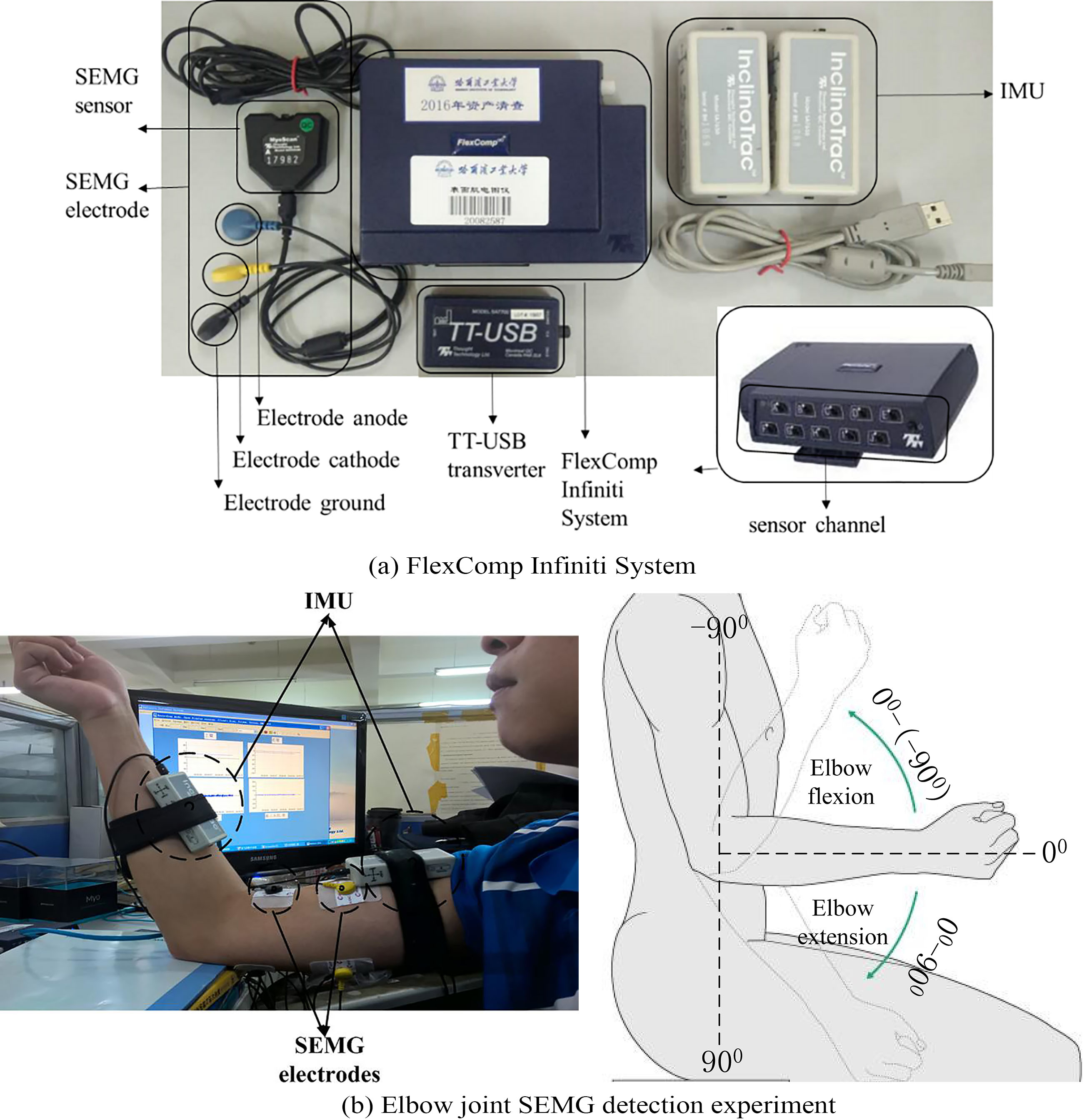
Figure 2.
Elbow joint signals of subject 1.
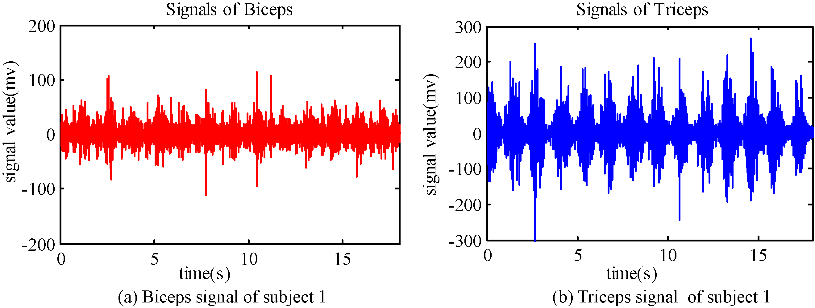
Take the subject 1 as an example, one set of SEMG experimental data is shown in Fig. 2. Where, (a) is the biceps signal of subject 1, (b) is the triceps signal of subject 1. It can be seen in the figures that biceps and triceps muscle in the antagonistic state in the elbow joint flexion/extension process.
2.2SEMG features extraction
Take a number every seven data in a same set of data and get a total of 8000 data. Applied a rectangular window of length 3000 in the signal process and modeling utilized MATLAB software.
Usually, the extracted features of the SEMG signals mainly are time domain, frequency domain and time-frequency or time-scale representation. Phinyomark et al. [4] extracted 37 SEMG features, and compared their performance in EMG signal classification. The results presented that features in time-domain showed better performance, therefore, mean absolute value (MAV), waveform length (WL), variance of EMG (VAR) and root mean square (RMS) were selected to be the features in this study.
(1)
Where, MVAB, WLB, VARB, RMSB are respectively the MAV, WLB, VARB, and RMSB of the biceps, MVAT, WLT, VART, RMST are respectively the MAV, WLB, VARB, and RMSB of the triceps.
2.3Principal Component Analysis (PCA)
Principal Component Analysis (PCA) adopts an orthogonal transformation to transform a set of observations of possibly correlated variables into a set of linearly uncorrelated values of variables which were called principal components. And the number of the principle components is less than or equal to the number of original variables. The largest possible variance is the first principal component of PCA, and each succeeding component in turn has the highest variance possible under the constraint that it is to the preceding components. Although four features in time-domain were selected to represent the SEMG of the biceps and triceps, an 8-dimension matrix still lead to a relatively large amount of calculation.
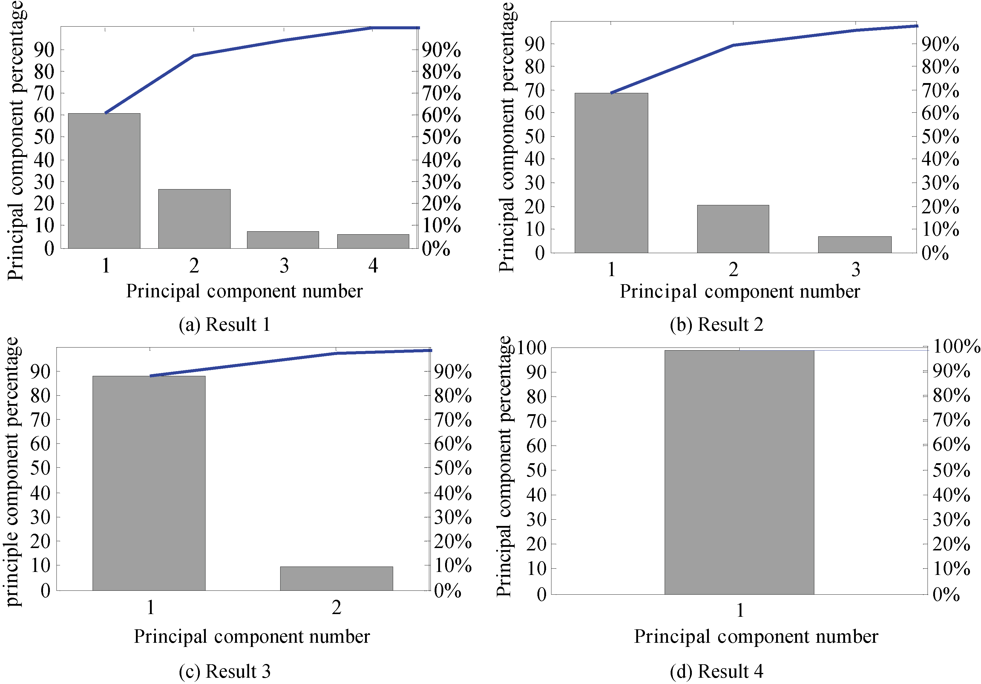
In the study, the PCA method was utilized to reduce the dimension of the Feature matrix (expression (5)) which is an 8-dimension matrix. A lower dimension feature matrix was achieved after the analysis, Fig. 3 shows the analysis result of PCA. It indicated that the 4-dimension, 3-dimension, 2-dimension, 1-dimension principal components respectively reflected the 8-dimension features almost completely under different data analysis results. In Fig. 3a–d, x-axis represented the principal component number after the analysis; y-axis represented the percentage of information of each principle components, equivalently, the information contained in each principal component accounts for the proportion of all information. It can be seen that the result of the percentage of the 4 or 3 or 2 or 1 principle components add together can almost completely represented the 8-dimendion features. Figure 4 shows the features after PCA analysis, which corresponds to the PCA results of Fig. 3, and the Fig. 4a–d shows the principal components of the different sets of data after analysis, which respectively is a linear combination of the old 8-dimension features.
Figure 3.
PCA analysis results.
3.BP model and RBF model of SEMG-angle
The model accuracy
(2)
(3)
Where,
3.1SEMG-angle model of BP neural networks
Figure 5 shows the structure of BP network model, and the method was used to determine the model parameters. The SEMG features of biceps and triceps was the input information which was a 4-dimension matrix after dimension reduction with PCA method. The training and testing data were respectively entered into the BP network.
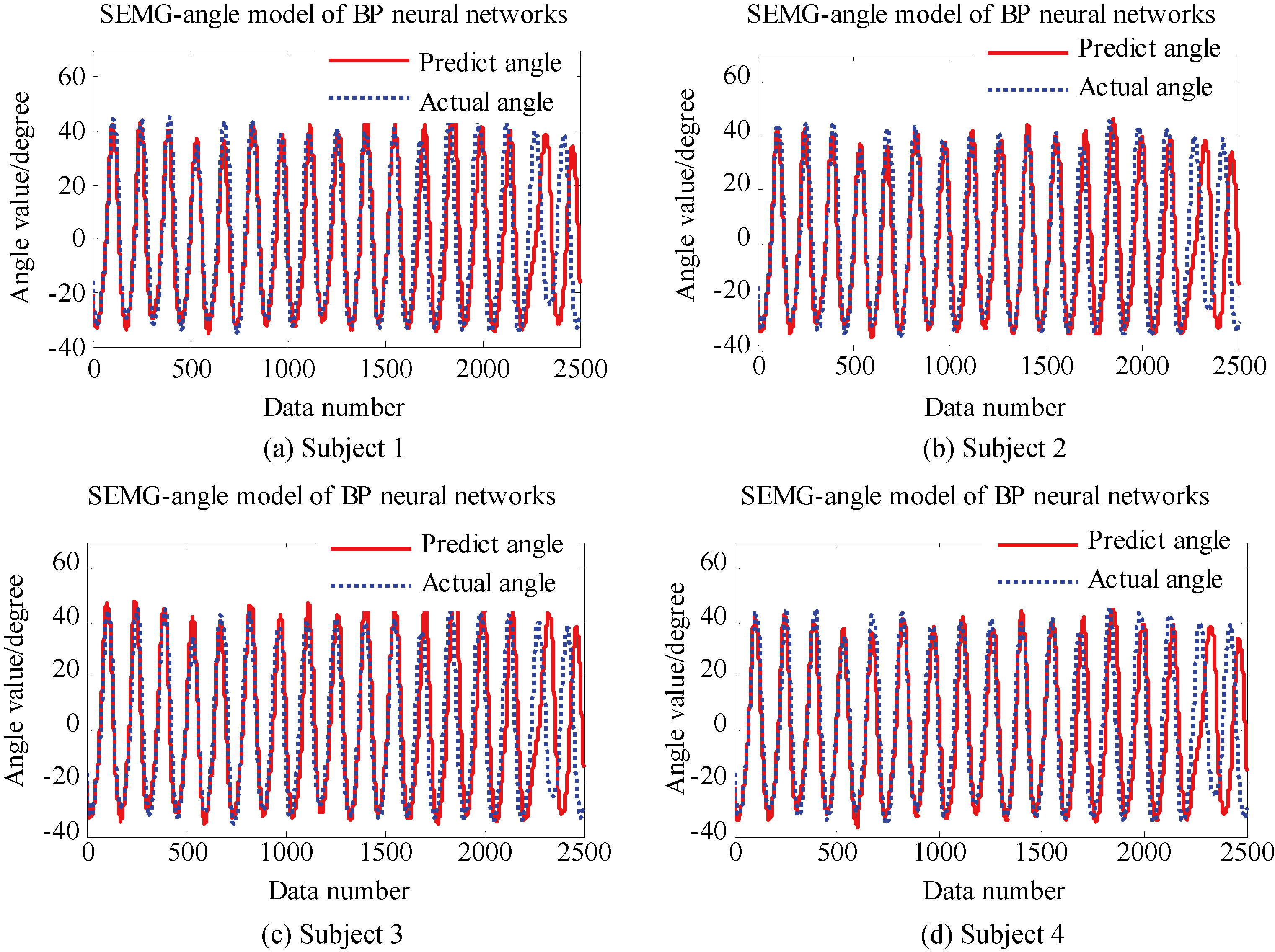
To avoid the excessive repeatability, take a set of four subjects’ modeling results for instructions. Figure 6 shows the results of predict angle and actual angle based on BP model. After extracting the features by applying a rectangular to the 8000 data points, each set has a total of 5000 data points. Each set of data is divided into two parts, one for establishing the SEMG-angle and the other for angle prediction.
The average accuracy of BP model was 88.180%, which is shown in Table 1. There are a total of 24 sets of test data with eight subjects, and three experiments per person. Where,
Table 1
The accuracy of BP model
| Experiment 1 | Experiment 2 | Experiment 3 | BP | |
|---|---|---|---|---|
| Subject 1 | 86.328% | 88.141% | 88.068% | 88.180% |
| Subject 2 | 88.655% | 89.663% | 86.667% | |
| Subject 3 | 87.121% | 89.242% | 88.339% | |
| Subject 4 | 87.204% | 86.621% | 87.802% | |
| Subject 5 | 88.163% | 88.104% | 87.321% | |
| Subject 6 | 89.086% | 89.972% | 90.008% | |
| Subject 7 | 87.399% | 89.002% | 88.511% | |
| Subject 8 | 88.633% | 88.001% | 88.267% |
Figure 4.
Features after PCA analysis.
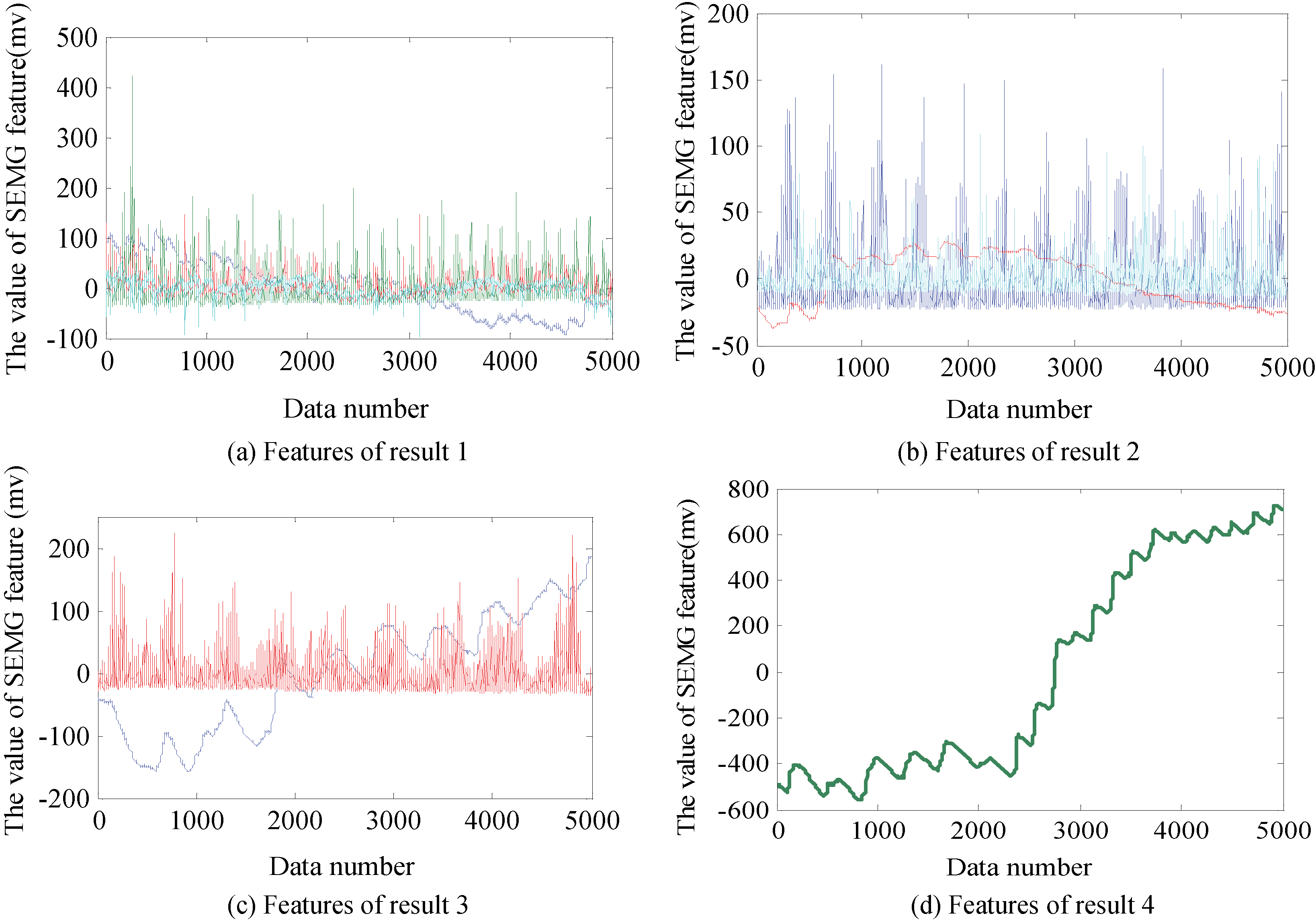
Figure 5.
Structure of BP model.
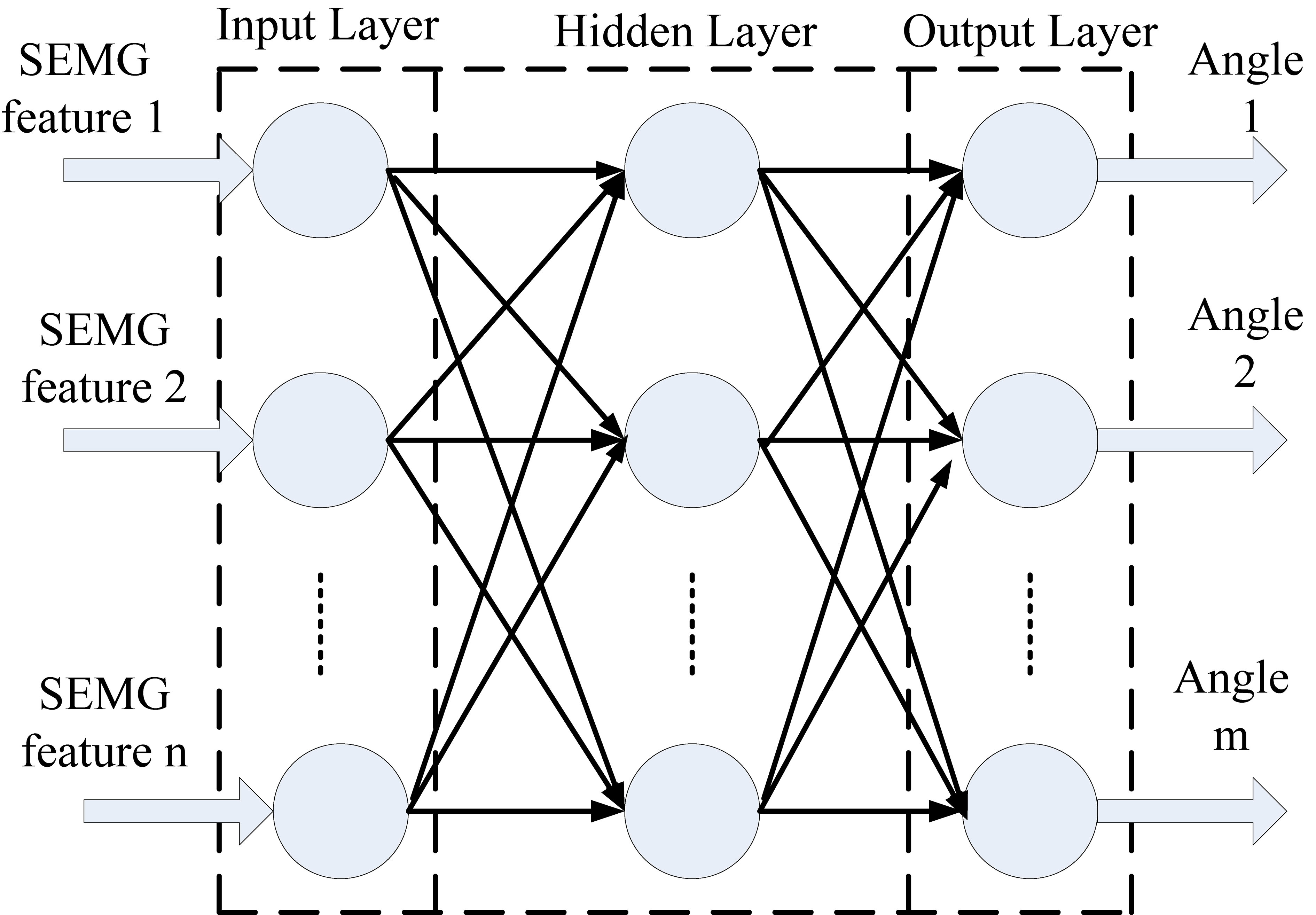
Figure 6.
SEMG-angle model of BP neural networks.
3.2SEMG-angle model of RBF neural networks
Figure 7 shows the structure of RBF network model, the function applied between the input layer and radial base artificial neural layer (hidden layer) was Gaussian function, and linear transformation was applied between the output layer and radial base artificial neural layer (hidden layer).
Figure 7.
Structure of RBF model.
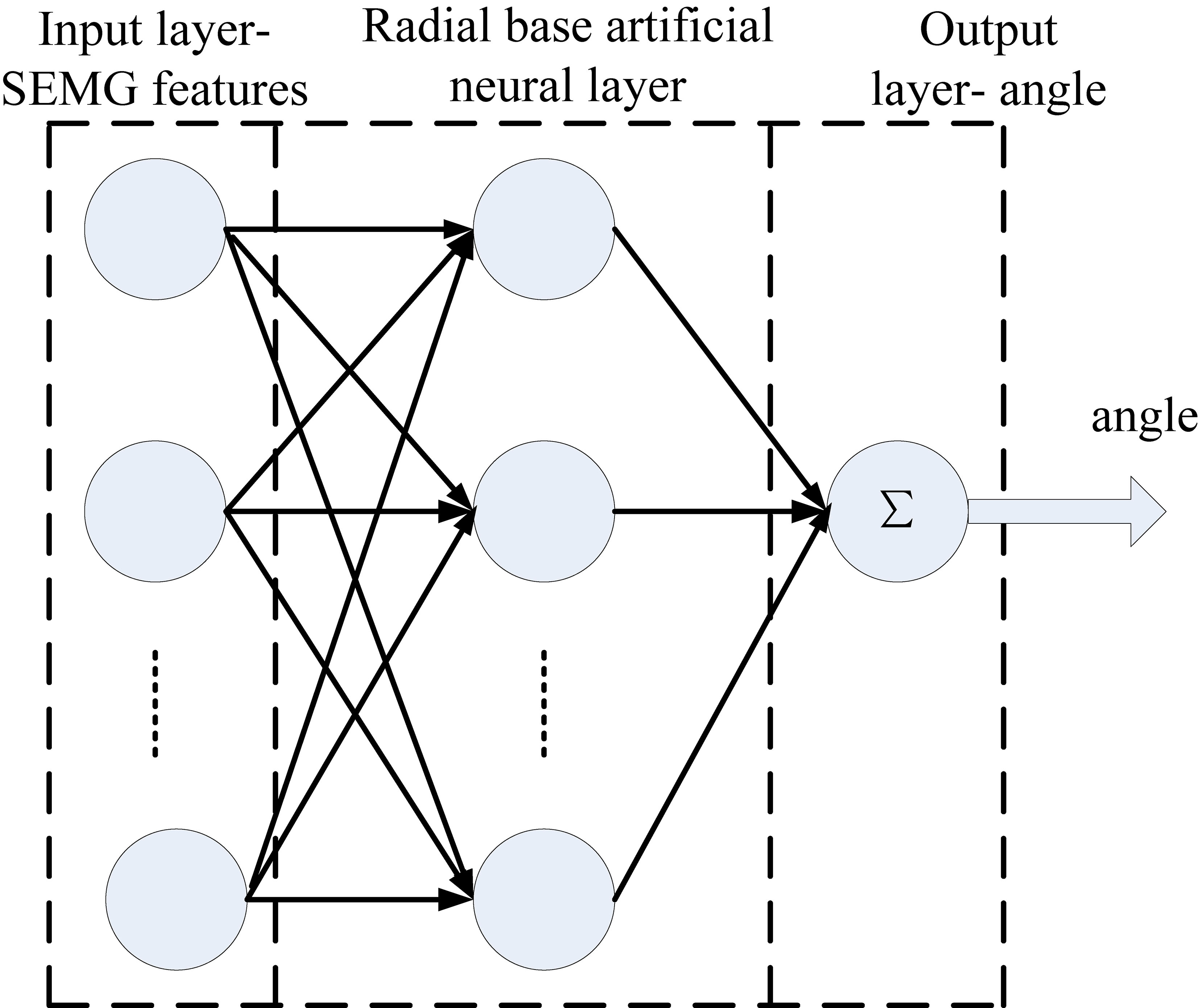
Figure 8.
SEMG-angle model of RBF neural networks.
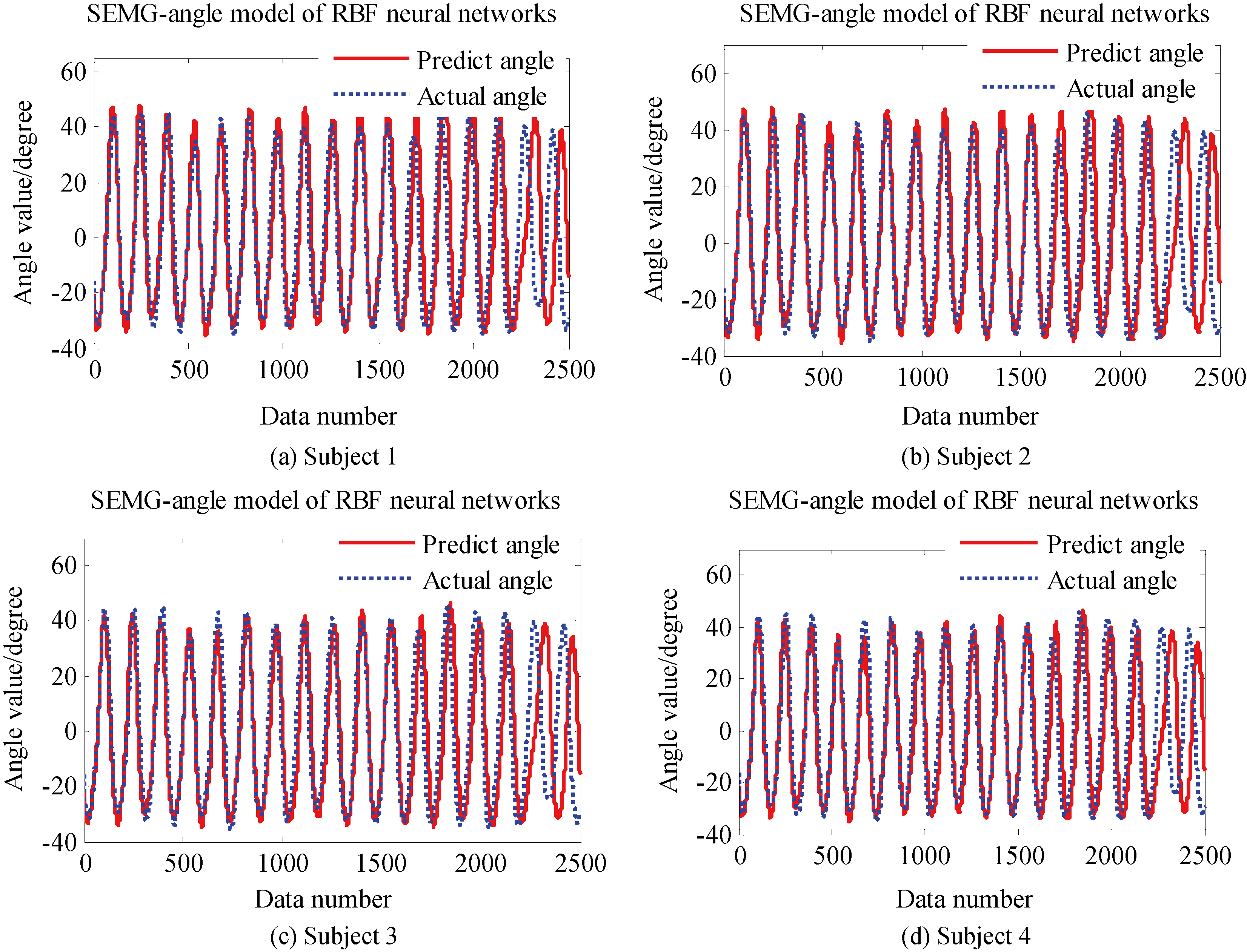
The predict results of predict angle and actual angle based on RBF model were shown in Fig. 8. Data used in RBF neural networks modeling is the same as the BP neural network. 5000 data points for each set of experiment are divided into two parts, one for establishing the SEMG-angle and the other for angle prediction.
The RBF model average accuracy was 88.752%, which is shown in Table 2. There are a total of eight subjects, three experiments per person. Where,
Table 2
The accuracy of RBF model
| Experiment 1 | Experiment 2 | Experiment 3 | RBF | |
|---|---|---|---|---|
| Subject 1 | 88.684% | 88.253% | 87.892% | 88.752% |
| Subject 2 | 89.021% | 88.717% | 88.545% | |
| Subject 3 | 88.337% | 88.700% | 89.301% | |
| Subject 4 | 88.986% | 89.019% | 89.113% | |
| Subject 5 | 89.106% | 87.998% | 88.529% | |
| Subject 6 | 88.667% | 88.693% | 89.009% | |
| Subject 7 | 88.233% | 88.958% | 88.771% | |
| Subject 8 | 89.215% | 89.097% | 89.200% |
4.HMM of SEMG-angle
The structure of Hidden Markov Model (HMM) is shown in Fig. 9. HMM is a statistical model, used to describe a hidden unknown parameters of the Markov process. The state in HMM is invisible, and what can be seen is the probability function of the observed value and the state. The HMM model is a double stochastic process in which the observed value is a stochastic process with respect to the state, and the state is a stochastic process with respect to time.
Figure 9.
Structure of Hidden Markov Model.
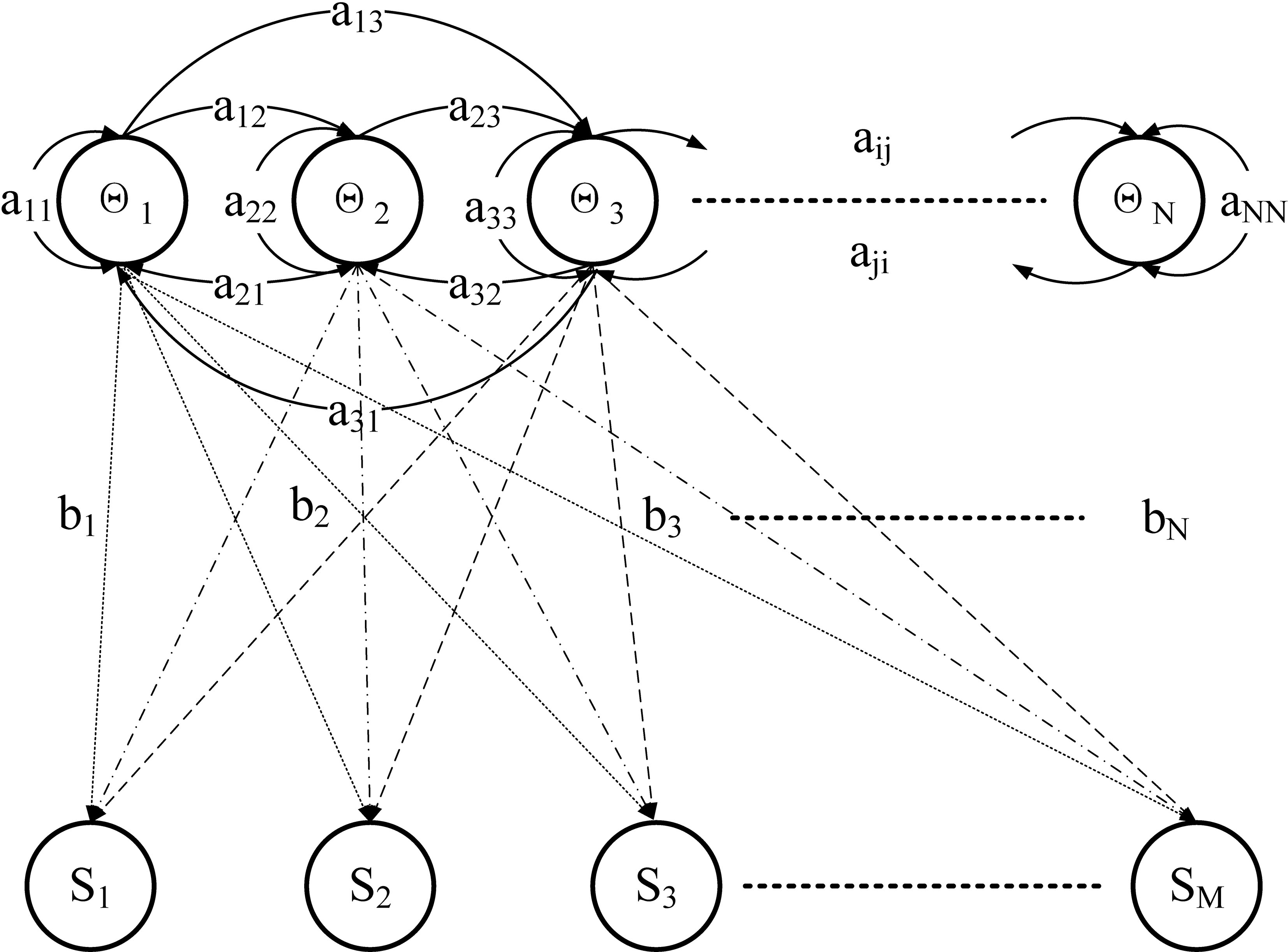
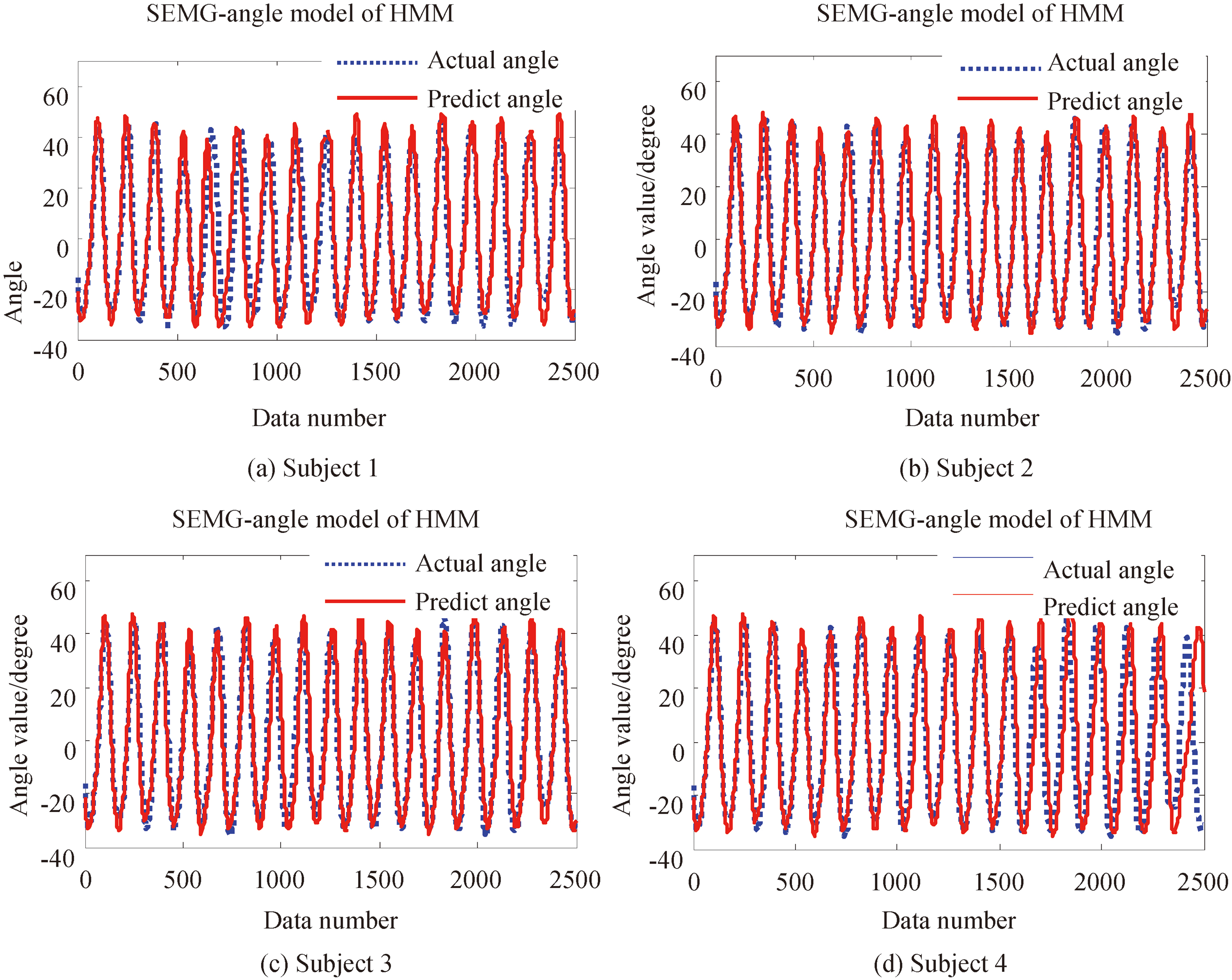
Figure 10.
SEMG-angle model of HMM.
There are
(4)
(5)
where,
(6)
HMM is based on three assumptions: the state constitutes the first order Markov chain; state has nothing to do with the specific time; the output is only relevant to the current state. HMM can solve the problem of randomly generating surface events by potential causes.
Because of the serial number representation of the HMM model, the training and testing data were numbered accordingly before entered into the model. The training data were applied to establish the HMM model and identify the state transition probability
HMM model average accuracy can reach about 93.063% which is shown in Table 3. Where,
Table 3
The accuracy of HMM model
| Experiment 1 | Experiment 2 | Experiment 3 | HMM | |
|---|---|---|---|---|
| Subject 1 | 90.802% | 93.267% | 93.159% | 93.063% |
| Subject 2 | 93.222% | 92.884% | 92.467% | |
| Subject 3 | 94.011% | 93.977% | 92.852% | |
| Subject 4 | 92.993% | 93.991% | 93.878% | |
| Subject 5 | 93.156% | 91.898% | 93.013% | |
| Subject 6 | 93.211% | 92.966% | 93.257% | |
| Subject 7 | 92.989% | 93.051% | 93.244% | |
| Subject 8 | 93.111% | 93.200% | 92.907% |
5.Discussion and conclusion
As it was mentioned above, HMM model accuracy of SEMG-angle achieved an average value of 93.063%, and it exceeded the BP method (88.180%) and RBF method (88.752%) applied before. A comparison table was given to show the different performance of various EMG-angle model separately based on BP, RBF and HMM model. The results were shown in Table 4. It can be seen in Table 4: all three methods can be used to solve the nonlinear relationship modeling, BP network structure is simple when solving this modeling problem, and has the similar performance compared with RBF model. Both of the neural network can achieve a good prediction at the beginning, however the result was not very stable with the increase of the data number. BP network training results can easily be limited to the local minimum, while RBF can be globally approximated. Nevertheless, the performance of HMM model was relatively stable and the predict angle with HMM model were closer to the actual elbow joint angle.
Table 4
Modeling results comparison of HMM BP and RBF neural networks
| Modeling principles | Average | Offline | Structure | Others | |
| accuracy | modeling | ||||
| time | |||||
| HMM | Probability problem of stochastic process statistical characteristics | 93.063% | 3–5 s | Discrete state, the input and output are probabilistic | Each state depends on the previous state and the transition probability |
| BP | Solve the nonlinear mapping relationship | 88.180% | 1.5–3 s | 3 layers or more, local optimum | The activation function is the S function, and the learning rate is fixed |
| RBF | Solve the nonlinear mapping relationship | 88.752% | 5–8 s | 3 layers, global approximation | The activation function is a Gaussian function, and the generalization ability is better than BP network |
HMM method is different from neural network in principle, and it is suitable for solving the probability mapping relationship between input and output of double random process. To a certain extent, HMM method can be seen as a layer 2 network. The hidden layer and the output layer are visible, there is a state transition probability between each state, and there is a visible layer state probability observed between the hidden layer and the output visible layer due to the hidden layer state. Because of the inherent characteristic properties that current results and states are biased toward the previous results and states in HMM method, the method can eliminate spurious misclassification and modeling [10]. The application of HMM was mainly involved pattern recognition, and few studies about model based on this method. In consideration of the similarity about pattern recognition and SEMG-angle modeling, an SEMG-angle model based on HMM was proposed in this study.
The HMM training process developed an angle library and it can be built offline. The modeling and training time of HMM method with fewer calculations and it is computationally comparable to BP and RBF method, and also the HMM method proposes a massive computational savings on testing time compared to BP and RBF method. The low computational overhead associated with HMM model makes it is possible to predict the continuous angle.
In order to improve the accuracy of modeling prediction, we will conduct in-depth research on SEMG signals with the study of different characteristics of SEMG which attempt to uncover the deeper relationship between SEMG and joint angles. Additional work about the research on SEMG at the same joint angles, combined some new algorithms to improve the accuracy of modeling prediction and real-time prediction of joint angle in HRI for rehabilitation exoskeleton system will be our future work.
Acknowledgments
The work reported in this paper was funded by the Natural Science Foundation of Jiangsu Province (Grant no. BK20180270).
Conflict of interest
None to report.
References
[1] | Ahsan MR, Ibrahimy MI, Khalifa OO. EMG signal classification for human computer interaction: a review. European Journal of Scientific Research, (2009) , 33: (3): 480-501. |
[2] | Boostani R, Moradi MH. Evaluation of the forearm EMG signal features for the control of a prosthetic hand. Physiological Measurement, (2003) , 24: (2): 309. https://doi.org/10.1088/0967-3334/24/2/307. |
[3] | Zecca M, Micera S, Carrozza MC, et al. Control of multifunctional prosthetic hands by processing the electromyographic signal. Critical ReviewsTM in Biomedical Engineering, (2002) , 30: (4-6). https://doi.org/10.1615/critrevbiomedeng.v30.i456.80. |
[4] | Phinyomark A, Phukpattaranont P, Limsakul C. Feature reduction and selection for EMG signal classification. Expert Systems with Applications, (2012) , 39: (8): 7420-7431. https://doi.org/10.1016/j.eswa.2012.01.102. |
[5] | Reed EB, Hanson AM, Cavanagh PR. Optimising muscle parameters in musculoskeletal models using Monte Carlo simulation. Computer Methods in Biomechanics and Biomedical Engineering, (2015) , 18: (6): 607-617. https://doi.org/10.1016/j.eswa.2012.01.102. |
[6] | Han J, Ding Q, Xiong A, et al. A state-space EMG model for the estimation of continuous joint movements. IEEE Transactions on Industrial Electronics, (2015) , 62: (7): 4267-4275. https://doi.org/10.1109/tie.2014.2387337. |
[7] | Wang S, Gao Y, Zhao J, et al. Prediction of sEMG-based tremor joint angle using the RBF neural network// In: 2012 IEEE International Conference on Mechatronics and Automation. IEEE, (2012) : pp. 2103-2108. https://doi.org/10.1109/icma.2012.6285668. |
[8] | Mesa I, Rubio A, Tubia I, et al. Channel and feature selection for a surface electromyographic pattern recognition task. Expert Systems with Applications, (2014) , 41: (11): 5190-5200. https://doi.org/10.1016/j.eswa.2014.03.014. |
[9] | Chan ADC, Englehart KB. Continuous myoelectric control for powered prostheses using hidden Markov models. IEEE Transactions on Biomedical Engineering, (2005) , 52: (1): 121-124. https://doi.org/10.1109/tbme.2004.836492. |
[10] | Huang Y, Englehart KB, Hudgins B, et al. A Gaussian mixture model based classification scheme for myoelectric control of powered upper limb prostheses. IEEE Transactions on Biomedical Engineering, (2005) , 52: (11): 1801-1811. https://doi.org/10.1109/tbme.2005.856295. |
[11] | Hargrove LJ, Li G, Englehart KB, et al. Principal components analysis preprocessing for improved classification accuracies in pattern-recognition-based myoelectric control. IEEE Transactions on Biomedical Engineering, (2009) , 56: (5): 1407-1414. https://doi.org/10.1109/tbme.2008.2008171. |
[12] | Khezri M, Jahed M. A neuro-fuzzy inference system for sEMG-based identification of hand motion commands. IEEE Transactions on Industrial Electronics, (2011) , 58: (5): 1952-1960. https://doi.org/10.1109/tie.2010.2053334. |
[13] | Bu N, Okamoto M, Tsuji T. A hybrid motion classification approach for EMG-based human-robot interfaces using bayesian and neural networks. IEEE Transactions on Robotics, (2009) , 25: (3): 502-511. https://doi.org/10.1109/tro.2009.2019782. |
[14] | Duan F, Dai L, Chang W, et al. sEMG-based identification of hand motion commands using wavelet neural network combined with discrete wavelet transform. IEEE Transactions on Industrial Electronics, (2016) , 63: (3): 1923-1934. |
[15] | Cao H, Boudaoud S, Marin F, et al. Surface EMG-force modelling for the biceps brachii and its experimental evaluation during isometric isotonic contractions. Computer Methods in Biomechanics and Biomedical Engineering, (2015) , 18: (9): 1014-1023. https://doi.org/10.1080/10255842.2013.867952. |
[16] | Meattini R, Benatti S, Scarcia U, et al. An sEMG-based human-robot interface for robotic hands using machine learning and synergies. IEEE Transactions on Components, Packaging and Manufacturing Technology, (2018) , 8: (7): 1149-1158. |
[17] | Li C, Zhou Y, Li Y. The signal processing and identification of upper limb motion based on sEMG. Wireless Personal Communications, (2018) , 103: (1): 887-896. https://doi.org/10.1007/s11277-018-5485-z. |


