
An automatic glioma grading method based on multi-feature extraction and fusion
Abstract
BACKGROUND:
An accurate assessment of tumor malignancy grade in the preoperative situation is important for clinical management. However, the manual grading of gliomas from MRIs is both a tiresome and time consuming task for radiologists. Thus, it is a priority to design an automatic and effective computer-aided diagnosis (CAD) tool to assist radiologists in grading gliomas.
OBJECTIVE:
To design an automatic computer-aided diagnosis for grading gliomas using multi-sequence magnetic resonance imaging.
METHODS:
The proposed method consists of two steps: (1) the features of high and low grade gliomas are extracted from multi-sequence magnetic resonance images, and (2) then, a KNN classifier is trained to grade the gliomas. In the feature extraction step, the intensity, volume, and local binary patterns (LBP) of the gliomas are extracted, and PCA is used to reduce the data dimension.
RESULTS:
The proposed "Intensity-Volume-LBP-PCA-KNN" method is validated on the MICCAI 2015 BraTS challenge dataset, and an average grade accuracy of 87.59% is obtained.
CONCLUSIONS:
The proposed method is an effective method for automatically grading gliomas and can be applied to real situations.
1.Introduction
Every year, primary malignant brain tumor cases are widely diagnosed in the world [1]. A common type of brain tumor is glioma, which accounts for up to 30% of all brain and central nervous system (CNS) tumors and 80% of all malignant brain tumors [2]. Glioma severity is further distinguished by grades ranging from least malignant (I) to most malignant (IV), according to such features as atypical cellular characteristics, cell proliferation, angiogenesis, and necrosis [3]. Grades I and II gliomas are considered low grade tumors, whereas Grades III and IV gliomas are considered high grade tumors [4]. For low grade tumors, the prognosis is somewhat more optimistic; the median survival of patients diagnosed with a low grade glioma is 11.6 years [5]. In contrast, the median overall survival of patients with high grade glioma is approximately 3 years. More seriously, glioblastoma multiform is a type of high grade glioma that has a poor median overall survival of 15 months [6].
Clinical management is dependent upon an accurate assessment of tumor malignancy grade in the preoperative situation [4]. Magnetic resonance imaging (MRI) is the method of choice for the radiological evaluation of brain tumors. As a rapid and non-invasive imaging technique, MRIs allow for an investigation of the anatomic structure of both healthy and diseased brains as well as provide considerable information for glioma diagnosis. However, the process of manually grading gliomas from numerous MRIs it is a very tiresome and time-consuming task for radiologists. Thus, the development of an automatic and effective computer-aided diagnosis (CAD) tool would be a significant asset to radiologists for the process of grading gliomas.
At present, numerous methods have been proposed for automatic diagnosis. The majority of these methods consist of two steps: feature extraction and classification. Feature extraction utilizes an initial set of measured data and builds derived features that are intended to be informative and non-redundant; this facilitates the subsequent learning and generalization steps and, in some cases, leads to better human interpretations [7]. For MR image classification, the intensity features, shape features, and texture features are always extracted to describe the differences between normal regions and abnormal regions in the brain. In previous works, features such as histogram, mean value, variance, area, perimeter, circularity, irregularity, contrast, entropy, SIFT [8], HOG [9], WLD [10], DWT [11], and D-HLDO [12, 13] were usually extracted for biometric image classification. After the feature extraction, the classification model is used. Frequently used classification patterns include fuzzy C-means (FCM) [14], Gaussian mixture model (GMM) [15], K-nearest neighbors (KNN) [16], support vector machine (SVM) [17, 18, 19], random forest (RF) [20], sparse representation-based classifier [21], and so on.
In this paper, the aim is to develop an accurate gliomas grade system. Therefore, we propose an automatic computer-aided diagnosis to grade the gliomas obtained by multi-sequence magnetic resonance imaging. The proposed method consists of two steps: (1) the intensity, volume, and LBP features of high grade and low grade gliomas are extracted from multi-sequence magnetic resonance images. Then, principle component analysis (PCA) is used to reduce the dimension and combine the features. (2) Using the fusion feature, a KNN classifier is trained to grade the testing gliomas. The proposed “Intensity-Volume-LBP-PCA-KNN” method is validated on the MICCAI 2015 BraTS challenge dataset (http://braintumorsegmentation.org/), and an average grade accuracy of 87.59% is obtained. The proposed method is effective and can be applied for practical use.
2.Data description
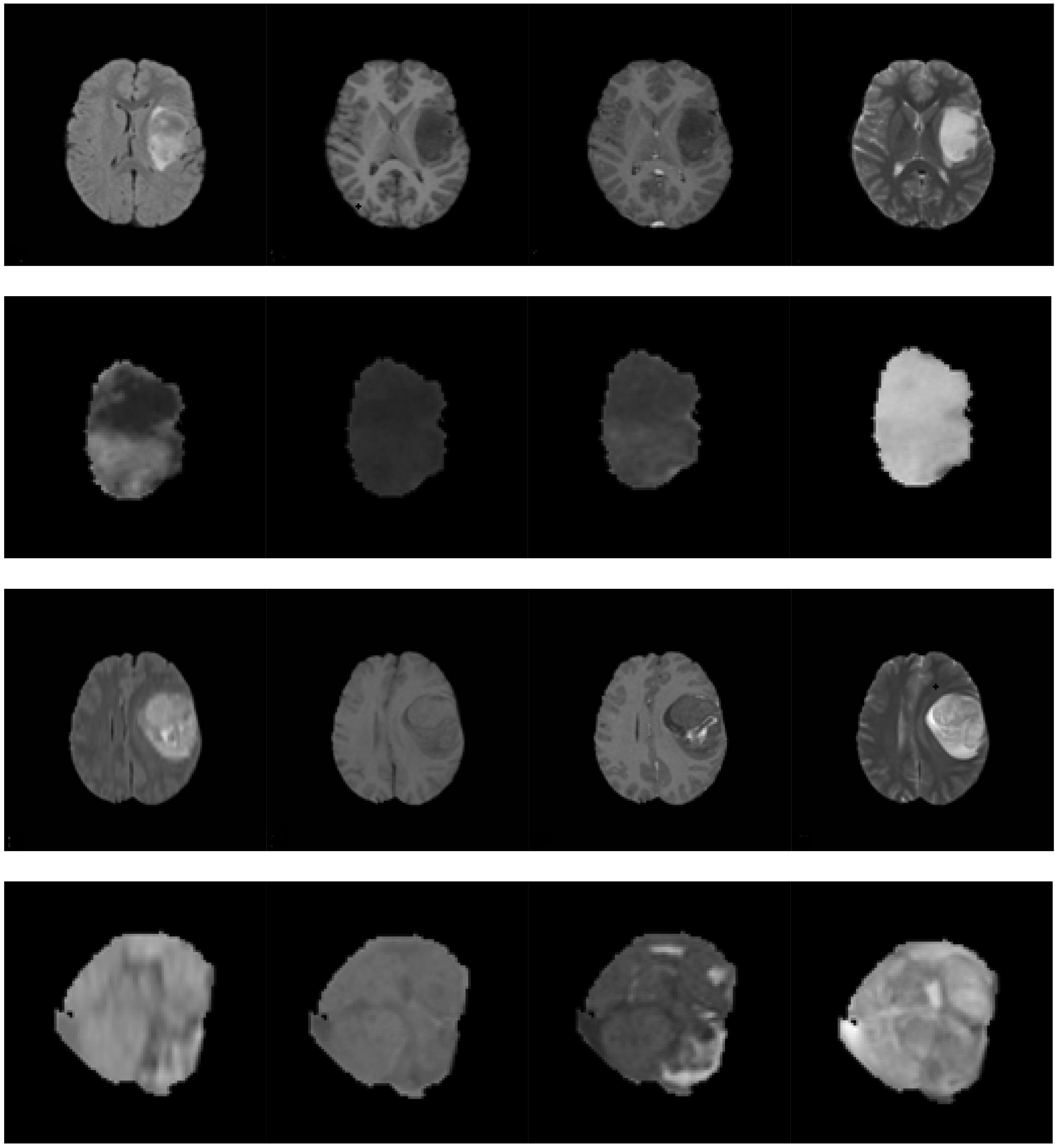
For glioma grading, multi-sequence MRIs are frequently used for tumor assessment. The following sequences are commonly applied: T1-w, T2-w, FLAIR, and T1-w with contrast enhancement (T1-wc). Figure 1 shows the multi-sequence MRIs of low grade and high grade gliomas, respectively. In the T1-w MRI, healthy tissues are easily distinguishable. Moreover, the T1-wc MRI provides a clear difference between the necrotic core and the active cell region. In the T2-w MRI, the intensities of the edema and tumor regions are higher than those of normal tissues. The differences between CSF and lesions are highly obvious [22] in the FLAIR MRI. Therefore, a fusion of the information from the multi-sequence MRIs is required to accurately grade gliomas.
Figure 1.
Multi-sequence MRIs of the low grade glioma and high grade glioma. The first through last rows are as follows: (1) the multi-sequence MRIs of the low grade glioma; (2) the tumor region extracted from the images in the first row; (3) the multi-sequence MRIs of the high grade glioma; and (4) the tumor region extracted from the images in the third row. The first through last columns are as follows: FLAIR sequence, T1-w sequence, T1-wc sequence, and T2-w sequence, respectively.
3.Feature extraction and fusion
Before feature extraction, the MRIs were pre-processed in three steps: nonparametric intensity non-uniformity normalization (N3-correction), tumor segmentation, and image re-slicing. N3-correction corrects the inhomogeneity in each set of MRI scans [23]. Tumor segmentation was conducted in order to classify the MRIs into enhancing tumor, non-enhancing tumor, necrosis, edema, and normal tissues. The MICCAI 2015 BraTS challenge dataset provides the segmentation ground truth of each case. The image slice with the maximum tumor area was extracted from each MRI sequence for 2D texture features.
4.Intensity feature
The intensity feature is one of the most widely used features. In the proposed method, we extracted seven intensity features of the 3D tumor region in each MRI sequence: the greatest intensity value, smallest intensity value, mean intensity value, median intensity value, the intensity at the histogram peak, the intensity at the histogram valley, and the variance of the tumor region. Therefore, the intensity feature of one case is a vector with 28 elements.
4.1Volume feature
From Fig. 1, it can be seen that the volumes of the low grade glioma and high grade glioma are quite different. We extracted the volumes of the enhancing tumor, non-enhancing tumor, necrosis, edema, complete tumor, and the whole outlier region (including the tumor region and edema region) as the volume feature. According to this extraction, the volume feature of each case is a vector with 6 elements.
4.2Texture feature
Texture is an image characteristic that provides a higher order description of an image and includes information about the spatial distribution of intensity [24]. The texture extraction defines the homogeneity or similarity between regions of an image. From Fig. 1, the homogeneity of the tumor region in the T1-wc sequence is very different for thelow grade glioma and compared to the high grade glioma. In the proposed method, the LBP method was applied to extract the texture feature. The LBP operator assigned a label to every pixel of an image by thresholding the 3
4.3Feature fusion and dimension reduction
The intensity feature, volume feature, and texture feature were combined to form a complete glioma feature, which is a vector containing 289 elements. Then, PCA was used to approximate the complete feature set with lower dimensional feature vectors. The principal components are the projections of the original features onto the eigenvectors, which correspond to the largest eigenvalues of the covariance matrix of the original feature set. The first L principal components were used for classifier training and testing.
5.Classification using KNN
After dimension reduction, the features were submitted to the classification procedure. A KNN cla-ssifier was used to determine the glioma grade. The input of the KNN classifier consists of the k closest training samples in the feature space, and the output of the KNN classifier is a class membership. A testing sample was classified by a majority vote of its neighbors, with the testing sample being assigned to the class most common among its k nearest neighbors. In our application, the class number k is 2, as we only need to estimate whether a glioma is low grade or high grade.
6.Experimental results
The MICCAI 2015 BraTS challenge data set was used for our method validation and experimental comparison. All of the data from the challenge database was provided by ETH Zurich, University of Bern, University of Debrecen, and University of Utah [26]. It contains 220 HGG cases and 54 LGG cases. All brains in the datasets have the same orientation. For each brain, all available sequences, i.e., T1-w, T1-wc, T2-w, and FLAIR sequences, were already co-registered and provided with ground truth. The ground truth of the data was subdivided into enhancing tumor, non-enhancing tumor, necrosis, and edema. Before classification was performed, all features were normalized into [0, 1].
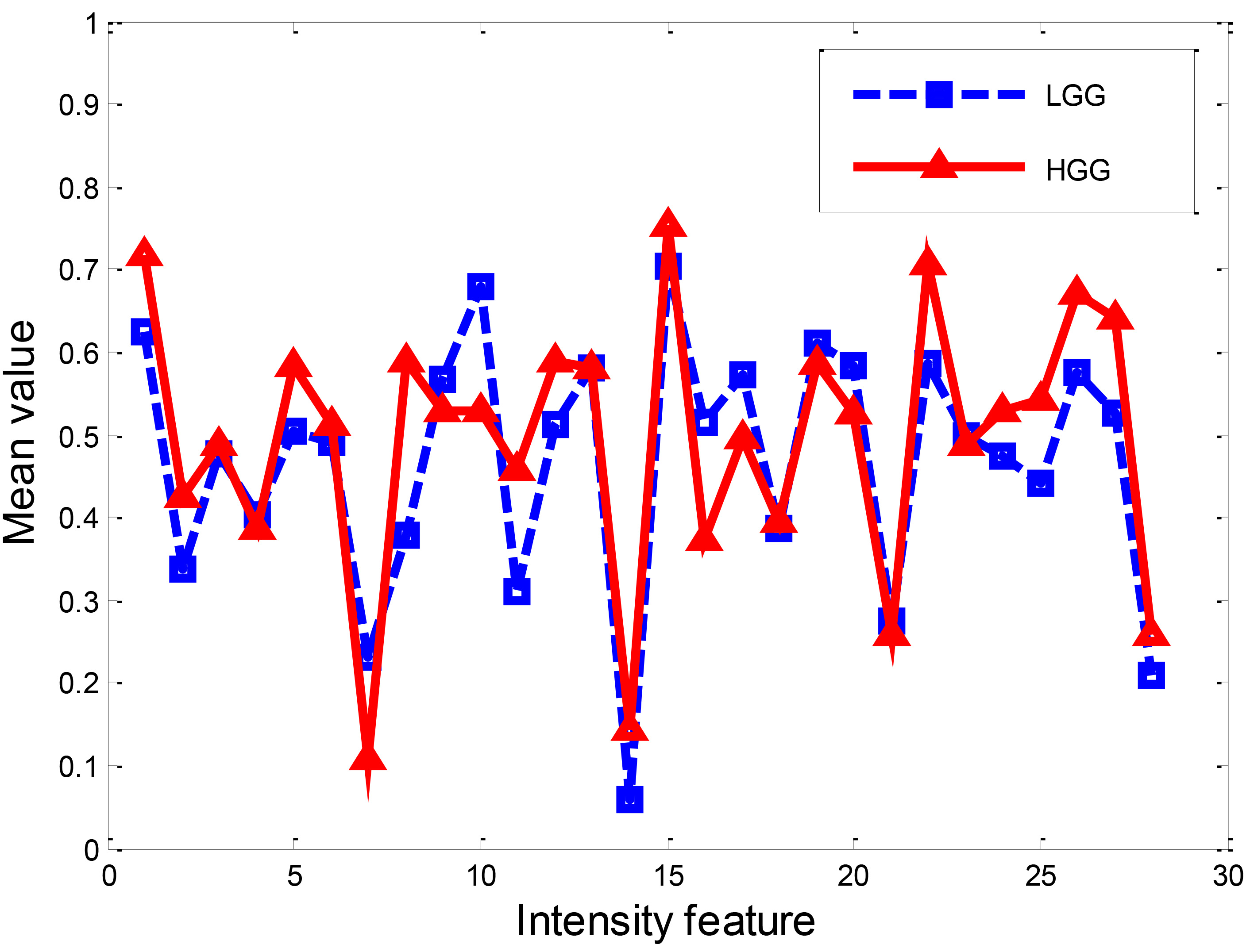
6.1Intensity feature extraction result
First, intensity feature extraction was carried out on both the LGG and HGG datasets, respectively. Figure 2 demonstrates the mean value of the intensity feature extracted from LGG and HGG, respectively. From the figure, it is clear that some of the intensities of HGG and LGG are quite different.
Figure 2.
Intensity feature of LGG and HGG.
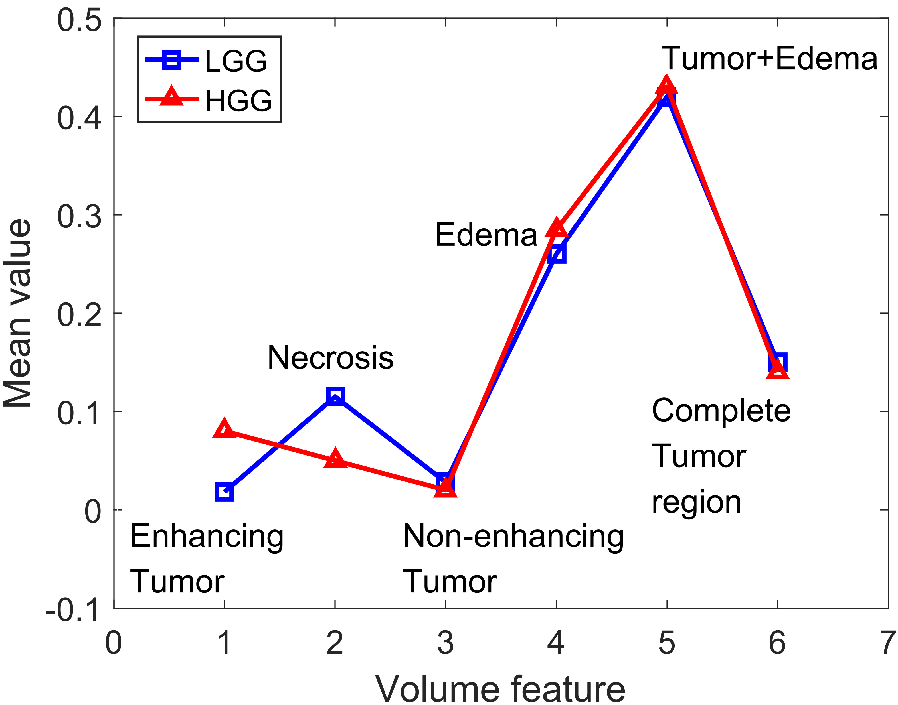
6.2Volume feature extraction result
Next, we calculated the volume feature of LGG and HGG, respectively. The mean values of the corresponding regions of LGG and HGG are shown in Fig. 3. From the figure, it can be seen that the enhancing tumor volume of HGG is greater than that of LGG, whereas the necrosis volume of LGG is greater than that of HGG, and the volumes of the other parts are very close.
Figure 3.
Volume feature of LGG and HGG.
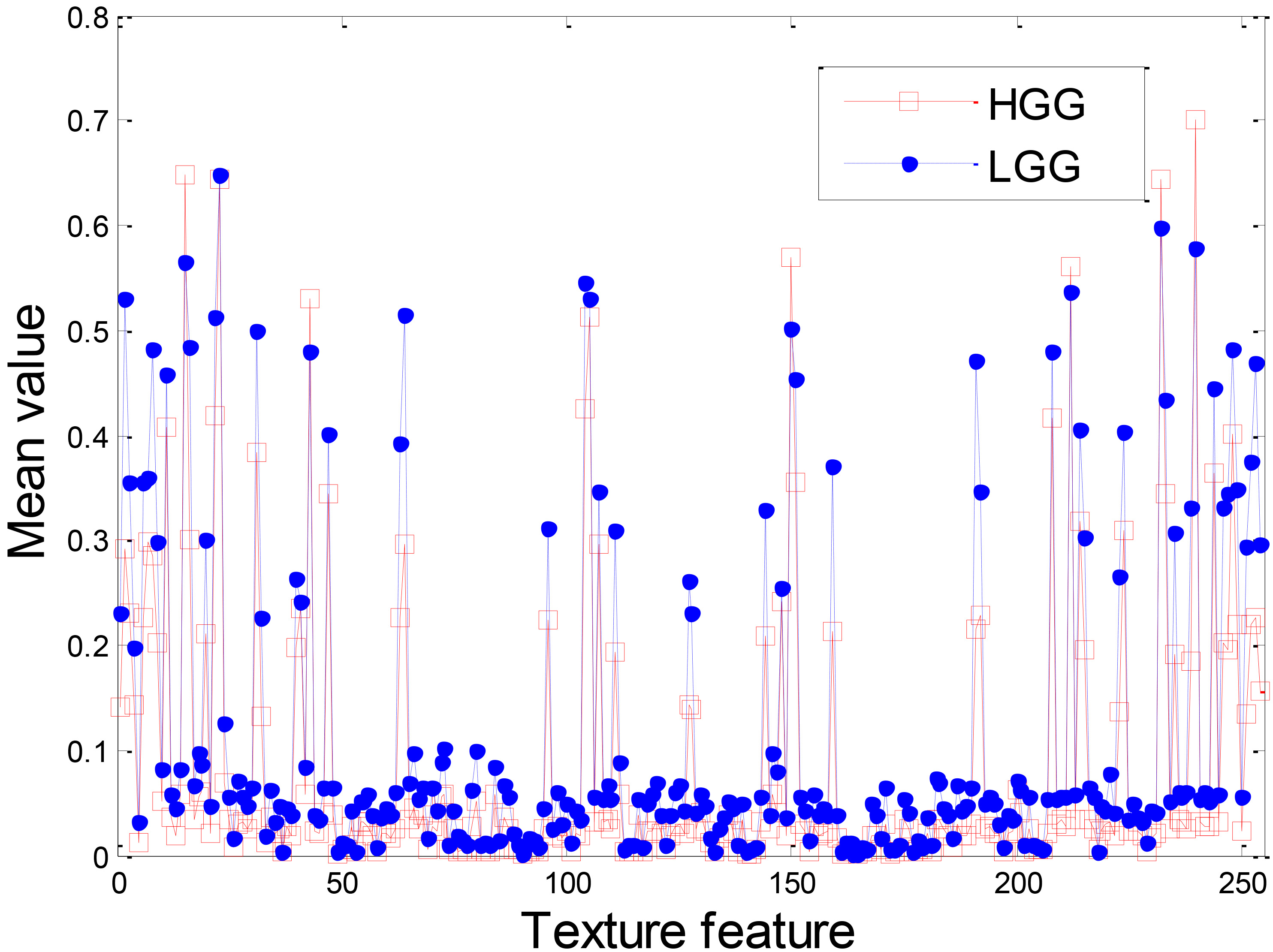
6.3Texture feature extraction result
Figure 4 demonstrates the texture feature of LGG and HGG. Although the overall shapes of the texture feature extracted from LGG and HGG are similar, there is a large gap between some of the LGG texture feature values and the HGG texture feature values. This result indicates that the texture feature can be used for glioma grade.
6.4Classification results comparison
We compared the proposed method with the intensity-based method, volume-based method, texture-based method, and intensity-volume-based method. In our experiment, the training data of LGG and HGG were randomly selected from the whole dataset. The training data numbers of LGG and HGG are 10 and 40, respectively, because there are four times more HGG cases than LGG cases in the MICCAI 2015 BraTS challenge dataset. After dimension reduction, the first 120 principle components were used as the input data because the contribution rate of the first 120 principle components was more than 99%. We performed our method 10 times and calculated the mean value of the classification results. The overall accuracy was used for validation. The corresponding results are shown in Table 1. From the table, it can be seen that the accuracies of the Intensity-KNN method, Volume-KNN method, and Intensity-Volume-KNN method are very close and are a little higher than that of the Texture-KNN method. The accuracy of the grade results obtained by the proposed method is 2.3% higher than that of the Intensity-Volume-KNN method, 4.35% higher than that of the Texture-KNN method, 1.81% higher than that of the Volume-KNN method, and 2.21% higher than that of the Intensity-KNN method. This result indicates that feature fusion and dimension reduction play an important role in glioma grades.
Table 1
Classification accuracy comparison
| Methods | Overall accuracy (%) |
|---|---|
| Intensity-KNN | 85.40 |
| Volume-KNN | 85.77 |
| Texture-KNN | 83.24 |
| Intensity-Volume-KNN | 85.56 |
| Intensity-Volume-LBP-PCA-KNN | 87.59 |
Figure 4.
Texture feature of LGG and HGG.
7.Conclusion
To develop an effective and automatic method for grading gliomas from multi-sequence MRIs, we used multi-feature fusion and PCA to extract the original features and used KNN to classify the glioma into LGG and HGG. The experiments demonstrated that the proposed “Intensity-Volume-LBP-PCA-KNN” method superiorly graded gliomas from MICCAI 2015 BraTS dataset.
Conflict of interest
None to report.
Acknowledgments
The authors would like to thank the editors and the anonymous reviewers for their valuable comments and suggestions, which have were an immense help in improving the quality of this paper. This work is supported by the National Nature Science Foundation of China under Grant No.61502206 and 61473334; the Nature Science Foundation of Jiangsu Province under Grant No.BK20150523, 20150983, and BY2014007-04; the Open Project Program of Key Laboratory of Intelligent Perception and Systems for High-Dimensional Information of Ministry of Education (JYB201604); the Open Project of Jiangsu Key Laboratory of Meteorological Observation and Information Processing; Nanjing University of Information Science and Technology (KDXS1404); Jiangsu Postdoctoral Science Foundation Funded Project (No.1402094C); Research Foundation for Talented Scholars, Jiangsu University (No.14JDG041); and Open Project Program of Key Laboratory of Symbolic Computation and Knowledge Engineering of Ministry of Education, Jilin University (No.93K172016K17).
References
[1] | http://www.irsa.org/glioblastoma.html. |
[2] | Goodenberger MKL, Jenkins RB. Genetics of adult glioma. Cancer Genetics. (2012) ; 205: (12): 613-621. |
[3] | Sun Y, Zhang W, Chen D, et al. A glioma classification scheme based on coexpression modules of EGFR and PDGFRA. Proceedings of the National Academy of Sciences. (2014) ; 111: (9): 3538-3543. |
[4] | Michotte A, Neyns B, Chaskis C, et al. Neuropathological and molecular aspects of low-grade and high-grade gliomas. Actaneurologicabelgica. (2004) ; 104: (4): 148-153. |
[5] | Ohgaki H, Kleihues P. Population-based studies on incidence, survival rates, and genetic alterations in astrocytic and oligodendroglialgliomas. Journal of Neuropathology & Experimental Neurology. (2005) ; 64: (6): 479-489. |
[6] | Bleeker FE, Molenaar RJ, Leenstra S. Recent advances in the molecular understanding of glioblastoma. Journal of Neuro-Oncology. (2012) ; 108: (1): 11-27. |
[7] | https://en.wikipedia.org/wiki/Feature_extraction. |
[8] | Lowe DG. Distinctive image features from scale-invariant key points. International Journal of Computer Vision. (2004) ; 60: (2): 91-110. |
[9] | Dalal N, Triggs B. Histograms of oriented gradients for human detection, Computer Vision and Pattern Recognition, 2005. CVPR 2005. IEEE; Computer Society Conference on. IEEE. (2005) : 1: : 886-893. |
[10] | Chen J, Shan S, He C, et al. WLD: A robust local image descriptor. IEEE Transactions on Pattern Analysis and Machine Intelligence. (2010) ; 32: (9): 1705-1720. |
[11] | Zhang Y, Wang S, Phillips P, et al. Detection of Alzheimer’s disease and mild cognitive impairment based on structural volumetric MR images using 3D-DWT and WTA-KSVM trained by PSOTVAC. Biomedical Signal Processing and Control. (2015) ; 21: : 58-73. |
[12] | Qian J, Yang J, Xu Y. Local structure-based image decomposition for feature extraction with applications to face recognition. IEEE Transactions on Image Processing. (2013) ; 22: (9): 3591-3603. |
[13] | Qian J, Yang J, Gao G. Discriminative histograms of local dominant orientation (D-HLDO) for biometric image feature extraction. Pattern Recognition. (2013) ; 46: (10): 2724-2739. |
[14] | Zheng Y, Jeon B, Xu D, et al. Image segmentation by generalized hierarchical fuzzy C-means algorithm. Journal of Intelligent & Fuzzy Systems. (2015) ; 28: (2): 961-973. |
[15] | Chen Y, Zhao B, Zhang J, et al. An Improved Gaussian Mixture Model based on NonLocal Information for Brain MR Images Segmentation. Methods. (2014) ; 7: (4). |
[16] | Zhang Y, Dong Z, Liu A, et al. Magnetic resonance brain image classification via stationary wavelet transform and generalized eigenvalue proximal support vector machine. Journal of Medical Imaging and Health Informatics. (2015) ; 5: (7): 1395-1403. |
[17] | Hong R, Wang M, Gao Y, et al. Image annotation by multiple-instance learning with discriminative feature mapping and selection. IEEE Transactions on Cybernetics. (2014) ; 44: (5): 669-680. |
[18] | Bron E, Smits M, van Swieten J, et al. Feature selection based on SVM significance maps for classification of dementia, Machine Learning in Medical Imaging. Springer International Publishing. (2014) ; 272-279. |
[19] | Zhang Y, Wu L. An MR brain images classifier via principal component analysis and kernel support vector machine. Progress In Electromagnetics Research. (2012) ; 130: : 369-388. |
[20] | GrayKR, Aljabar P, Heckemann RA, et al. Random forest-based similarity measures for multi-modal classification of Alzheimer’s disease. NeuroImage. (2013) ; 65: : 167-175. |
[21] | Zhan T, Gu S, Feng C, et al. Brain Tumor Segmentation from Multispectral MRIs Using Sparse Representation Classification and Markov Random Field Regularization. International Journal of Signal Processing, Image Processing and Pattern Recognition. (2015) ; 8: (9): 229-238. |
[22] | Gutman DA, Cooper LAD, Hwang SN, et al. MR imaging predictors of molecular profile and survival: multi-institutional study of the TCGA glioblastoma data set. Radiology. (2013) ; 267: (2): 560-569. |
[23] | Bhattacharyya D, Kim T. Brain tumor detection using MRI image analysis. Ubiquitous Computing and Multimedia Applications. Springer Berlin Heidelberg. (2011) ; 307-314. |
[24] | Sled JG, Zijdenbos AP, Evans AC. A nonparametric method for automatic correction of intensity nonuniformity in MRI data. IEEE Transactions on Medical Imaging. (1998) ; 17: (1): 87-97. |
[25] | Ahonen T, Hadid A, Pietikainen M. Face description with local binary patterns: Application to face recognition. IEEE Transactions on Pattern Analysis and Machine Intelligence. (2006) ; 28: (12); 2037-2041. |
[26] | Menze BH, Jakab A, Bauer S, et al. The multimodal brain tumor image segmentation benchmark (BRATS). IEEE Transactions on Medical Imaging. (2015) ; 34: (10): 1993-2024. |


