Cellular neural network modelling of soft tissue dynamics for surgical simulation

Zhang, Jinao; Zhong, Yongmin; Smith, Julian; Gu, Chengfan

doi:10.3233/THC-171337

Cellular neural network modelling of soft tissue dynamics for surgical simulation

Issue title: Papers from the 5th International Conference on Biomedical Engineering and Biotechnology (ICBEB2016), 1–4 August 2016, Hangzhou, China

Guest editors: Edward J. Ciaccio and Feng Liu

Article type: Research Article

Authors: Zhang, Jinao^{a; *} | Zhong, Yongmin^a | Smith, Julian^b | Gu, Chengfan^a

Affiliations: [a] School of Engineering, RMIT University, Bundoora, Australia | [b] Department of Surgery, School of Clinical Sciences at Monash Health, Monash University, Clayton, Australia

Correspondence: [*] Corresponding author: Jinao Zhang, School of Engineering, RMIT University, Bundoora, VIC 3083, Australia. E-mail: [email protected].

Keywords: Soft tissue deformation, cellular neural network, dynamic systems, numerical time integration

DOI: 10.3233/THC-171337

Journal: Technology and Health Care, vol. 25, no. S1, pp. 337-344, 2017

Published: 20 July 2017

Get PDF

Abstract

BACKGROUND:

Currently, the mechanical dynamics of soft tissue deformation is achieved by numerical time integrations such as the explicit or implicit integration; however, the explicit integration is stable only under a small time step, whereas the implicit integration is computationally expensive in spite of the accommodation of a large time step.

OBJECTIVE:

This paper presents a cellular neural network method for stable simulation of soft tissue deformation dynamics.

METHOD:

The non-rigid motion equation is formulated as a cellular neural network with local connectivity of cells, and thus the dynamics of soft tissue deformation is transformed into the neural dynamics of the cellular neural network.

RESULTS:

Results show that the proposed method can achieve good accuracy at a small time step. It still remains stable at a large time step, while maintaining the computational efficiency of the explicit integration.

CONCLUSION:

The proposed method can achieve stable soft tissue deformation with efficiency of explicit integration for surgical simulation.

1.Introduction

Simulation of soft tissue deformation is a fundamental research topic in the development of a surgical simulator [1]. In the early work of soft tissue simulation, static solutions of deformation were sought considering the balance of force at given external conditions, without taking into account the dynamic effects in the temporal domain [2]. Since the pioneering work by Terzopoulos et al. in the simulation of elastically deformable models [3], simulating the dynamics of soft tissue deformation in the temporal domain has become widely recognized for achieving physically correct and visually realistic simulations [4].

The discretised physical model of soft tissues leads to a set of ordinary differential equations that needs to be solved at each time step during the simulation [5]. Explicit time integration [6, 7] and implicit time integration [8, 9] are the two popular numerical methods to evolve model dynamics in the temporal domain. In the explicit integration, variables in the next state are determined from their current state of known values via time steps. The explicit integration is easy to implement and computationally efficient, but the time step is limited by a critical value for the solutions to be stable [10]. Due to the stiff equations raised from the nearly incompressibility of soft tissues, this critical value is restricted to be very small. This is inefficient, as it requires a large number of iterations when simulating large deformation of soft tissues. The implicit integration does not suffer from the stability problem since variables in the next state are determined by considering the variables both in the current and next states, leading to a system of equations that need to be satisfied. As a result, the solutions are always stable for any chosen time step. Owing to this, the implicit integration is favoured in the surgical simulation since a large time step can be used without loss of numerical stability; however, with the implicit integration, solving the system equation greatly increases the computational cost.

Neural network is a dynamic system, and it has been applied to the modelling of many dynamic systems, such as the mechanical vibration systems and nonlinear dynamic systems [11]. Given its time-continuous dynamics and fast computation, which would be able to satisfy the real-time requirement of surgical simulation, neural network has been used for modelling of soft tissue deformation. Zhong et al. reported a cellular neural network model [12] and a Hopfield neural network model [13] for modelling of soft tissue deformation; however, these neural networks were mainly used for solving the distribution of potential energy in the soft tissue for internal elastic forces, rather than simulating the dynamic behaviours of soft tissues for surgical simulation.

This paper presents a cellular neural network method for stable simulation of soft tissue deformation for surgical simulation. It formulates the dynamics of soft tissue deformation as the neural dynamics of a cellular neural network to achieve time evolution in the temporal domain. The local connectivity of cells in the cellular neural network is formulated according to the spatially discretised constitutive equation that governs the mechanical behaviours of soft tissues. To the best of our knowledge, this study is the first to directly use neural network techniques to model the mechanical dynamics of soft tissue deformation for stable dynamic simulation.

2.Dynamics of soft tissue deformation

Soft tissues are essentially dynamic systems, and their behaviours are governed by the principles of mathematical physics to react to the applied force in a natural manner. Biologically, a living tissue can change its shape, grow or shrink in size, and modify its chemical, cellular, and extracellular structures under stress [14]. For the modelling of soft tissue deformation, it is essential to identify the dynamic changes of soft tissues as a function of time. Based on the Newton’s second law of motion, the equation governing the dynamics of soft tissue deformation can be written as

(1)

m⁢𝒖¨=𝒇

where 𝒖 is the displacement vector of a point whose components representing the displacement in x, y and z directions, 𝒖¨ is the acceleration vector, m represents the mass density of the point, and 𝒇 represents the net force applied to the point.

It has been shown that soft tissues are complex in material compositions and they exhibit viscoelastic behaviours [15]. Hence, the net force 𝒇 in Eq. (1) consists of viscous force 𝒇𝒅 and elastic force 𝒇𝒆. If the soft tissue is further subject to an externally applied force 𝒇𝒂, Eq. (1) may be further written as

(2)

m⁢𝒖¨+𝒇𝒅+𝒇𝒆=𝒇𝒂

It can be seen from Eq. (2) that the external force 𝒇𝒂 is balanced against the force terms on the left hand side of Eq. (2). In biomechanics, the soft tissue is considered as a continuum medium, through which constitutive equations governing the force-displacement relationship are employed to account for the mechanical behaviours of soft tissues. Since the governing equation of motion, i.e. Eq. (2), and the soft tissue constitutive equations are continuous in the spatial domain, it is usually subdivided the spatial domain into a number of finite elements with masses lumped at nodes, through which the governing equation of motion is approximated with respect to each node. Physically assembling the discrete governing equation of motion with respect to all of the nodes in the object results in a system of equations that can be written as

(3)

𝑴⁢𝑼¨+𝑭𝑫+𝑭𝑬=𝑭𝑨

where 𝑴 is the mass matrix with m as diagonal components, 𝑼¨ is the acceleration matrix with 𝒖¨ as components, 𝑭𝑫 is the viscous force matrix, 𝑭𝑬 is the elastic force matrix, and 𝑭𝑨 is the applied force matrix which may be either constant or variable with time.

When the constitutive equations are employed in Eq. (3) to govern the mechanical behaviours of soft tissues, the discrete constitutive equations transform Eq. (3) into

(4)

𝑴⁢𝑼¨+𝑫⁢𝑼˙+𝑲⁢𝑼=𝑭

where 𝑼 is the displacement matrix with 𝒖 as components, and 𝑼˙ is the velocity matrix; 𝑫 is the damping matrix and 𝑲 is the stiffness matrix whose components encode material properties of the soft tissue based on the soft tissue constitutive equations, and 𝑭 is the force matrix.

3.Formulation of soft tissue dynamics as neural dynamics

3.1Neural dynamics

Equation (4) is usually evolved in time by a numerical time integration scheme, such as the explicit or implicit integration. The drawbacks of the numerical time integration are that the solutions are only stable under a small time step in the explicit integration, and the computation of solutions is expensive in the implicit integration. Comparing to the numerical time integration, cellular neural network (CNN) is stable with time evolution. A CNN is a dynamic processor array made of cells [16]. Each cell is a nonlinear dynamic processing unit consisting of linear capacitors, linear resistors and linear or nonlinear current sources. Cells are locally connected and interact only with their nearest neighbours [17]; cells that are not directly connected affect each other indirectly via the global propagation effect of CNN [18].

Both discrete equation of motion and CNN have time-continuous dynamics, and they share the same property that their dynamic behaviours depend on the local interactions. It has been evident that CNN represents excellent approximations to many dynamic systems, such as the mechanical vibrating systems, which can be efficiently and effectively solved by CNN [11].

The CNN can be applied to any type of geometric grid of any dimension. For the sake of simplicity without loss of generality, we consider a rectangular grid with M rows and N columns. Each node on the grid is occupied by a cell. The dynamics of the augmented CNN [11] are described by the following equations and conditions:

C⁢d⁢v𝑥𝑖𝑗⁢(t)d⁢t=-1Rx⁢v𝑥𝑖𝑗⁢(t)+∑C⁢(k,l)∈Nr⁢(i,j)A⁢(i,j;k,l)⁢v𝑦𝑘𝑙⁢(t)+∑C⁢(k,l)∈Nr⁢(i,j)B⁢(i,j;k,l)⁢v𝑢𝑘𝑙+Ii⁢j

d⁢v𝑦𝑖𝑗d⁢t=f⁢(v𝑥𝑖𝑗);f⁢(v𝑥𝑖𝑗)=12⁢(|v𝑥𝑖𝑗+Q|-|v𝑥𝑖𝑗-Q|)

(5)

|v𝑥𝑖𝑗⁢(0)|⩽Q;|v𝑢𝑖𝑗|⩽Q,Q⩾1

Nr⁢(i,j)={(a,b)|max⁡{|a-i|,|b-j|}⩽r,1⩽a⩽M,1⩽b⩽N}

(1⩽i⩽M;1⩽j⩽N)

where (i,j) refers to the cell C⁢(i,j) associated with the node under consideration, (k,l) to the cell C⁢(k,l) in the neighbourhood of cell C⁢(i,j), namely Nr⁢(i,j), within a radius r of cell C⁢(i,j) (r is 1 in our case); C is the capacitance of cell capacitor, which can be set to 1 for simplicity; Rx is the resistance of cell resistor; Ii⁢j is the current source of cell C⁢(i,j); A⁢(i,j;k,l) is the feedback template which defines the interactions between neighbouring cells, whereas B⁢(i,j;k,l) is the control template which characterizes the influence of input on the cell; v𝑢𝑖𝑗⁢(t), v𝑥𝑖𝑗⁢(t) and v𝑦𝑖𝑗⁢(t) denote the input, state and output of cell C⁢(i,j) at time t; f⁢(v𝑥𝑖𝑗) is a nonlinear function in the voltage-controlled current source [16], d⁢f⁢(v𝑥𝑖𝑗)/d⁢v𝑥𝑖𝑗=1 if |v𝑥𝑖𝑗|<Q and d⁢f⁢(v𝑥𝑖𝑗)/d⁢v𝑥𝑖𝑗=0 if |v𝑥𝑖𝑗|⩾Q, where Q is the saturation voltage [19].

It can be seen that there is a damping component 1/Rx in Eq. (3.1). For the sake of accommodating general damping components, the 1/Rx is augmented by a new template named C⁢(i,j;k,l) [11]. Therefore, Eq. (3.1) may be further written as

(6)

d⁢v𝑥𝑖𝑗⁢(t)d⁢t=-∑C⁢(k,l)∈Nr⁢(i,j)C⁢(i,j;k,l)⁢v𝑥𝑖𝑗⁢(t)+∑C⁢(k,l)∈Nr⁢(i,j)A⁢(i,j;k,l)⁢v𝑦𝑘𝑙⁢(t)+∑C⁢(k,l)∈Nr⁢(i,j)B⁢(i,j;k,l)⁢v𝑢𝑘𝑙+Ii⁢j

3.2Mapping soft tissue dynamics onto CNN array

Equation (4) may be rearranged and written as

(7)

𝑼¨=-𝑴-1⁢𝑲⁢𝑼-𝑴-1⁢𝑫⁢𝑼˙+𝑴-1⁢𝑭⁢or⁢𝑼¨=𝑨⁢𝑼-𝑪⁢𝑼˙+𝑩⁢𝑭

For the sake of simplicity without loss of generality, consider a simple case where mass points in the soft tissue have only one degree of freedom and they are modelled by a single-layer CNN. We associate the output v𝑦𝑖𝑗⁢(t) of cell C⁢(i,j) to be the displacement, the state v𝑥𝑖𝑗⁢(t) of cell C⁢(i,j) to be the velocity, and the input v𝑢𝑖𝑗⁢(t) of cell C⁢(i,j) to be the external force in the proposed CNN. In the 𝑨 template, the elements of 𝑨=-𝑴-1⁢𝑲, whereas the template elements are 𝑩=𝑴-1 and 𝑪=𝑴-1⁢𝑫 in the 𝑩 and 𝑪 templates, respectively. The current source Ii⁢j=0 at all mass points. The saturation voltage Q controls the nonlinear function in the voltage-controlled current source, and its value is set according to the stiffness of the material. In the general case where the displacement of a mass point has three degrees of freedom representing the displacement in x, y and z directions, a three-layer CNN is constructed to compute the x, y and z components of the displacement vector.

3.3Initial and boundary conditions

In the proposed CNN, three initial conditions need to be specified, i.e. v𝑥𝑖𝑗⁢(0), v𝑦𝑖𝑗⁢(0) and v𝑢𝑖𝑗⁢(0) corresponded to the initial velocity, displacement and external force at mass point (i,j). The boundary condition is the Dirichlet boundary condition which enforces fixed positions to the related mass points of the solution domain. In this case, the velocities and displacements are zero at all times, i.e. v𝑥𝑖𝑗⁢(t)=v𝑦𝑖𝑗⁢(t)=0.

4.Examples

4.1A one spring-damper system

To demonstrate the performance of the proposed CNN model, we first consider a mass-spring-damper system illustrated in Fig. 1a: a weight with mass m connected to the origin by a spring with stiffness k and a damper with damping coefficient d, and rest length l0 undergoes a damped vibration. The parameters were set to m= 0.1, k= 100, d= 1, l0= 1 and initial velocity u˙0,z=-5. Figure 1b illustrates the reference solution and the solutions calculated by the explicit integration with different time steps. The explicit integration can achieve a good approximation at a small time step (e.g., t= 0.001) which is almost identical to the reference solution. However, the solutions become unstable and diverge at a large time step (e.g., t= 0.015 and t= 0.02).

Figure 1.

(a) A one mass-spring-damper system, (b) solutions of the explicit integration with different time steps.

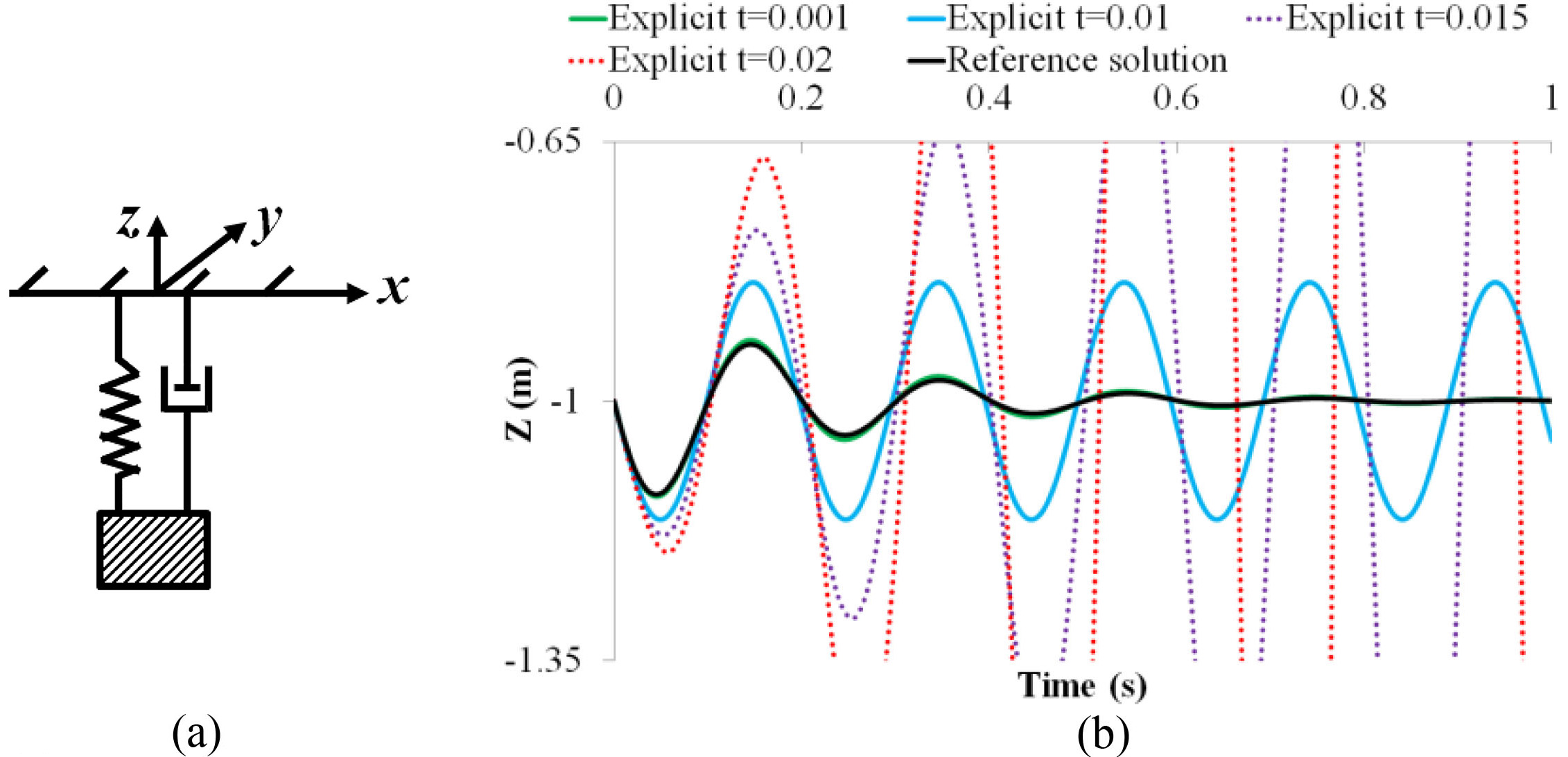
Figure 2.

(a) A comparison between the explicit integration and CNN, (b) solutions of the CNN remain stable at a large time step.

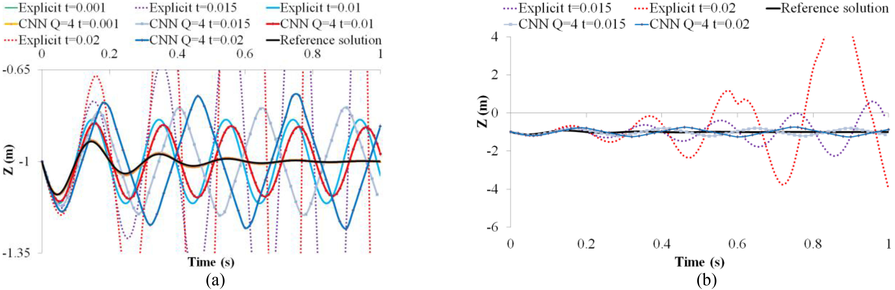
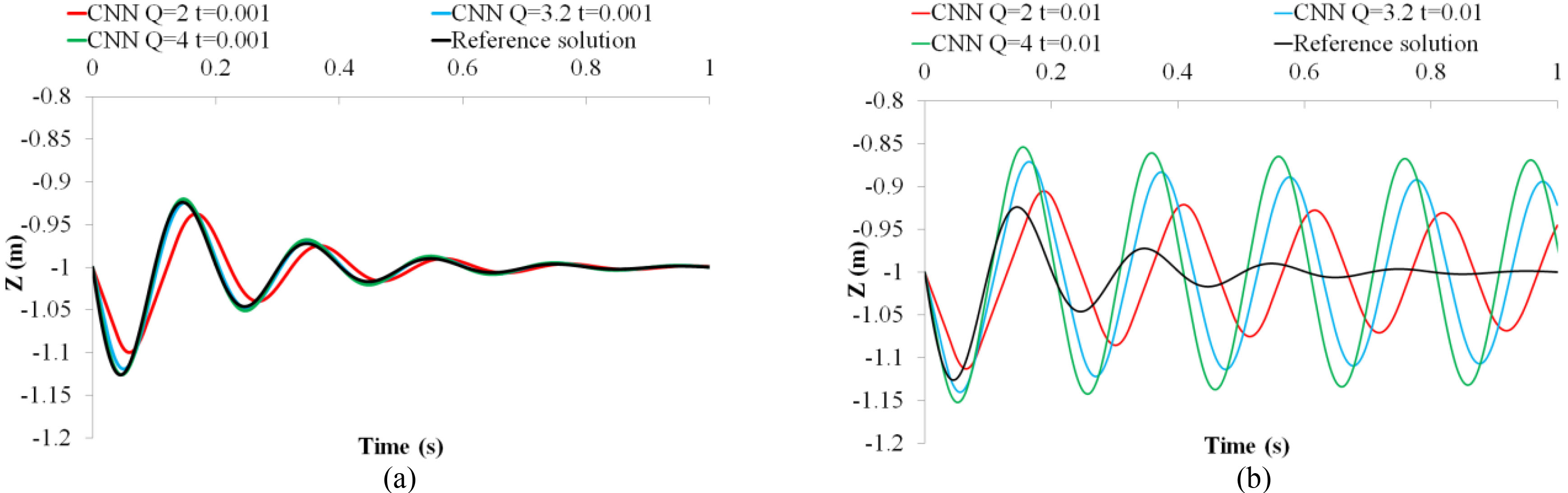
With the above same time steps, the CNN solutions shown in Fig. 2a are better than those of the explicit integration. At a small time step (e.g., t= 0.001), the CNN solution is almost identical to the reference solution. At a large time step (e.g., t= 0.015 and t= 0.02), unlike the unstable behaviour of the explicit integration, the CNN solution remains stable. A more clear illustration can be seen from Fig. 2b, which demonstrates that the CNN solution is stable whereas the solution of the explicit integration is divergent at a large time step.

Trials with three different values of Q have also been conducted to examine the effect of Q on the CNN solution. As illustrated in Fig. 3a, the CNN solutions are converged for various values of Q at a small time step and they all have a good approximation to the reference solution. Among them, the CNN solutions with Q= 4 and Q= 3.2 are the best. This is because the cell states vx⁢(t) are always in the region d⁢f⁢(v𝑥𝑖𝑗)/d⁢v𝑥𝑖𝑗=1 of the nonlinear controlled source. With a smaller value of Q= 2, the cell states vx⁢(t) could fall into the region d⁢f⁢(v𝑥𝑖𝑗)/d⁢v𝑥𝑖𝑗=0 of the nonlinear controlled source, resulted in a damped velocity for displacement calculation. Hence, the results are affected at a small time step with a smaller displacement than the reference solution (red line in Fig. 3a). However, as shown in Fig. 3b, at a large time step, the smaller the value of Q is, the better the CNN solution is, and thus the better the soft tissue deformation is. The above demonstrates that the value of Q controls the maximum displacement at each time step, and a smaller value of Q is preferred to ensure the accuracy while maintaining the stability at a large time step.

Figure 3.

Comparisons between different values of Q in the proposed CNN at (a) a small time step and (b) a large time step.

4.2Soft tissue deformation

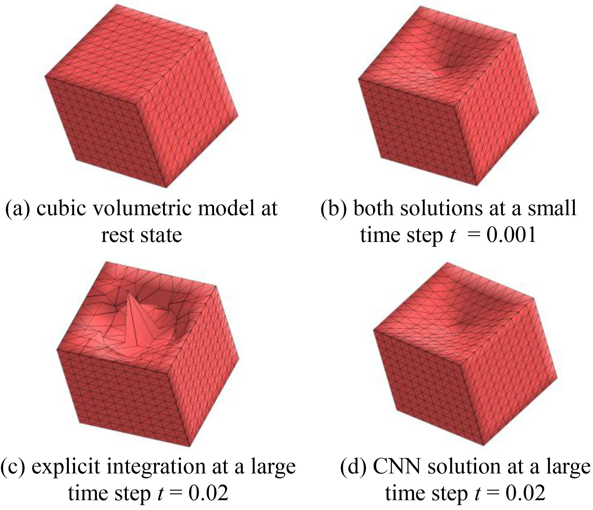
Trials have also been conducted on a cubic volumetric model of 1331 mass points and 6000 tetrahedrons, with side faces fixed (Fig. 4a) subjected to an applied force on the top surface in the normal direction, to evaluate the performance of the proposed CNN in terms of simulating soft tissue deformation. The mass matrix 𝑴, damping matrix 𝑫 and stiffness matrix 𝑲 were initialized according to the formulation proposed by Duan et al. [20], where the mass density ρ and Young’s modules E were set to 1,060 kg/m3 [21] and 3.5 kPa [22] of the soft tissue material properties. Both CNN and explicit integration were conducted under the same conditions with Q= 4 used in the CNN. As shown in Fig. 4b, both methods yield identical results at the small time step t= 0.001. However, as shown in Fig. 4c, the solution of the explicit integration become unstable at the large time step t= 0.02 whereas the CNN solution remains stable in Fig. 4d. This demonstrates that the CNN not only inherits the accuracy of the explicit integration at small time steps but also overcomes the unstable problem of the explicit integration at large time steps. It should be mentioned that the computational time of one iteration for both CNN and explicit integration are similar which is around 2 ms.

Figure 4.

Comparison between the proposed CNN and explicit integration at a small and large time step.

5.Conclusion

This paper presents a cellular neural network method for stable simulation of soft tissue deformation for surgical simulation. This method models the dynamic behaviours of soft tissues via the nonlinear neural dynamics of CNN by formulating the local connectivity of cells as the discrete non-rigid motion equation. Experimental results demonstrate that the proposed method can achieve good accuracy at a small time step and still remains numerically stable at a large time step while maintaining the computational efficiency of explicit integration. Future research work will focus on the use of nonlinear strain-stress relationship to formulate the local connectivity of cells to further improve modelling realism.

Conflict of interest

None to report.

References

[1]	Miller K. Computational Biomechanics for Patient-Specific Applications. Annals of Biomedical Engineering. (2016) ; 44: (1): 1-2. doi 10.1007/s10439-015-1519-9.
[2]	Platt SM, Badler NI. Animating facial expressions. ACM SIGGRAPH Computer Graphics. (1981) ; 15: (3): 245-52.
[3]	Terzopoulos D, Platt J, Barr A, Fleischer K. Elastically deformable models. ACM SIGGRAPH Computer Graphics. (1987) ; 21: (4): 205-14.
[4]	Misra S, Ramesh KT, Okamura AM. Modeling of Tool-Tissue Interactions for Computer-Based Surgical Simulation: A Literature Review. Presence: Teleoperators and Virtual Environments. (2008) ; 17: (5): 463-91. doi 10.1162/pres.17.5.463.
[5]	Hauth M, Etzmu O, Stra W. Analysis of numerical methods for the simulation of deformable models. The Visual Computer. (2003) ; 19: (7-8): 581-600. doi 10.1007/s00371-003-0206-2.
[6]	Cotin S, Delingette H, Ayache N. A hybrid elastic model for real-time cutting, deformations, and force feedback for surgery training and simulation. The Visual Computer. (2000) ; 16: (8): 437-52. doi 10.1007/Pl00007215.
[7]	Goulette F, Chen Z-W. Fast computation of soft tissue deformations in real-time simulation with Hyper-Elastic Mass Links. Computer Methods in Applied Mechanics and Engineering. (2015) ; 295: : 18-38. doi 10.1016/j.cma.2015.06.015.
[8]	Liu T, Bargteil AW, O’Brien JF, Kavan L. Fast simulation of mass-spring systems. ACM Transactions on Graphics (TOG). (2013) ; 32: (6): 214. doi 10.1145/2508363.2508406.
[9]	Courtecuisse H, Allard J, Kerfriden P, Bordas SPA, Cotin S, Duriez C. Real-time simulation of contact and cutting of heterogeneous soft-tissues. Medical Image Analysis. (2014) ; 18: (2): 394-410. doi 10.1016/j.media.2013.11.001.
[10]	Meier U, Lopez O, Monserrat C, Juan MC, Alcaniz M. Real-time deformable models for surgery simulation: a survey. Computer Methods and Programs in Biomedicine. (2005) ; 77: (3): 183-97. doi 10.1016/j.cmpb.2004.11.002.
[11]	Szolgay P, Vörös G, Eröss G. On the applications of the cellular neural network paradigm in mechanical vibrating systems. IEEE Transactions on Circuits and Systems I: Fundamental Theory and Applications. (1993) ; 40: (3): 222-7. doi 10.1109/81.222805.
[12]	Zhong Y, Shirinzadeh B, Alici G, Smith J. A Cellular Neural Network Methodology for Deformable Object Simulation. IEEE Transactions on Information Technology in Biomedicine. (2006) ; 10: (4): 749-62. doi 10.1109/TITB.2006.875679.
[13]	Zhong Y, Shirinzadeh B, Smith J. Soft tissue deformation with neural dynamics for surgery simulation. International Journal of Robotics and Automation. (2007) ; 22: (1): 1-9. doi 10.2316/Journal.206.2007.1.206-1000.
[14]	Fung Y-C. Biomechanics: Mechanical Properties of Living Tissues. ed n, editor: Springer-Verlag; (1993) .
[15]	Maurel W, Wu Y, Thalmann NM, Thalmann D. Biomechanical models for soft tissue simulation: Springer; (1998) .
[16]	Chua LO, Yang L. Cellular Neural Networks: Theory. IEEE T Circuits Syst. (1988) ; 35: (10): 1257-72. doi 10.1109/31.7600.
[17]	Thiran P, Setti G, Hasler M. An Approach to Information Propagation in 1-D Cellular Neural Networks – Part I: Local Diffusion. IEEE Transactions on Circuits and Systems I: Fundamental Theory and Applications. (1998) ; 45: (8): 777-89. doi 10.1109/81.704819.
[18]	Setti G, Thiran P, Serpico C. An Approach to Information Propagation in 1-D Cellular Neural Networks – Part II: Global Propagation. IEEE Transactions on Circuits and Systems I: Fundamental Theory and Applications. (1998) ; 45: (8): 790-811. doi 10.1109/81.704820.
[19]	Roska T, Chua LO. Cellular neural networks with non-linear and delay-type template elements and non-uniform grids. International Journal of Circuit Theory and Applications. (1992) ; 20: (5): 469-81.
[20]	Duan Y, Huang W, Chang H, Chen W, Zhou J, Teo SK, et al. Volume Preserved Mass-Spring Model with Novel Constraints for Soft Tissue Deformation. IEEE Journal of Biomedical and Health Informatics. (2016) ; 20: (1): 268-80. doi 10.1109/JBHI.2014.2370059.
[21]	Barauskas R, Gulbinas A, Barauskas G. Investigation of radiofrequency ablation process in liver tissue by finite element modeling and experiment. Medicina. (2007) ; 43: (4): 310-25.
[22]	Peterlík I, Duriez C, Cotin S. Modeling and real-time simulation of a vascularized liver tissue. Medical Image Computing and Computer-Assisted Intervention-MICCAI 2012: Springer; (2012) . p. 50-7.