
Using machine learning algorithms to identify farms on the 2022 Census of Agriculture1
Abstract
As is the case for many National Statistics Institutes, the United States Department of Agriculture’s (USDA’s) National Agricultural Statistics Service (NASS) has observed dwindling survey response rates, and the requests for more information at finer temporal and spatial scales have led to increased response burdens. Non-survey data are becoming increasingly abundant and accessible. Consequently, NASS is exploring the potential to complete some or all of a survey record using non-survey data, which would reduce respondent burden and potentially lead to increased response rates. In this paper, the focus is on a large set of records associated with potential farms, which are operations with undetermined farm status (farm/non-farm) and are referred to here as operations with unknown status (OUS). Although they usually have some agriculture, most OUS records are eventually classified as non-farms. Those OUS that are classified as farms tend to have higher proportions of producers from under-represented groups compared to other records. Determining the probability that an OUS record is a farm is an important step in the imputation process. The OUS records that responded to the 2017 U.S. Census of Agriculture were used to develop models to predict farm status using multiple data sources. Evaluated models include bootstrap random forest (RF), logistic regression (LR), neural network (NN), and support vector machine (SVM). Although the SVM had the best outcomes for three of the five metrics, the sensitivity for identifying farms was the lowest (13.8%). The NN model had a sensitivity of 80.5%, which was substantially higher than the other models, and its specificity of 45.3% was the lowest of all models. Because sensitivity was the primary metric of interest and the NN performed reasonably well on the other metrics, the NN was selected as the preferred model.
1.Introduction
The United States Department of Agriculture’s (USDA’s) National Agricultural Statistics Service(NASS) conducts more than 100 surveys each year, producing more than 400 agricultural reports annually, and the Census of Agriculture (Census) every 5 years. These reports are utilized for a variety of applications, from public policy decisions to price estimates and research. The published data are under strict confidentiality constraints. This requires that published granular-level estimates (particularly at the county level) include enough producers in that area such that data can be aggregated to protect confidentiality. This becomes more challenging as the demand for information at finer temporal and spatial scales increases. At the same time, many survey areas, including agriculture, have observed a steady decline in response rates over recent years [1, 2]. To conduct most surveys and the Census, NASS uses a list frame, a comprehensive list of all known and potential farms in the U.S. A farm is defined as a place from which $1,000 or more of agricultural products were produced and sold, or normally would have been sold, during the year, including any government agricultural payments received. The list frame is updated regularly to maintain current information on each record and serves as the foundation for the development of the Census Mail List.
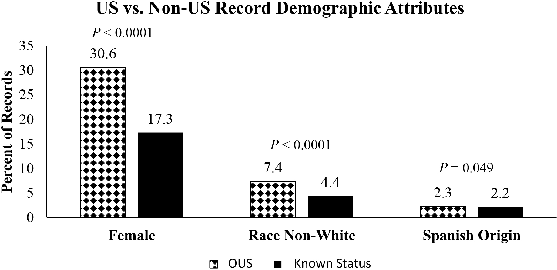
Figure 1.
Demographic characteristics of primary producers identified in farm and non-farm records in the 2017 U.S. Census of Agriculture.
NASS builds and improves the list frame on an ongoing basis. Lists are obtained from multiple sources, including state and federal government agencies, producer associations, and marketing associations. NASS also obtains special commodity lists to address specific deficiencies. These outside source lists are matched to the NASS list frame using record linkage. Most of the records obtained are already on the NASS list frame; however, any record not currently on the frame is classified as a potential farm until NASS can confirm whether the associated operation meets the definition of a farm.
Each operation on the list frame is assigned an active status (AS) code to classify the record as an active, potential, or inactive farm. Active records represent operations that have been confirmed to be farms and are thus assumed to have a high probability of representing active farming operations. Potential farms are those operations identified during the list building process as being associated with agriculture, but their farm status has not been assessed and is thus unknown. Inactive records may be associated with landlords, deceased producers, farms no longer in business, etc. Some active records represent agricultural establishments that operate land but do not have sufficient production to be classified as a farm in a specific year. These are maintained on the list frame as active records to help ensure high coverage of farms for the Census every five years.
Potential farms are periodically screened to determine whether they satisfy the definition of a farm. In this effort, NASS conducts the National Agricultural Classification Survey (NACS) each year. This survey collects data from potential farms to establish whether they meet the definition of a farm. The status code of each responding record is changed to indicate the operation is either a farm or a non-farm. The subset of potential farm records that have not responded to any NACS and thus have unknown farm status are classified as operations with unknown status (OUS) for the current Census.
For the 2017 U.S. Census of Agriculture, 356,889 (12%) of the records on the Census list frame were OUS records. Of these, 74,040 (22%) responded to the Census and, of those responding, 20,414 (26%) were farms. In comparison, the overall response rate for the 2017 Census, which included the OUS, was 72%. With the low response rates and the small proportion of responding OUS records that are farms, OUS data collection costs tend to be high. However, the OUS records identified as farms during the Census had significantly higher proportions of producers from under-represented groups, including female producers and producers of Hispanic and non-white origin (Fig. 1). Obtaining responses from as many of these records as possible would improve overall response rates, increase representativeness, may lead to more precise estimates, and could increase the number of published county-level estimates.
Figure 2.
Map of the proportion of 2017 U.S. Census of Agriculture records that were OUS.
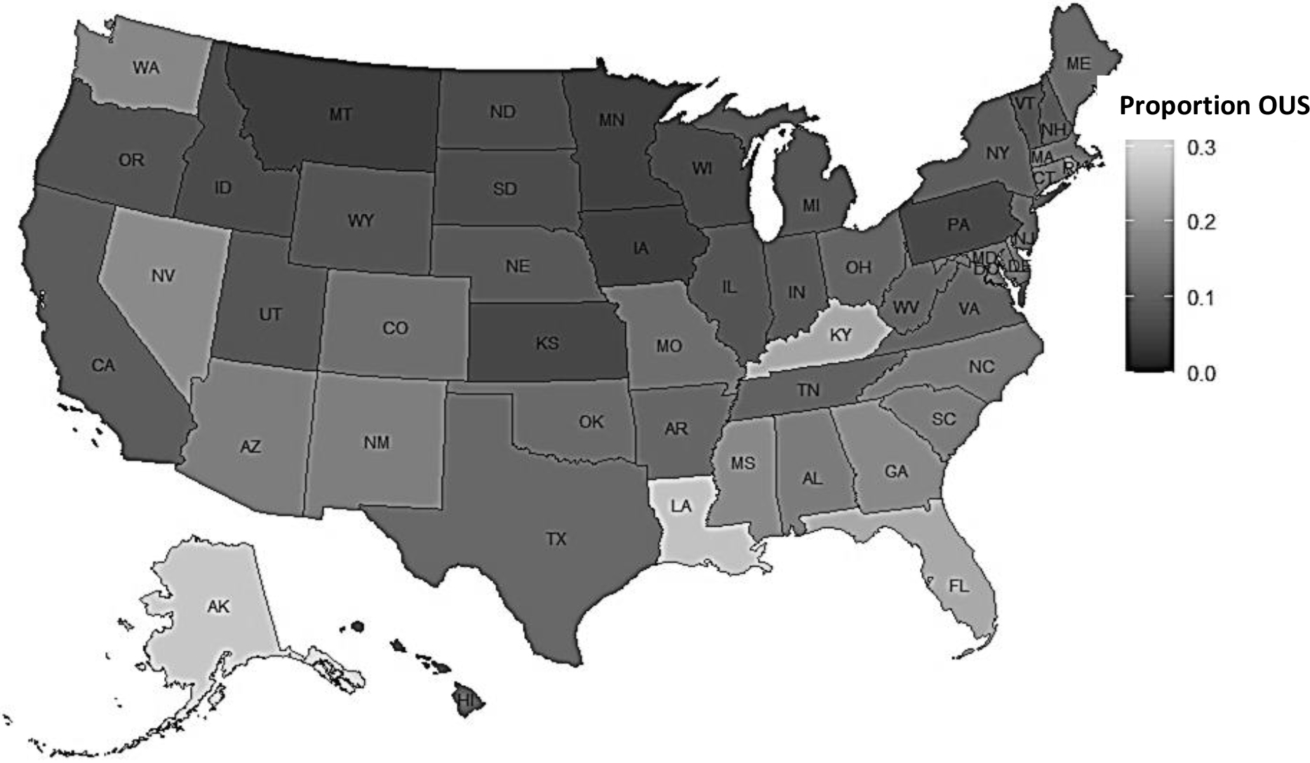
Figure 3.
Map of the proportion of 2017 U.S. Census of Agriculture OUS records that responded.
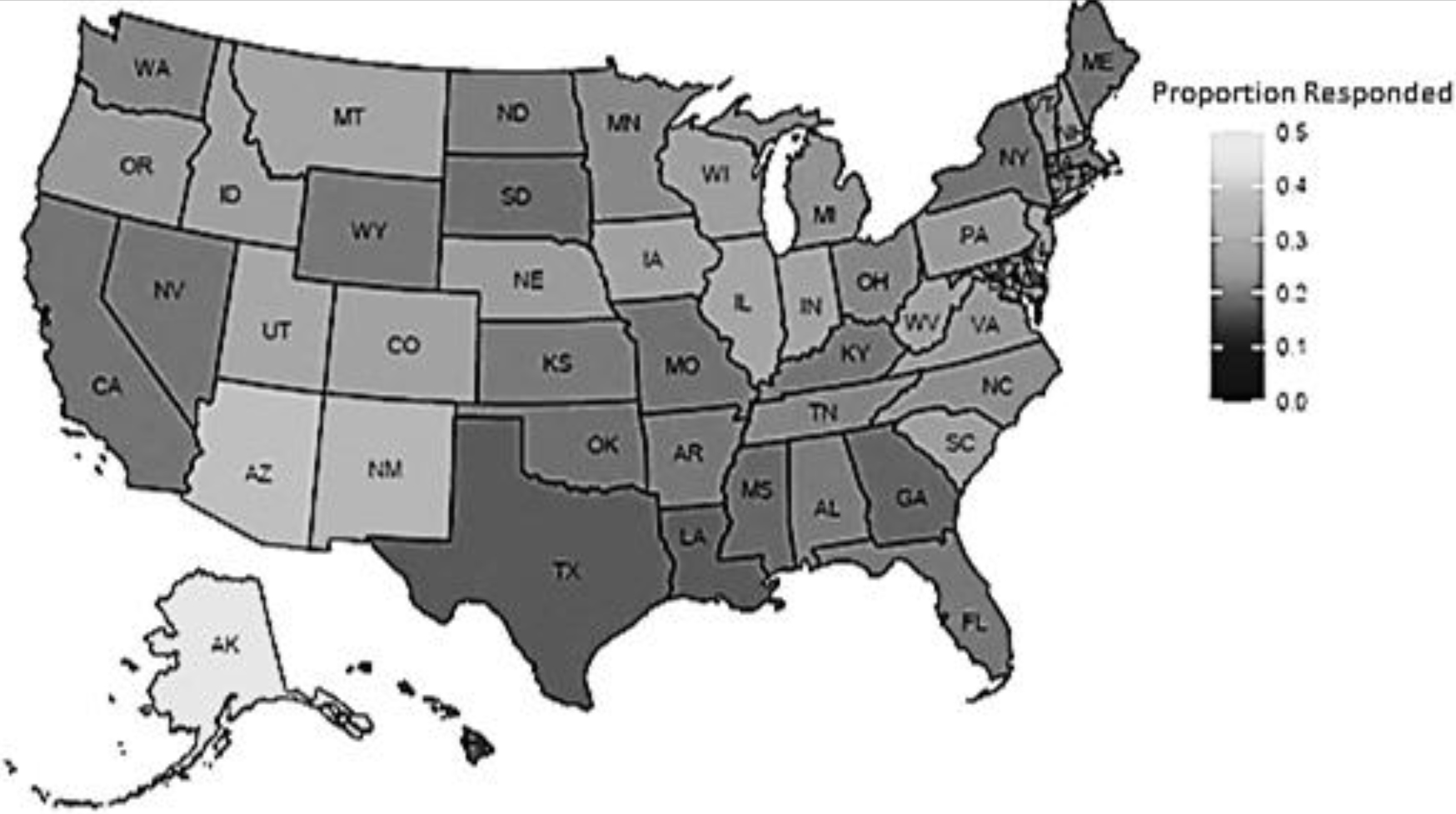
Figure 4.
Map of the proportion of responding 2017 U.S. Census of Agriculture OUS records that were farms.
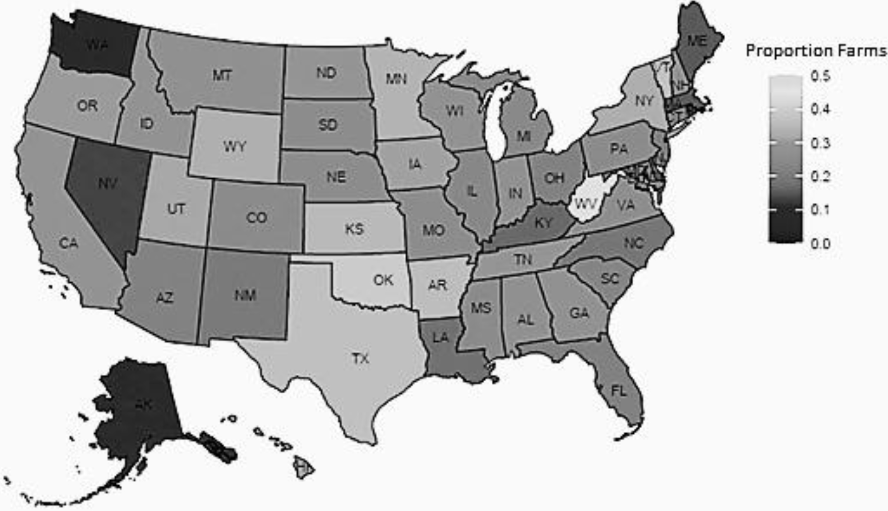
The proportion of Census OUS records varies by state, exceeding 30% in some states (see Fig. 2). The Census response rates of OUS records and the proportion of responding OUS records that are farms vary by state (see Figs 3 and 4). Using 2022 administrative and other non-survey data to complete the OUS records would provide richer information for estimation while potentially reducing respondent burden and costs. Because not all OUS records are farms, an important first step is to estimate the probability of an OUS record being a farm based on its characteristics. In this work, it is assumed that records with the same characteristics have the same probability of being a farm, whether they responded or did not respond to the Census. How these probabilities of records being a farm could be used in the estimation process will be discussed in the last section.
The USDA NASS uses various types of machine learning to analyze agricultural data and derive meaningful insights. NASS may use supervised learning algorithms to forecast crop yields based on historical data, weather patterns, and other relevant factors. Unsupervised learning algorithms are also utilized by NASS to identify patterns and structures within agricultural datasets without explicit labeling. Clustering algorithms, such as K-means clustering, help NASS group similar data points together, aiding in the identification of trends or anomalies in agricultural production or land use patterns. Additionally, NASS leverages ensemble methods, such as random forests and gradient boosting, to generate propensity scores for more efficient data collection. NASS explores emerging techniques, such as deep learning and natural language processing, to extract insights from unstructured data sources, such as satellite imagery and textual reports. Deep learning algorithms, including convolutional neural networks (CNNs) and recurrent neural networks (RNNs), enable NASS to analyze complex spatial and temporal patterns in agricultural data, facilitating more comprehensive assessments of crops, land use changes, and environmental impacts. See [3, 4, 5] for a detailed overview of current and past data sources and statistical techniques.
A few notable applications of machine-learning within NASS include:
1. Crop Yield Prediction: Numerous studies have focused on using machine learning algorithms to predict crop yields based on various factors such as historical yield data, weather patterns, soil characteristics, and crop management practices. The aim is often to improve the accuracy and reliability of crop yield forecasts, aiding farmers, policymakers, and other stakeholders in decision-making processes [4, 6, 7].
2. Land Use Classification: Machine learning techniques, including supervised and unsupervised learning algorithms, have been applied to satellite imagery and other remote sensing data to classify land use and land cover types. These studies help monitor changes in agricultural landscapes, assess the impacts of land management practices, and inform land-use planning initiatives [8].
3. Survey Methodology Optimization: USDA NASS conducts numerous surveys to collect agricultural data from farmers and other stakeholders. Machine learning algorithms have been utilized to optimize survey methodologies, including sample design, questionnaire design, and data collection strategies, to improve the efficiency and accuracy of data collection processes [9, 10].
Here the study objective is to utilize the responses from OUS records in the 2017 U.S. Census of Agriculture to develop a model that can be used to predict whether an OUS record meets the farm definition. The study was initiated to inform data collection and potential imputation for the 2022 Census. Thus, the time and resources available for the study were limited.
In the next section, a detailed overview of the approach used in this study to predict which OUS records are farms. The dataset composition, candidate model specifications, and model comparison techniques are described.
2.Methodology
Data used in this study were the 74,040 OUS records that responded to the 2017 Census. Of these, 17,766 were classified as farms. The data were divided into training (70%; 51,828 records) and testing (30%, 22,212 records) sets with equal proportions of farm and non-farm records as suggested by Vrigazova [11]. In a set of simulation studies using real data, Vrigazova [11] found that splitting the dataset with the 70/30 train/test proportion usually provides the most accurate results. Agricultural variables were omitted from modeling for two reasons: 1) the extremely sparse reporting of agricultural information by the OUS farms in the 2017 Census data; and 2) with rare exceptions, the 2022 OUSs did not have agricultural data as these were still operations that had not reported to NASS. Furthermore, linkage between the OUS records and the NASS area frame, which covers the conterminous U.S., is not a viable option because the OUSs were not geospatially linked to the area frame, which is needed to acquire the information.
Variables available for analysis were:
• Year the record was linked to the list frame.
• Source of the record.
• Geospatial information: state, county, district, 5-digit zip code, 4-digit zip code extension, and full geographic variable (combination of these variables) for the operation location.
• Last date the record was considered active.
• Demographic information: race (white or non-white), whether the producer was of Spanish or Hispanic origin (yes, no, or unknown), age category (
• Indicator variables for whether the record included a producer or other phone number, with values of 1 indicating the presence of a phone number and 0 indicating no phone number.
• Indicator variable for whether the record was flagged as a high impact record, with a value of 0 indicating a normal record and a value of 1 indicating a record that required data collection or imputation (in cases of refusal or inaccessibility to a respondent) due to its expected impact on specific commodity (commodities).
Responding OUS records to the 2017 Census do have some agricultural data, but all records need to have this information for them to be useful in the modeling process.
Table 1
Model specifications for the random forest model
| Specification | |
| Trees | 42 |
| Rondom split points (node) | 10 |
| Bootstrap protocol | WR |
| Impute iterations | 2 |
| Weights | Yes |
Machine learning models were developed to predict OUS farm status using R and python. The bootstrap random forest (RF) was trained and tested in the R randomForestSRC-package [12] with specifications shown in Table 1. Logistic regression (LR) was conducted in R using the function glm() from the package stats, which uses the Fisher scoring algorithm [4]. Neural network (NN) and support vector machine (SVM) were trained and tested in python. In particular, the NN was implemented using the keras API provided by the tensorflow package [13, 14, 15, 16, 17], and the implementation of Support Vector Classifiers (SVCs) available from the scikit-learn package was used for the SVM. Furthermore, all four models were trained using weights. These weights were included to cope with unbalanced data by adjusting for the proportion of records classified as farms vs. non-farms.
The SVM model was trained using the default settings of the SVM algorithm in the scikit-learn package. That is, the regularization parameter was set to one, and the kernel was formulated as a radial basis function with scale parameter equal to , where denotes the number of variables. In general, the approach proposed by [18] is adopted to compute probabilities for multi-class classification problems. However, the probabilities from the binary SVC in this paper were calibrated using Platt’s scaling method [19], which uses 5-fold cross-validation on the training data to fit logistic regressions on the SVM scores. Because the classification probabilities were calibrated, the outputs of the SVC were in the interval [0, 1].
Table 2
Structure of the neural network used for identifying farms with active status
| Layer type | Output neurons | Processed information received from layer |
|---|---|---|
| Input Layer | 18 | |
| Dropout at 25% | 18 | 1. |
| Dense with linear activation | 32 | 2. |
| Dense with rectified linear units | 32 | 2. |
| Multiply (i.e., concatenate with interactions) | 1088 | (3., 4.) |
| Dropout at 50% | 1088 | 5. |
| Dense with rectified linear units | 4 | 6. |
| Dense with rectified linear units | 4 | 3. |
| Multiply (i.e., concatenate with interactions) | 24 | (7., 8.) |
| Dropout at 5% | 24 | 9. |
| Dense with sigmoidal activation (in output) | 1 | 10. |
Table 3
Variable importance computed using the weight values from the neural network
| Variables | Importance |
|---|---|
| Year record added to the list frame | 2.49 |
| Source of record | 2.49 |
| Indicator of whether the record is expected to have a major impact on a commodity’s estimate | 2.21 |
| State | 2.16 |
| Sex of the producer | 2.15 |
| Indicator that the primary producer is Hispanic | 2.07 |
| Primary producer’s age category | 2.03 |
| Agricultural district | 2.02 |
| County of the operation | 2.01 |
| Date last active | 2.01 |
| Other phone number indicator | 1.99 |
| Phone number indicator | 1.94 |
| Producer race | 1.91 |
The NN model was designed to account for interaction between pairs of hidden layers. See Table 2 for more information about the architecture of the network. The training of the NN model was performed by minimizing the binary cross entropy loss function with the RMSprop optimization algorithm [20]. Because this algorithm is based on the concept of stochastic gradient descent, the records were randomly assigned to their respective mini batches. Using default values, the size of the mini batches was kept at 32 samples; a single epoch was performed; and the optimization method used a learning rate of 0.001, a discounting factor of 0.9, and zero momentum. Because the sigmoidal activation function was used as the output layer in the NN model, the resulting probabilities were in the interval [0, 1]. Due to memory constraints, the ZIP-code indicator variables were not used in the NN.
Table 4
Model evaluation metrics for model performance in predicting farm status of records in the testing data set
| Metric | RF | SVM | NN | LR |
|---|---|---|---|---|
| Accuracy1 | 67.26% | 72.90% | 53.80% | 66.40% |
| Sensitivity2 | 66.75% | 13.80% | 80.50% | 67.30% |
| Specificity3 | 67.42% | 96.40% | 45.30% | 66.20% |
| Precision4 | 27.05% | 54.30% | 31.70% | 38.60% |
| AUC5 | 72.63% | 72.50% | 72.10% | 71.80% |
1Accuracy
Using the validation data, all models were evaluated for accuracy, sensitivity, specificity, and area under the receiver-operating characteristic curve (AU-ROC). In the context of this study, accuracy is defined as the proportion of records that were correctly classified by the model (correctly identified as a farm or as a non-farm). Sensitivity is the proportion of farms that were correctly classified by the model. Specificity is the proportion of non-farms that were correctly classified by the model. The AUC is the area under the Receiver Operating Curve (ROC), which is a plot of the sensitivity versus (1 – specificity). The AUC can be between 0.5 and 1.0, with higher values indicating a better model. Model comparisons were based on all metrics; however, sensitivity was considered the most important model outcome. In the Census, further record evaluation and imputation processes may remove records as non-farms after this initial classification, so misclassifying a record as a farm was considered less important than potentially missing records that were farms.
3.Results
All models included all variables. For the LR model, all variables were significant (
The overall accuracy of a classification approach based on the majority class observed in the training set (i.e., classifying all records as non-farms) was 76% for the validation set, which is greater than that of any of the fitted models (see Table 4). However, the sensitivity and specificity in the validation set were 0% and 100%, respectively. The four fitted models have much higher sensitivity at the cost of a lower specificity. Therefore, the four fitted models provide a higher applicate value for the correct identification of farm status among the true farms within OUS records. Conversely, assuming a classification approach based on the minority farm, the results from the validation data would have been a 23% overall accuracy, 100% sensitivity, and 0% specificity. However, this approach could result in a large percentage (
SVM had the best outcomes for three of the evaluation metrics (accuracy, sensitivity, and specificity, see Table 4). The RF and LR models produced comparable results in accuracy, sensitivity, and specificity, and the precision of the RF model (27.05%) was below that of the LR model (38.6%). The NN produced the highest sensitivity (80.5%), and the SVM had the smallest (13.8%). These values indicate that the NN was much better able to identify true farms. The cost of these positive identifications was lower specificity of the NN (45.3%) compared to the SVM (96.4%). Given that sensitivity was identified as the most important metric and the specificity is still reasonable, the NN was identified as the best model.
4.Discussion
The U.S. has a de-centralized Federal Statistical System (FSS). The laws governing the protection of respondents’ data are usually specific to each agency within the USFSS. As examples, Title 7 governs how NASS is to protect the data it collects whereas Title 13 determines the confidentiality constraints of the U.S. Census Bureau. Thus, gaining access to administrative and other non-survey data for imputation is more complex than in numerous other countries. Yet, increasingly, agencies within the FSS are working across agency boundaries in their efforts to explore opportunities to decrease or eliminate respondent burden by using diverse data sources to obtain the information needed to produce official statistics.
NASS has begun identifying data sources that can be used to complete some or all of the responses for its 2027 U.S. Census of Agriculture. The OUS project described here is an initial step in that direction. Modeling the probability of an OUS record meeting the definition of a farm, and the extension to other records on the NASS list frame, has application beyond the Census. Costs may be reduced by incorporating the probability of a record representing a farm into the data collection process. Sample selection could be informed by this probability, and the number of contact attempts could also vary with the probability of the operation being a farm.
In all models, it was assumed that the probability of an OUS record is associated with a farm is the same whether the producer responded to the Census. Assessing the validity of the assumption is a major challenge as most nonresponding OUS records have been contacted numerous times without obtaining a response. One approach may be to evaluate the proportion of responding OUS records that are found to be farms after each contact. Recall that once an OUS responds the operation is classified as a farm/nonfarm and is no longer an OUS. If the proportion classified as farms is the same after the first, second, and subsequent contacts, then the assumption is more likely to be valid than if the proportion of farms decreases (or increases) with each contact. If the rate of decrease can be quantified, perhaps an adjustment for nonresponse bias can be developed. This is an area for future research.
For this application, it was decided to identify those records most likely to be farms and to impute only for those records. The alternative was to weight each record by its probability of being a farm. Because OUSs are a rich source of information on under-represented groups, this approach could lead to imputing records for these groups in counties without any producers in that group. For example, an estimate of the number of Asian female producers could be provided for a county without any producers in this demographic group. Whether this would have been an issue needs to be further studied. Because the proportion of OUS records representing farms is small, failing to either classify records as being farms or non-farms or adjust a record’s weight by the probability of it being a farm, would lead to an upward bias in the estimated total number of OUS farms. The uncertainties associated with estimating the probabilities and the subsequent classification of records as farms and non-farms should be reflected in the uncertainties of the subsequent population estimates. How best to do that is another area of potential research.
These models could be modified or re-evaluated for improvement. As artificial intelligence (AI) and other data science methods become available, the choices of data and potential models are growing, and the probability of a record being associated with a farm will become more precise. In addition, the models should be generalized for repeated use over time. As an example, as one referee noted, recasting the time related variables of “Year” and “Time Since Last Active” as values relative to a meaningful reference point could ensure temporal validity when applying the models in later years.
With the current approach, the probability cutoffs for classifying a record as a farm could be modified to favor sensitivity or specificity, depending on the importance of misclassification type. Over-predicting records as farms would increase the number of actual farms detected and reduce the risk of not including these records. However, it would also increase the number of non-farms included, which could reduce estimation accuracy or increase cost. This balance should be carefully considered for final model determination.
Future model evaluation should also include a comparison of misclassification rates. Accurate representation of minority producers (e.g., female and/or non-white) is an important goal for the USDA. To determine any model bias associate with any specific group, the misclassification rates across all demographic groups of producers should be evaluated and, if needed, model adjustments should be made to eliminate bias.
The distribution of OUS records and the proportion meeting the definition of a farm may differ across Census cycles. Utilizing past Census data to predict the status of future records may not be sufficient. If this is the case, the models may only be applicable for post-data collection imputation, using the current OUS responses for model development. If the models are accurate across Census cycles, they could be used before survey administration to inform mailing and nonresponse follow-up.
Because the OUS records have never responded to any NASS survey, the amount of information and variables available for modeling these records is minimal. Identifying additional potential sources, such as administrative and web-scraped data, may lead to additional, useful information for the modeling efforts.
Acknowledgments
We would like to extend our sincere appreciation to the two reviewers for their valuable comments and suggestions, which have improved the quality of this paper. Their insightful feedback has been instrumental in refining our work. The findings and conclusions in this article are those of the authors and should not be construed to represent any agency determination or policy. They have not been formally disseminated by the U.S. Department of Agriculture.
References
[1] | Stedman RC, Connelly NA, Heberlein TA, Decker DJ, Allred SB. The end of the (research) world as we know it? Understanding and coping with declining response rates to mail surveys. Society & Natural Resources. (2019) Oct; 32: (10): 1139-54. |
[2] | Johansson R, Effland A, Coble K. Falling response rates to USDA crop surveys: Why it matters. Farmdoc Daily. (2017) Jan 19; 7: (9). |
[3] | Johnson DM. An assessment of pre-and within-season remotely sensed variables for forecasting corn and soybean yields in the United States. Remote Sensing of Environment. (2014) Feb 5; 141116-28. |
[4] | Young LJ. Agricultural crop forecasting for large geographical areas. Annual Review of Statistics and Its Application. (2019) Mar 7; 6: : 173-96. |
[5] | Di Paola A, Valentini R, Santini M. An overview of available crop growth and yield models for studies and assessments in agriculture. Journal of the Science of Food and Agriculture. (2016) Feb; 96: (3): 709-14. |
[6] | Zhang C, Yang Z, Di L, Lin L, Hao P, Guo L. Applying machine learning to cropland data layer for agro-geoinformation discovery. In: 2021 IEEE International Geoscience and Remote Sensing Symposium. IGARSS; (2021) Jul 11; pp. 1149-52. |
[7] | Zhang C, Marfatia P, Farhan H, Di L, Lin L, Zhao H, Li H, Islam MD, Yang Z. Enhancing USDA NASS cropland data layer with segment anything model. In: 11th International Conference on Agro-Geoinformatics. Agro-Geoinformatics; (2023) Jul 25; pp. 1-5. |
[8] | Hunt KA, Abernethy J, Beeson P, Bowman M, Wallander S, Williams R. Crop Sequence Boundaries (CSB): Delineated Fields Using Remotely Sensed Crop Rotations. USDA-NASS; (2023) ; Available from: https//www.nass.usda.gov/Research_and_Science/Crop-Sequence-Boundaries/index.ph. |
[9] | Sartore L, Boryan C, Dau A, Willis P. An Assessment of Crop-Specific Land Cover Predictions Using High-Order Markov Chains and Deep Neural Networks. Journal of Data Science. (2023) ; 21: (2). |
[10] | Mitchell M, Ott K, McCarthy J. Using Nonresponse Propensity Scores to Set Data Collection Procedures for the Quarterly Agricultural Survey. (2014) . |
[11] | Vrigazova B. The proportion for splitting data into training and test set for the bootstrap in classification problems. Business Systems Research: International Journal of the Society for Advancing Innovation and Research in Economy. (2021) ; 12: (1): 228-42. |
[12] | Ishwaran H, Kogalur U. Fast Unified Random Forests for Survival, Regression, and Classification (RF-SRC). R package version 3.2.3. Available from: https//cran.r-project.org/package=randomForestSRC. 2023. |
[13] | Chollet F. Keras. [online] (2015) ; 12: (01): 2021. Available at: https://github.com/fchollet/kera. Accessed May (2024) . |
[14] | Chollet F. Keras API reference. Keras. (2022) ; Available from: https//keras.io/api. |
[15] | Gulli A, Pal S. Deep learning with Keras. Packt Publishing Ltd. (2017) Apr 26. |
[16] | Abadi M, Barham P, Chen J, Chen Z, Davis A, Dean J, Devin M, Ghemawat S, Irving G, Isard M, Kudlur M. Tensorflow: a system for large-scale machine learning. In: Proceedings of the 12th USENIX Symposium on Operating Systems Design and Implementation (OSDI 16); (2016) Nov 2; Vol. 16: , pp. 265-83. |
[17] | Longford NT. A fast scoring algorithm for maximum likelihood estimation in unbalanced mixed models with nested random effects. Biometrika. (1987) ; 74: (4): 817-27. |
[18] | Wu TF, Lin CJ, Weng R. Probability estimates for multi-class classification by pairwise coupling. Advances in Neural Information Processing Systems. (2003) ; 16. |
[19] | Platt J. Probabilistic outputs for support vector machines and comparisons to regularized likelihood methods. Advances in Large Margin Classifiers. (1999) ; 10: (3): 61-74. |
[20] | Hinton G, Srivastava N, Swersky K. Neural networks for machine learning lecture 6a overview of mini-batch gradient descent. Cited on 14.8. (2012) ; 2. |
[21] | Di Paola A, Valentini R, Santini M. An overview of available crop growth and yield models for studies and assessments in agriculture. Journal of the Science of Food and Agriculture. (2016) Feb; 96: (3): 709-14. |


