
Earth observations for official crop statistics in the context of scarcity of in-situ data
Abstract
Remote sensing offers a scalable and low cost solution for the production of large-scale crop maps, which can be used to extract relevant crop statistics. However, despite considerable advances in the new generation of satellite sensors and the advent of cloud computing, the use of remote sensing for the production of accurate crop maps and statistics remain dependant on the availability of ground truth data. Such data are necessary for the training of supervised classification algorithms and for the validation of the results. Unfortunately, in-situ data of adequate quality for producing crop statistics are seldom available in many countries.
In this paper we compare the performance of two supervised classifiers, the Random Forest (RF) and the Dynamic Time Warping (DTW), the former being a data intensive algorithm and the latter a more data frugal one, in extracting accurate crop type maps from EO and in-situ data. The two classifiers are trained several times using datasets which contain in turn an increasing number in-situ samples gathered in the Kashkadarya region of Uzbekistan in 2018. We finally compare the accuracy of the maps produced by the RF and the DTW classifiers with respect to the different number of training data used. Results show that when using only 5 and 10 training samples per each crop class, the DTW reaches a higher Overall Accuracy than the RF. Only when using five times more training samples, the RF starts to perform slightly better that the DTW. We conclude that the DTW can be used to map crop types using EO data in countries where limited in/situ data are available. We also highlight the critical importance in the choice of the location of the in-situ data and its thematic reliability for the accuracy of the final map, especially when using the DTW.
1.Introduction
FAO is implementing the EOSTAT project, which aims at building the capacity of countries in using Earth Observations (EO) and remote sensing as alternative data sources for the production of official crop statistics, under the overall objective of the modernization of the National Statistics System, an initiative lead and promoted by the UN Statistical Commission.
Remote sensing is a scalable and cost-effective way of producing national-scale cropland maps: time series of open-source satellite missions, such as Sentinel 1 and 2 operated by the European Space Agency, allow distinguishing agricultural land cover from other land cover types, due to the inherently seasonal nature of crop growth, also referred to as crop phenology. Cropland masks and crop type maps produced from remotely sensed images provide essential information to accurately monitor the spatial distribution of crops and their growth conditions, enabling national authorities to adequately plan for food commodities supply, as well as to gradually reduce the threat of food insecurity. Nationwide, crop maps are instrumental tools that provide spatially explicit information about the quantity and quality of croplands, and support socio-economic decision-making.
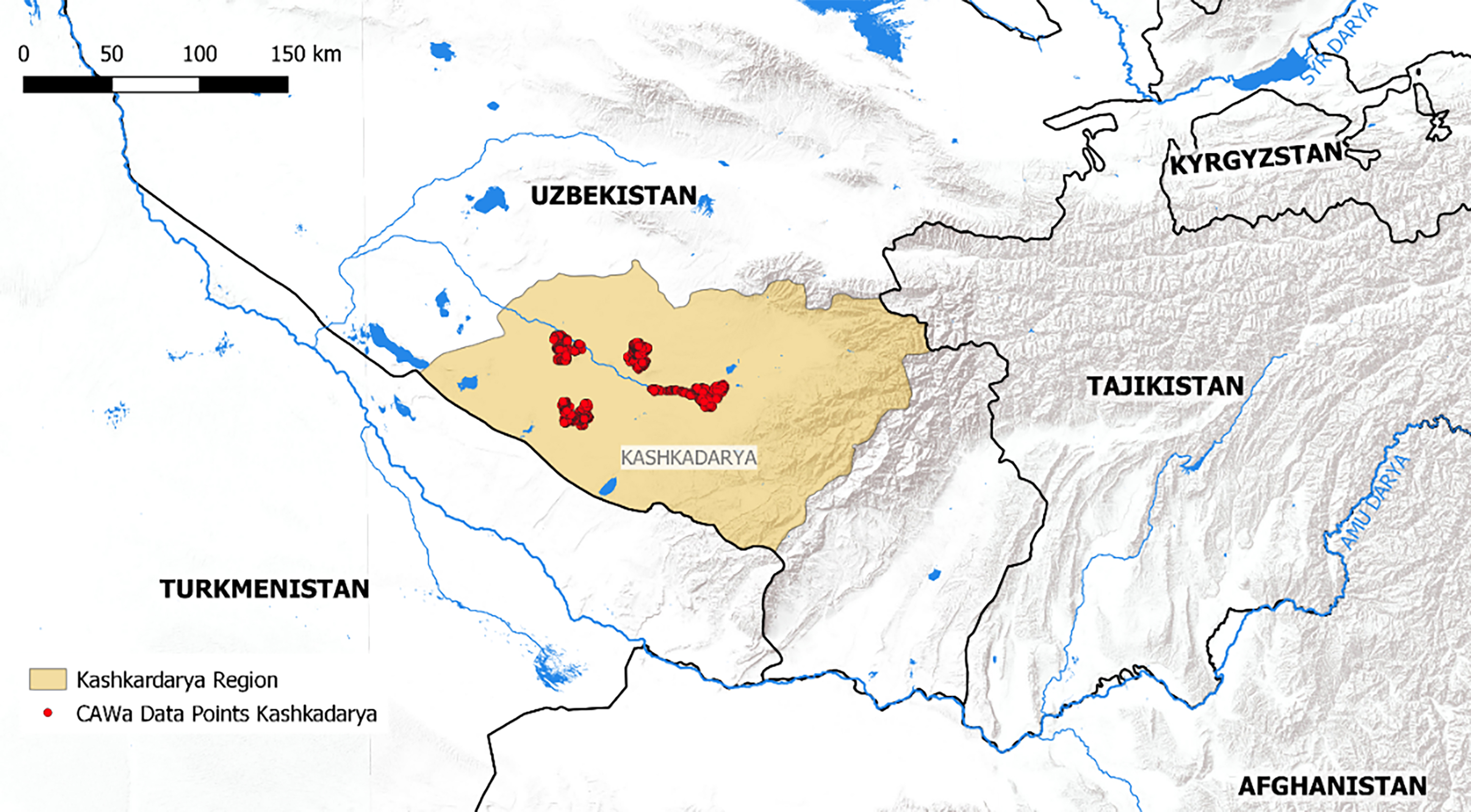
Figure 1.
Map of the main study region with the main rivers and water bodies in blue colour.
Despite the considerable advances in the new generation of satellite sensors, which provide free and open access to dense imagery time series, and the advent of cloud computing, which facilitates the storage and computation of EO data, the use of remote sensing for the production of accurate crop maps and statistics remain dependant on the availability of ground truth data. Such data, also denominated in-situ data, being collected in the field, are necessary for the training of supervised classification algorithms and for the validation of the results. However, in-situ data of adequate quality for producing crop statistics (in combination with remote sensing imageries) are seldom available in many countries, especially those with a less advanced statistical system. In-situ data are in fact either not available, or, when available, outdated and of poor quality (i.e. for suboptimal geo-referencing). In fact, crop data are often georeferenced at the farmer dwelling, rather than at the parcel level. This makes such data incompatible with the use of EO data, as it does not allow establishing a correct spatial relation between survey crop data and the pixels of the satellite image. Because of the lack of in-situ data of adequate quality, the operational uptake of EO data in NSOs is still limited. Hence, the main objective of the EOSTAT project is to promote the use of EO, also by developing and using novel classification algorithms, which may cope with scarcity of in-situ data.
In this paper, therefore, we test the performance of two supervised classifiers, the Random Forest (RF) and the Dynamic Time Warping (DTW). The former is a robust decision tree system developed by Kam Ho in 1995 [1], which performs best when trained with large in-situ data sets [2]. The latter is a data mining algorithms, and focuses on the computation of an average set of sequences and computes a dissimilarity score to compare pairs of time series data: Petitjean et al used it for the first time with satellite data in 2010 [2].
The two classifiers, which utilize Sentinel 1 and Sentinel 2 EO data, are trained several times using datasets which contain in turn an increasing number in-situ samples gathered in the Kashkadarya region of Uzbekistan (Fig. 1) in 2018. In particular, while the DTW algorithm uses respectively 5 and 10 samples, the RF algorithm employs respectively 5, 10, 20, 30, 40 and 50 training samples. We finally compare the accuracy of the maps produced by the RF and the DTW classifiers with respect to the different number of training data used.
The reference ground-truth dataset [3] has been published in Scientific Data, which is a peer-reviewed, open-access international journal for descriptions of scientifically valuable datasets. The full dataset consists of 8,196 samples collected between 2015 and 2018 in several regions of Uzbekistan and Tajikistan. In particular, 2,172 samples are available for the Kashkadarya region, where they all have been collected in the year 2018 (Fig. 1).
Table 1
Available Crop classes for Kashkadarya region, year 2018, and the respective number of geo-referenced polygons, and generated training and validation data points, respectively. The training data points for the class ‘no-crop (natural vegetation)’ were added to the dataset manually based on satellite image interpretation
| Crop class | Available polygons [N | Training data set points generated [N | Test data set points generated [N |
|---|---|---|---|
| Cotton | 945 | 50 | 892 |
| Wheat | 992 | 50 | 942 |
| Wheat–other (double cropping) | 18 | 50 | 30 |
| Alfalfa | 13 | 50 | 30 |
| Vineyards | 11 | 50 | 30 |
| Orchards | 85 | 50 | 33 |
| No-crop (fallow) | 100 | 50 | 47 |
| No-crop (natural vegetation) | – | 10 | – |
| Other | 7 | – | – |
| Total | 2172 | 360 | 2004 |
In Kashkadarya, like in the north of Afghanistan, wheat is the main staple crop. Wheat is generally harvested in June, allowing farmers to get a second harvest before the end of the agricultural season if rainfall water is available (‘double cropping’). The second most produced crop in the region is Cotton whose growing season extends from May to October. Furthermore, other important crops are orchards, vineyards, and forage crops (alfalfa).
The paper is organized as follows: Section 2.2 describes the methodology for sampling the training data and for validating the algorithms. In Section 2.2, we also illustrate the pre-processing of the EO data and we provide insights into the crop type classification algorithms, the DTW and the RF. The main results of our experiment are presented and discussed in Section 4, while in Section 2.4 we provide some concluding remarks. Classification maps and validation results can also be viewed and downloaded in the sample EOSTAT CropMapper front-end application for Kashkadarya [4].
2.Methodology
The overall methodology is articulated in four distinct steps:
1)
1. Pre-processing of the in-situ data, in order to generate subsets of training and validation samples, from the original in-situ data set.
2. Pre-processing of Sentinel 1 and Sentinel 2 data to create a harmonized time series of temporal composites.
3. Production of crop type maps using the RF and DTW classifiers.
4. Computation of accuracy measures and comparative analysis of results from the DTW and the RF classifiers.
In the next sections, each step of the methodology applied is thoroughly described.
2.1In-situ data and sampling
The ground-truth data are available in the format of geo-referenced polygons drawn around the fields that were visited during the field survey in June 2018 [3]. A single crop class is assigned to each polygon. In order to obtain the training and validation samples, we automatically generated points inside the polygons within a minimum distance of 30 m from the border of the polygons and to the closest point, respectively. For crop classes with more than 50 polygons only one point per polygon was generated (Fig. 2). We then randomly selected 50 samples for training of the crop type classifiers. The remaining samples were used for validation (Table 1). Training and validation data points were reviewed for quality control. Each point was checked in the EOSTAT CropMapper administrator tool for consistency with the mean Normalized Difference Vegetation Index (NDVI) signature of a given crop category. If the NDVI signature of a given point was not consistent with the mean signal of a given crop class, then the point was removed from the dataset. RF classifiers have the advantage that they are not sensitive to outliers in the training data set. Furthermore, data points were individually reviewed through visual inspection using as very high resolution images as background in Google Earth to verify positional correctness.
Table 2
Summary of satellite sensors used in the study in Uzbekistan
| Sensor | Type | Bands (total) | Used bands | Temporal resolution | Spatial resolution (used bands) |
|---|---|---|---|---|---|
| Sentinel-1 | Radar | VV and VH | VV and VH | One image every 6 days | 10 m |
| Sentinel-2 | Optical | 13 spectral bands | B2, B3, B4, B8, B6, B11, B12, NDVI and EVI | One image every 5 days | 10 m |
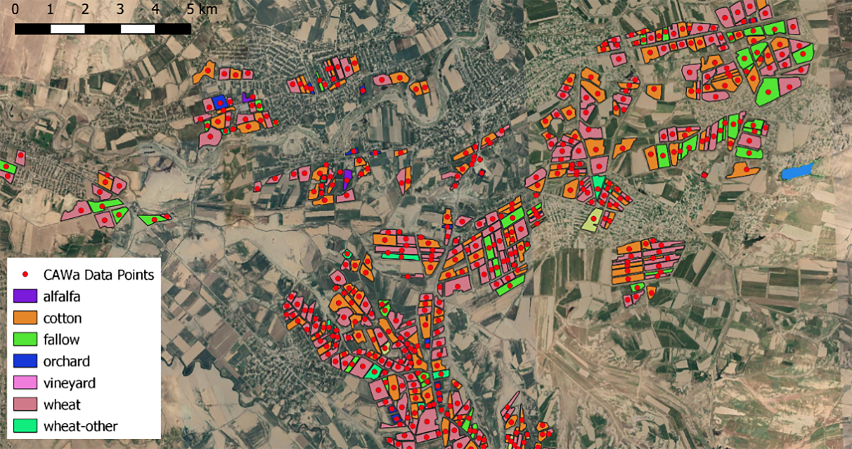
Figure 2.
Detail of the CAWa ground-truth reference data available for Kashkadarya. The map shows the polygons as provided by the CAWa dataset, as well as one point per polygon generated inside each shape.
Two supervised classifiers, the RF and the DTW were trained with monthly composites of Sentinel-1 and Sentinel-2 satellite images available from the period March to October 2018. Several rounds of training were performed using different numbers of randomly sampled training data points (5–10 points for DTW, 10–50 points for RF). We then applied the trained algorithms to classify all pixels of Kashkadarya region at a spatial resolution of 10 m, except for urban areas (based on the Copernicus Global Land Cover Layers
2.1.1Satellite data
Sentinel-2 L2A data and Sentinel-1 SAR GRD data were used in this study. Images acquired from March to October 2018 of each product were requested through GEE and selected bands were used as shown in Table 2.
Sentinel-1 SAR GRD was pre-processed using the angular-based radiometric slope correction for volume scattering from Vollrath et al., 2021 [5]. Indeed, Kashkardarya has a hilly landscape, and although crops cannot grow on very steep slopes, foreshortening and layover effects may still occur which can affect the interpretability of the data. Only the VV (Vertically transmit Vertically receive) polarization was used to reduce the number of input variables used. Although there seems to be an indication, at least in the case of winter wheat, that polarization and incidence angles have an influence in the retrieval of phenological stages [6], VV polarization has proven to be more determinant in general purpose cropland classification applications than VH polarization [7, 8], especially for distinguishing the vertical stem elongation phase of wheat [9], which is the dominant grain crop in the study area. Moreover, the combination of Sentinel-2 and Sentinel-1 acquisitions produces synergy in the sense that the Sentinel-2 time series data provides the most important variables for describing crop phenology, while Sentinel-1 can support the discrimination of cropland and crop types by providing a higher temporal density of observations in cloudy periods.
Sentinel-2 L2A data time series was pre-processed by performing cloud masking with s2cloudless probabilities [10] provided alongside the S2 L2A dataset on GEE. Only images with a cloudy pixel percentage inferior to 60% were requested, and a 40% cloud probability threshold on the s2cloudless dataset was applied for cloud masking. Moreover, the cloud shadow projection, calculated based on the mean solar azimuth angle and with a maximum search radius of 100 m, was used to identify cloud shadow pixels. Pixel values inferior to 0.15 NIR reflectance unit (band B8) and located inside the cloud shadow projection area were considered cloud shadow pixels, and therefore masked out. Finally, a morphological dilation of 100 m was applied to the resulting union between cloud mask and cloud shadow mask pixels to obtain the final cloud mask to apply to the original sentinel-2 image. As previously mentioned, there is a preference of over-masking rather than under-masking in the context of drylands to make sure any marginal cloud or haze pixels are removed. Besides, the relatively favourable observation conditions that the area exhibits, typically more than 40 cloud-free observation per year in agricultural regions, ensures that both quantity and quality of data are guaranteed. Bands B2, B3, B4, B8 (10 m) and B6, B11, B12 (20 m bands) were selected as input features. Normalized Difference Vegetation Index (NDVI) and the Enhanced Vegetation Index (EVI) were also generated as additional covariates and were used to model crop phenology.
2.2Temporal composites
Sentinel-1 and Sentinel-2 time series data are harmonized and reduced in size by implementing a temporal aggregation. Temporal aggregation requires a temporal interval parameter to be chosen, to generate (almost) cloud-free composites from all images within the chosen temporal interval. This results in a harmonized time series of equal-size temporal intervals if the same temporal interval is applied for the entire year. With knowledge of the crop calendar, different temporal intervals for aggregation can be chosen for different periods of the year, to get a denser profile around key crop growth stages between onset and senescence. We have tried both approaches:
1. Harmonized time series with 15-day composites, resulting in 16 composites for March-October 2018.
2. Harmonized time series with 30-day composites, and down to 10-day composites in the key growth stage periods as per national crop calendar information, namely from DOY 60 until DOY 150, and DOY 180 until DOY 270), also resulting in 16 composites for the period March October 2018. These figures are area-specific and are chosen to cover potential temporal shifts in the crop calendars across agro-ecological zones.
The geometric median was used to generate the temporal composites, as this preserves the spectral relationship between the composited bands, smoothens local spectral artefacts, and ensures consistency across scene boundaries.
As an alternative to temporal aggregation, data gaps could be filled spatially using a technique like the spectral angle mapper based spatio-temporal similarity (SAMSTS) developed by Yan and Roy in 2018 [11]. However, temporal aggregation was preferred to a gap-filling approach because data reduction was a desired outcome, considering the number of pheno-spectral input features used in this study. Based on the resulting temporal composites, the full extent of Kashkadarya region was deemed to have sufficient cloud-free observations in the span of a year, and therefore than no additional spatial-temporal gap filling was necessary.
2.3Harmonics fitting
After temporally aggregating data using a given temporal interval, data gaps and undesirable artefacts may remain in the data. While data gaps need to be filled, and artefacts need to be smoothened, the same method of time series harmonic fitting is suitable to address both issues. Also known as Fourier analysis, this method allows a complex curve to be expressed as the sum of a series of sine and cosine waves. Each wave is defined by a unique amplitude and a phase angle where the amplitude value is half the height of a wave, and the phase angle (or simply, phase) defines the offset between the origin and the peak of the wave over the range 0–2
Table 3
PA and UA for individual crop classes calculated using DTW (using 5 training samples per crop category) and RF ( 50 training samples per crop category) validated under Test A and Test B
| Test A | Test B | |||||||
|---|---|---|---|---|---|---|---|---|
| Class | PA-DTW | PA-RF | UA- DTW | UA-RF | PA-DTW | PA-RF | UA- DTW | UA-RF |
| Wheat | 83.50% | 83.00% | 99.00% | 99.10% | 90.00% | 90.00% | 84.40% | 87.10% |
| Cotton | 91.00% | 92.40% | 98.50% | 98.20% | 83.30% | 90.00% | 86.20% | 79.40% |
| Alfalfa | 53.30% | 70.00% | 50.00% | 31.30% | 53.30% | 70.00% | 80.00% | 72.40% |
| Orchard | 27.30% | 51.50% | 20.90% | 31.50% | 26.70% | 50.00% | 61.50% | 65.20% |
| Vineyard | 73.30% | 80.00% | 33.30% | 39.30% | 73.30% | 80.00% | 61.10% | 66.70% |
| Wheat-other | 93.30% | 96.70% | 34.60% | 31.90% | 93.30% | 96.70% | 87.50% | 85.30% |
| Non-crop | 78.70% | 59.60% | 22.70% | 27.20% | 86.70% | 56.70% | 54.20% | 73.90% |
2.4Pheno-spectral feature extraction – crop reference signature
The fitted time series generated provide us with phenology of all land surfaces in the Kashkadarya region at a pixel level. To better characterize the phenology of the different surfaces, namely those of crop, phenological stages can be extracted from the time series [14]. The main advantage of extracting phenological stages is to be able to visually, as well as well as algorithmically, separate crops with distinct crop calendars. Moreover, considering the representativeness of the phenological stages extracted, the spectral values of Sentinel-1 VV channel, Sentinel-2 bands and vegetation indices corresponding to the DOY at which the phenological stages were extracted to provide additional meaningful input features to discriminate between crop types, also referred to as pheno-spectral features. The use of phenological stages alone may be subject to the inter-annual and inter-regional variation of crop calendar, but including the dynamic spectral properties of pheno-spectral features offers a more reliable identification of different crop types. The phenological stages extracted, as well as their corresponding pheno-spectral features, are summarized in Table 2. One can appreciate the resulting data reduction of using extracted phenological stages and pheno-spectral features, as opposed to raw time series (Table 3), while ensuring optimal discrimination of the targeted crop types. Considering the operational nature of the conceived system, data size and processing time are of concerns, and any data reduction that does not significantly affect the quality of the produced output is considered. The results of the extraction of the pheno-spectral signature were used to build a library of crop reference signatures.
2.5Classification algorithms
Two supervised classification algorithms were used for the generation of the crop maps: i) time-constrained Dynamic Time Warping (DTW) and ii) Random Forest (RF) supervised classification. The algorithms underwent through several rounds of training using different numbers of randomly sampled training samples (5–10 points for DTW, 10–50 points for RF). The trained algorithms were in turn used to classify all pixels of Kashkadarya region at a spatial resolution of 10 m, except for urban areas (based on the Copernicus Global Land Cover Layers), or pixels above a certain elevation (2500 m above sea level) or with steep slopes (
2.6Time-constrained dynamic time warping
We used a DTW algorithm to simulate condition of scarce availability of in-situ data. The DTW algorithm classifies every pixel in the study area by comparing the spectral signature of that pixel to that of the reference crops contained in the crop library. The DTW measures the similarity between two temporal data sequences by identifying their optimal alignment and by producing a dissimilarity index (Fig. 3). Computing the alignment between two sequences is done recursively using the DTW matrix. The algorithm picks the smallest DTW dissimilarity value between the query pattern and the available reference patterns and attributes the corresponding reference crop label to the pixel.
Figure 3.
Computing the alignment between two sequences at hypothetical test areas (TA) TA1 andTA2. The vertical and horizontal values of the DTW matrix represent the date of an image. The alignment between two sequences is computed only for the yellow cells of the matrix, reducing the number of computations necessary (a maximum time delay, w, of 45 days is used in this example). After computing the matrix from upper left to lower right, the last element of the matrix, m[S,T], is returned, as a measure of DTW dissimilarity between the two compared sequences. Image credits: Csillik et al. [16].
![Computing the alignment between two sequences at hypothetical test areas (TA) TA1 andTA2. The vertical and horizontal values of the DTW matrix represent the date of an image. The alignment between two sequences is computed only for the yellow cells of the matrix, reducing the number of computations necessary (a maximum time delay, w, of 45 days is used in this example). After computing the matrix from upper left to lower right, the last element of the matrix, m[S,T], is returned, as a measure of DTW dissimilarity between the two compared sequences. Image credits: Csillik et al. [16].](https://content.iospress.com:443/media/sji/2022/38-3/sji-38-3-sji220054/sji-38-sji220054-g003.jpg)
DTW classification has the main advantage that only a small number of training samples are required to build the crop reference library. According to Belgiu and Csillik [15, 16] as little as 3 samples per crop type. This is a big advantage for regional and national crop type mapping, especially in countries which lack in-situ data of adequate quality. A few clean reference samples that represent the characteristic temporal pattern of the crop type are sufficient for the DTW to function. Conversely, the positional accuracy and correctness of the crop label of the training data is of paramount importance for DTW, as the algorithm is very sensitive to errors in the training data.
A time-flexible method for comparing two temporal patterns by considering their temporal distortions in their alignment, the DTW has proven to achieve better results than the Euclidean distance measure for NDVI time series clustering [17]. This flexibility is desirable for crop mapping, to deal with the intra-class phenological discrepancies caused by different agricultural practices, environmental conditions, or by different weather conditions. This is beneficial also for comparisons among samples which are more geographically distant than the pixel to be classified, as they may exhibit temporal shifts in growing patterns, while still belonging to the same crop type class for computing DTW. It is apply time constraints considering the specific seasonality of different crops. For example, comparing an element of a sequence with all other elements of another sequence leads to erroneous results when aligning a winter crop with a summer crop. Applying time constraints on time warping increases the speed of processing, while providing meaningful results. A so-called time constrained DTW implementation was therefore used in our study. The elements of two time series will be compared only if the date difference is smaller or equal to
2.7Random forest
Random forest is an ensemble learning method for classification that operates by constructing a multitude of decision trees based on available training data as shown in Fig. 4 [17].
Figure 4.
Workflow of the random forest classification.
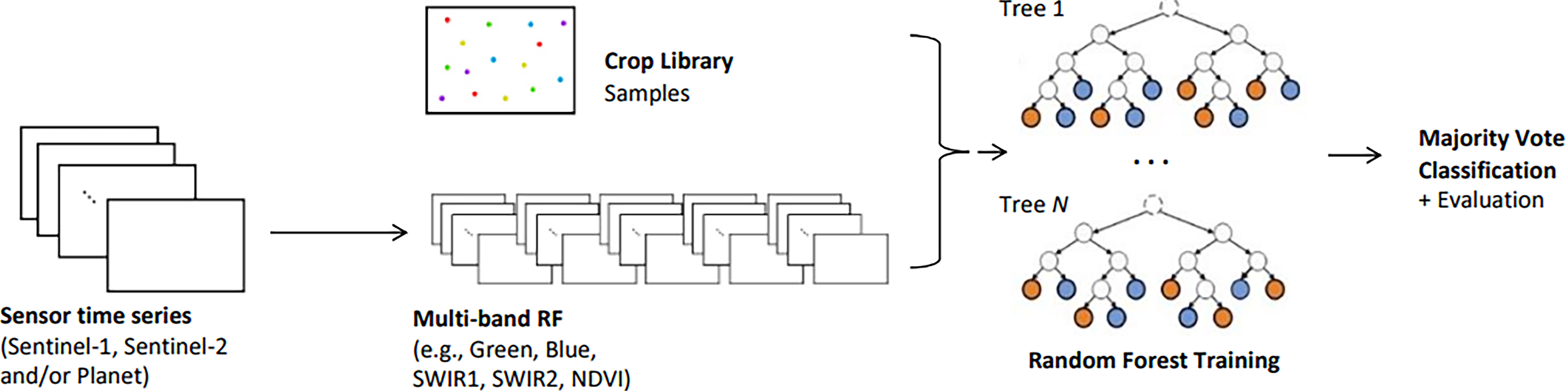
In a multi-band RF, the number of variables available for tree construction is
2.8Accuracy test
In order to compare the performance of the two classifies in producing accurate crop type maps, we have initially trained the DTW using 5 and 10 training and produced the respective crop maps. Then we have trained the RF using 5, 10, 20, 30, 40 and 50 training samples and produced the respective crop maps. In line with recommendations from Foody [23] and Congalton [24, 25], we evaluated the accuracy of the DTF and the RF through the establishment of confusion matrixes using two different settings: i) we used all of the validation data (Test A), and ii) we used only 30 validation samples (Test B). The Overall accuracy (OA), the Producer Accuracy (PA), the User Accuracy (UA), were computed for each map produced by the DTW and the RF under both Test 1 and Test 2.
The PA is the map accuracy from the point of view of the map maker (the producer). It measures how often are the ground-truth features correctly shown on the classified map, or the probability that a certain land cover of an area on the ground is classified as such. The PA is the complement of the Omission Error, PA
The UA is the probability that a value predicted in the map to be really belonging to that class. The User’s Accuracy is the complement of the Commission Error, UA
The OA is the probability that an individual will be correctly classified by a test; that is, the sum of the true positives plus true negatives divided by the total number of individuals tested.
The OA’s obtained from the validation of the maps produced by the DTW and RF classifiers were finally analyzed in function of the number of training samples used, for both Test A and Test B.
Table 4
Classified areas per crop category in km
| Area [km | Area [% of total crop area] | Area [km | Area [% of total crop area] | Difference (RF – DTW) | ||
| Crop class | DTW | DTW | RF | RF | [km | [%] |
| Wheat | 1446.7 | 33.41% | 1480.1 | 26.64% | 33.4 | 2.31% |
| Cotton | 1421.1 | 32.82% | 1626.2 | 29.27% | 205.1 | 14.43% |
| Alfalfa | 221.2 | 5.11% | 867.8 | 15.62% | 646.5 | 292.27% |
| Orchard | 606.2 | 14.00% | 883 | 15.89% | 276.8 | 45.66% |
| Vineyard | 461.5 | 10.66% | 502.4 | 9.04% | 40.9 | 8.86% |
| Wheat-other | 173.9 | 4.02% | 197.1 | 3.55% | 23.2 | 13.34% |
| Total Crops | 4330.6 | 25.49% | 5556.5 | 32.70% | 1226 | 22.06% |
| No-crop | 12659.7 | 74.51% | 11433.8 | 67.30% | 1226 | |
| Total area | 16990.3 | 100% | 16990.3 | 100% | ||
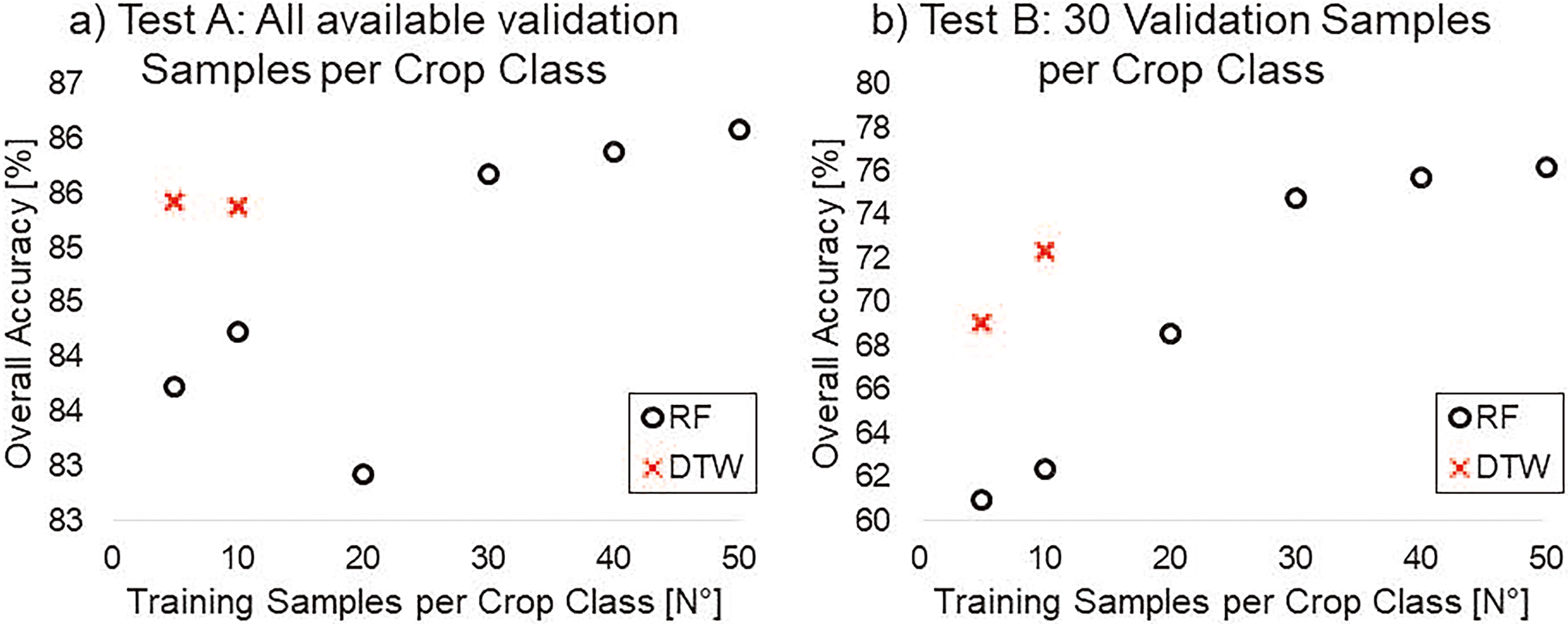
Figure 5.
Overall accuracy of the DTW and RF classifiers as a function of the number of training samples used. In a) all validation data points were used to assess the OA. In b) only 30 validation data points were used to assess the OA. In both a) and b) the DTW scores significantly higher OA than to RF, when 5 to 20 samples are used for training. Only when 30 or more training samples are used, the RF scores higher OA compared to DTW.
3.Main results
The maps obtained from the different runs of the DTW and the RF, trained with increasing number of training points (from 5 to 50), were tested for OA using all the validation samples (Test A), and using a random subset of only 30 validation samples (Test B), ti simulate lack of validation data (Fig. 5).
Under Test A, when 5 and 10 samples were used for training, DTW scored an OA of 85.43% and 85.38 respectively, while RF scored a lower OA of 83.73% and 84.23%. When using 20, 30, 40, and 50 training data samples the RF scored an OA of 82.93%, 85.68%, 85.88%, and 86.08% respectively. Under Test B, when 5 and 10 samples were used for training, DTW scored an OA of 69.05% and 72.38% respectively, while RF scored a lower OA of 60.95% and 62.38%. When using 30, 40, and 50 training data samples the RF scored an OA of 68.57%, 74.76%, 75.71% and 76.19 respectively. The highest OA was scored by the DTW when 5 training samples were used, and by the RF when 50 training samples were used under Test 1 and under Test 2. Overall, when trained with a very low number of training samples (from 5 to 10), the DTW scores higher OA than the RF (
The crop classes’ specific PA and UA for the best runs of the DTW (5 training samples) and the RF (50 training samples), are compared under Test 1 and Test 2, as shown in Table 3.
Under Test A, both DTW and RF, score the highest UA for wheat (99% and 99.1%) and for cotton (98.5% and 98.2%). The values are very similar for both algorithms, which is indicative that they produce an extremely low rate of commission errors (false positives) for the two dominant crop classes in the Kashkadarya region. The PA for these two classes is also quite high for both the DTW and the RF (wheat 83.5% and 83%; cotton 91% and 92.4%) indicating a low rate of omission errors.
The UA scores for the minor crop classes are overall low for both the algorithms which is not surprising as these crop classes are rare to find DTW performs better for alfa-alfa (50% UA vs 31.30% UA) and for wheat-other (34.6% UA vs 31.9% UA) while RF performs better for orchard (31.5% UA vs 20.9% UA) and vineyard (39.3% vs 33.3% UA). No-crop class scored a UA of 22.7% for DTW and 27.2% for RF, which denotes an underestimation of this class by both classifiers. The PA for the minor classes is overall higher for RF. Only in the case of the non-crop the PA for DTW is higher (78.7% vs 59.6%).
Under Test B, the UA for the dominant crops (wheat and cotton) is significantly lower for both the DTW and the RF compared to Test A. Wheat scores a higher UA for RF (87.1%) compared to DTW (84.4%) and cotton scores a higher UA for DTW (83.2%) than the RF (79.4%). Minor crops’ UA is significantly higher in Test B for both DTW and RF than in Test A. PA for alfa-alfa and wheat-other is higher for DTW (80% and 87.5%) than for RF (85.3% and 77.4%). UA for orchard and vineyard is higher for RF (65.2 and 66.7%) than for DTW (61.5% and 61.1%) The UA for non-crop is significantly higher in RF (73.9%) than the DTW (54.2%).
The non-crop class is the largest land use category and the capacity of the RF and the DTW models to accurately predict this class has a direct impact on the estimation of the total crop area (Table 4). According to the DTW 74.51% of the total classified area is non-crop, whereas according to the RF only 67.3%.
According to DTW, 25.49% of the total classified areas are used for crop cultivation and 32.7% according to RF. With the RF, we obtain a total crop area that is 22.06% larger than the area calculated with the DTW. The major contribution to such difference stems from the difference in alfalfa acreages, which are almost three times larger based on the RF classifier (Table 4). Alfalfa represents only 0.6% of the reference data polygons, but 15.6% of the classified crop areas with RF (DTW: 5.1%). It is likely that both classifiers thus overestimate the total alfalfa acreages.
4.Conclusions
This assessment has demonstrated that the crop classification obtained using the DTW on 5 training samples outperforms conventional RF classification only when using a number of training samples five times higher. However, even in these conditions, the RF yields land cover estimates of the ‘no-crop’ category with a higher user accuracy that the DTW, while the DTW performs better 556 bis in terms of producer accuracy (Table 3 Test B). The “no crop” category is underrepresented in the ground-truth dataset used for validation, but is generally the most important category for estimating the total crop acreages, because it is the most abundant land cover type in Kashkadarya region. RF estimated a non-crop area of 11433.8 km
We conclude from these results that the DTW lead to more accurate and more robust results than RF in those contexts where limited in-situ data are available (5 to 20 trining samples). The main condition for obtaining good results with supervised classifier is the quality of the training data, specifically the attribute accuracy and the location accuracy. In the case of the DTW the quality assurance and quality control of the training samples assumes an even higher role due to the fact that only few points are used. Even in a published crop type dataset, such as the one used for this assessment, we found several misclassifications that could be explained with timing of the field campaign (June 2018), which was likely too early in the year for accurate sampling of late crops, or with incorrect delineations of the field boundaries. While the full ground-truth dataset consists of 2,172 samples, we only needed 40–80 samples to train the DTW algorithm. It is understood that the quality assurance and control of such small samples sizes requires less time and can therefore be carried out more thoroughly. On the other hand, the RF classifier is less sensitive to noise in the training data, and when a large training data set is used, it can compensate for possible mistakes in the labeling of the ground-truth data. However, as discussed initially, a large number of training samples are difficult to obtain, especially in poor countries. In conclusion, we argue therefore that the DTW, as implemented in the EOSTAT CropMapper, is a valuable alternative to the RF classification in the context of in-situ data scarcity.
References
[1] | Kam H. Random decision forests. Proceedings of 3rd International Conference on Document Analysis and Recognition. (1995) . |
[2] | Petitjean F, Ketterlin A, Gancarski P. A global averaging method for dynamic time warping, with applications to clustering. Pattern Recognition. (2011) . |
[3] | Remelgado R, Zaitov S, Kenjabaev S et al. A crop type dataset for consistent land cover classification in Central Asia. Sci Data. (2020) ; 250: : 7. |
[4] | FAOSTAT Crop Mapper application. https://ocsgeospatial.users.earthengine.app/view/eostat-afghanistan. |
[5] | Vollrath A, Adugna M, Johannes R. Angular-based radiometric slope correction for Sentinel-1 on google earth engine. Remote Sensing. (2020) . |
[6] | Nasrallah A, Baghdadi N, El Hajj T, Darwish T, Belhouchette H, Faour G, Darwich S, Mhawej M. Sentinel-1 Data for Winter Wheat Phenology Monitoring and Mapping. Remote Sens. (2019) ; 11: : 2228. |
[7] | Erkki T, Antropov O, Praks J. Cropland classification using Sentinel-1 time series: Methodological performance and prediction uncertainty assessment. Remote Sensing. (2019) ; 248: . |
[8] | Inglada J, Vincent A, Arias M, Sicre C. Improved Early Crop Type Identification By Joint Use of High Temporal Resolution SAR And Optical Image Time Series. Remote Sensing. (2016) ; 362: : (8). doi: 10.3390/rs8050362. |
[9] | Roberts DR, Ciuti S, Boyce MS, Elith J, Guillera-Arroita G, Hauenstein S, Lahoz-Monfort JJ, Schröder B, Thuiller W, Warton DI, Wintle BA, Hartig F, Dormann CF. Cross-validation strategies for data with temporal, spatial, hierarchical, or phylogenetic structure. Ecography. (2017) ; 40: : 913-929. |
[10] | Zupanc A. Improving Cloud Detection with Machine Learning. Sentinel Hub Blog. (2017) . https://medium.com/sentinel-hub/improving-cloud-detection-with-machine-learning-c09dc5d7cf13. |
[11] | Yan L, Roy DP. Robust large-area gap filling of Landsat reflectance time series by spectral-angle-mapper based spatio-temporal similarity (SAMSTS). Remote Sensing. (2018) ; 10(4): : 609. |
[12] | Trong HN, Nguyen TD, Kappas M. Land Cover and Forest Type Classification by Values of Vegetation Indices and Forest Structure of Tropical Lowland Forests in Central Vietnam. International Journal of Forestry Research,(2020) . |
[13] | Qiu Y, Zhou J, Chen J, Chen X. Spatiotemporal fusion method to simultaneously generate full-length normalized difference vegetation index time series (SSFIT). International Journal of Applied Earth Observation and Geoinformation. (2021) ; 100: . |
[14] | Zhong L, Hu L, Yu L, Gong P, Biging G. Automated mapping of soybean and corn using phenology. ISPRS Journal of Photogrammetry and Remote Sensing. (2016) . |
[15] | Belgiu M, Csillik O. Sentinel-2 cropland mapping using pixel-based and object-based time-weighted dynamic time warping analysis. Remote sensing of environment. (2018) ; 204: : 509-523. |
[16] | Csillik O, Belgiu M, Asner GP, Kelly M. Object-based time-constrained dynamic time warping classification of crops using Sentinel-2. Remote Sens. (2019) ; 11: . |
[17] | Zhang Z, Tanb P, Huo L-Z, Zhou Z-G. MODIS NDVI time series clustering under dynamic time warping. International Journal of Wavelets, Multiresolution and Information Processin. (2014) ; 12: . |
[18] | Tatsumi K, Yamashiki Y, Canales Torres M, Ramos C. Crop classification of upland fields using Random forest of time-series Landsat 7 ETM+ data. Computers and Electronics in Agriculture. (2015) ; 15: . |
[19] | Defourny P, Bontemps S, Bellemans C, Dedieu G, Guzzonato E et al. Near real-time agriculture monitoring at national scale at parcel resolution: Performance assessment of the Sen2-Agri automated system in various cropping systems around the world. Remote Sensing of Environment. (2019) ; 221: : 551-568. |
[20] | Orynbaikyzy A, Gessner U, Mack B, Conrad C. Crop Type Classification Using Fusion ofSentinel-1 and Sentinel-2 Data: Assessing the Impact of Feature Selection, Optical Data Availability, and Parcel Sizes on the Accuracies. Remote Sensing. (2002) ; 12: . |
[21] | Fan J., Defourny P, Zhang X, Dong Q, Wang L, Qin Z, DeVroey M, Zhao C. Crop Mapping with Combined Use of European and Chinese Satellite Data. Remote Sens. (2021) ; 13: : 4641. |
[22] | Sherrie W, George A, David B, Dong Q, Wang L, Qin Z, DeVroey M, Zhao C. Lobell, Crop type mapping without field-level labels: Random forest transfer and unsupervised clustering techniques. Remote Sensing of Environment. (2019) . |
[23] | Foody GM. Explaining the unsuitability of the kappa coefficient in the assessment and comparison of the accuracy of thematic maps obtained by image classification. Remote Sens. Environ. (2020) ; 239: : 111630. |
[24] | Congalton RG. A review of assessing the accuracy of classifications of remotely sensed data. Int. J. Remote Sens. (1991) ; 37: : 35-46. |
[25] | Congalton RG, Green K. Assessing the Accuracy of Remotely Sensed Data: Principles and Practices, 2nd ed. CRC Press/Taylor & Francis: BocaRaton, FL, USA. (2009) . |


