
Alternative methods for disaggregating Sustainable Development Goal indicators using survey data
Abstract
Samples used in most surveys are either not large enough to guarantee reliable direct estimates for all relevant sub-populations, or do not cover all possible disaggregation domains. After having described a holistic strategy for producing disaggregated estimates of Sustainable Development Goal (SDG) indicators, this paper discusses alternative sampling and estimation methods that can be applied when sample surveys are the primary data source.
In particular, the paper focuses on strategies that can be implemented at different stages of the statistical production process. At the design stage, the paper describes a series of sampling approaches that ensure a “sufficient” sampling size for each disaggregation domain. In this context, the article highlights the main limitations of traditional sampling approaches and shows how ad-hoc techniques could overcome some of their key constraints. At the analysis stage, it discusses an indirect model-assisted estimation approach to integrate data from independent surveys and censuses, eliminating costs deriving from redesigning data collection instruments, and ensuring a greater accuracy of the final disaggregated estimates. A case study applying the abovementioned method on the production of disaggregated estimates of SDG Indicator 2.1.2 (Prevalence of Moderate and Severe Food Insecurity) is then presented along with its main results.
1.Introduction
With the adoption of the Leave No-one Behind principle as central pledge of the 2030 Agenda for Sustainable Development, the United Nations Member States have committed to reduce inequalities and vulnerabilities within their country for all Sustainable Development Goal (SDG) targets. The SDG indicators, consequently, need to be disaggregated by multiple dimensions in order to monitor all relevant population groups and geographical areas. In order to operationalize the overarching requirement of data disaggregation in the development of the Global Indicator Framework, the United Nations Statistical Commission (UNSC) specified that: “SDG Indicators should be disaggregated, where relevant, by income, sex, age, race, ethnicity, migratory status, disability and geographic location, or other characteristics, in accordance with the Fundamental Principles of Official Statistics”.
Producing high quality disaggregated estimates of SDG indicators imposes significant challenges to National Statistical Systems (NSSs), both in terms of data requirements and operational complexity. With this in mind, at its Forty-Seventh Session, the UNSC requested the Inter-Agency and Expert Group on SDG Indicators to form a working group (WG) on data disaggregation aimed at developing the necessary statistical standards and tools to produce disaggregated data and at strengthening national capacities to implement them. Among the key outputs developed so far, the WG has identified for each target the policy priorities targeting the most vulnerable population groups and the related main disaggregation categories and dimensions for the official SDG indicators monitoring that target.
Within this context, the Food and Agriculture Organization of the United Nations (FAO), an active member of the WG, has recently published the Guidelines on data disaggregation for SDG indicators using survey data [1], which provide comprehensive methodological and practical guidance on producing disaggregated estimates for the SDG indicators having surveys as their primary data source.
The FAO Guidelines [1] promote a holistic approach to data disaggregation, which involves the formulation of a strategic plan for the integrated use of alternative approaches, statistical methods and tools at different stages of the statistical production chain. The strategic plan foresees a set of actions that can be grouped under four main pillars: (1) Actions at the strategic level that establish the strategic choices for data disaggregation, which in turn determine the activities conducted at the technical level. (2) Actions at the sampling design level aimed at defining sample designs that can guarantee the production of disaggregated data with controlled quality for relevant domains. (3) Actions at the direct estimation level to (i) measure sampling accuracy and (ii) improve the quality of direct estimates, including by defining auxiliary variables that can be used both for benchmarking sampling estimates and correcting sampling non-response. (4) Actions at the indirect estimation level that can be implemented when direct estimates perform poorly. The ultimate objective of all actions is to enable NSSs to regularly produce and disseminate SDG data at a more detailed level and, eventually, improve governments’ decision-making processes.
This paper, within the framework described in [1], presents the main results and findings of FAO’s research activities on data disaggregation covering actions (2) and (4) outlined above. Section 2 describes a series of traditional and more sophisticated sampling strategies that ensure a “sufficient” number of sampling units for each disaggregation domain. Section 3 addresses data disaggregation at the analysis stage, discussing a model-assisted indirect estimation method based on the application of the so-called projection estimator [2]. This method allows integrating a small survey, measuring a target variable with a small measurement error, and a more extensive survey, collecting variables of general use (e.g. socio-demographic and economic auxiliary variables). Section 3 also presents the results of a case study relying on the use of the projection estimator to produce model-assisted disaggregated estimates of SDG indicators 2.1.2 on the Prevalence of Moderate and Severe Food Insecurity based on the Food Insecurity Experience Scale (FIES). Finally, some concluding remarks and recommendations for future work are illustrated in Section 4.
2.Planning for data disaggregation at the survey design phase
In order to produce direct disaggregated estimates, the selected sampling design should foresee a planned sample size in each disaggregation domain. The presence of sampling units in all disaggregation domains can also enhance the production of indirect estimates through a substantial reduction of the model bias. When members of a rare sub-population (or domain) can be identified from the sampling frame, selecting the required sample size for the relevant domain is relatively straightforward. In such cases, the main issue is the extent of oversampling to employ for achieving the targeted level of accuracy in each disaggregation domain [3].
Sampling and oversampling rare domains whose members cannot be identified in advance, instead, present major challenges. A variety of methods have been used in these situations. In addition to large-scale screening, these approaches include disproportionate stratified sampling, two-phase sampling, the use of multiple frames, multiplicity sampling, and location sampling. Traditional sampling techniques address data disaggregation by oversampling or introducing deeper stratification. More sophisticated techniques allow for improving sampling designs by geographically spreading the sample units [4] and reducing the level of clustering. These approaches help reaching isolated or rare subpopulations. In general, traditional sampling techniques present a number of issues when dealing with rare subpopulations [3]. The classification of disaggregation domains could be based on their relative size with respect to the total population [5]. The author identifies as “major domains” those comprising at least 10 per cent of the total population. For major domains, a traditional sampling design should normally produce reliable estimates. “Minor domains” are those containing from 1 to 10 per cent of the total population. In these cases, special sampling approaches are needed to ensure a sufficient sampling size. “Mini-domains” include from 0.1 to 1 per cent of the total population, and require the use of statistical models in order to get reliable estimates. Finally, “rare domains”, comprising less than 0.1 per cent of the total population, cannot be handled with survey sampling methods.
Issues also arise with populations that are hard to reach or elusive (such as the irregular workers, the homeless, the migrants, or nomadic populations) [6]. For example, in designing a survey for pastoral activities in developing countries we would need to collect data on nomadic populations, which can be very hard to locate [7]. New approaches recently developed in the sampling literature allow some of the abovementioned problems to be overcome. These methods are, for instance, indirect or multisource sampling [8, 9, 10, 11] or marginal stratification sampling [12, 13]. These approaches are extensively discussed in the FAO Guidelines [1] and summarized in Sections 3.1 and 3.2 of this paper.
Table 1
Effect on domain sample size nd due to an increase Δ of the initial sample size n (10000 households) by domain relative size Pd
| Pd % | ||||
|---|---|---|---|---|
| Δ | 0.05% | 1% | 5% | 10% |
| 10% | 5 | 10 | 50 | 100 |
| 50% | 25 | 50 | 250 | 500 |
| 100% | 50 | 100 | 500 | 1.000 |
Source: [1].
2.1Traditional sampling techniques to address data disaggregation
2.1.1Oversampling
With oversampling, a larger size of the overall original sample is defined. This, in turns, results in a larger sample size at the domain level. If the initial sample size n is augmented by a proportion Δ, this is expected to have an impact on the increase of the domain sample size equal to nΔPd, where Pd=Nd/N is the relative size of the domain d. Table 1 represents the expected increase in the domain sample size nd due to a percentage increase Δ in the overall sample size of 10.000 households by different subpopulation proportions. Table 1 shows that oversampling may be useful when dealing with major domains [5]. On the other hand, this approach is not ideal, and potentially unsustainable, when dealing with minor, mini and rare domains. In addition, when the disaggregation domain is not planned at the sampling design stage, the result of oversampling is uncertain, as the domain sample size achieved may be different from the expected one. Table 2 illustrates the overall sample size n needed to guarantee the minimum acceptable size n∗d, for different values of n∗d and the subpopulation proportion Pd. It can be seen that, in order to achieve the required n∗d for rare subpopulations (Pd⩽ 1%), the overall sample size would need to be way too large and substantially unfeasible for most surveys conducted at national level.
Table 2
Sample size
| % | ||||
|---|---|---|---|---|
|
| 0.05% | 1% | 5% | 10% |
| 30 | 62.000 | 31.000 | 6.200 | 3.100 |
| 50 | 102.000 | 51.000 | 10.200 | 5.100 |
| 100 | 202.000 | 101.000 | 20.200 | 10.100 |
Source: [1].
2.1.2Deeper stratification
Stratifying by disaggregation domain is the traditional strategy adopted to control the sample size
2.1.3Multiphase sampling with a screening of respondents
The strategy based on a deeper stratification requires the availability of the domain variables
A traditional sampling strategy to overcome this problem is to select a first-phase sample
2.2Alternative sampling techniques to address data disaggregation
2.2.1Marginal stratification designs
The literature on sampling designs provides various methods to keep under control the sample size in all categories of the stratifying variables without using a cross-classification design. These methods are generally referred to as multi-way stratification techniques and have been developed under two main approaches: (i) the Latin Squares or Latin Lattices schemes [15]; and (ii) controlled rounding problems via linear programming [16]. Both approaches present drawbacks that have limited the use of multi-way stratification techniques as a standard solution when planning survey sampling designs in real survey contexts. The main weakness of the linear programming approach is its computational complexity. The sampling strategy proposed below, based on balanced sampling, does not suffer from the disadvantages of the abovementioned methods and grants control over the sample size of various disaggregation domains of interest, defined by different partitions of the reference population. Furthermore, it guarantees that the sampling errors of domain estimates are lower than a predefined threshold. To define the balanced sampling in the design or model-assisted approach, let us introduce the general definition of sampling design as a probability distribution
(1)
such that
(2)
where
(3)
where
When defining the vector
The left-hand side of the balancing Eq. (1) is
where
The right-hand side of the balancing equation is
Tillé [17] proposes the cube method that allows for the selection of balanced (or approximately balanced) samples for a large set of auxiliary variables and with respect to different vectors of inclusion probabilities. In particular, Deville and Tillé [18] show that with
It is important to notice that balanced sampling provides the basis to define broad classes of sampling designs. For example, stratified sampling designs require that:
and each
Table 3
Example of marginal stratification design: Selected municipalities and sample of individuals in each cross-classification cell
| Place of residence by degree of urbanization | ||||
|---|---|---|---|---|
| Region | Rural | Urban, non- metropolitan | Metropolitan | Total sample |
| Region 1 | 1 (305) | 0 | 1 (150) | 2 (500) |
| Region 2 | 1 (75) | 1 (175) | 0 | 2 (250) |
| Region 3 | 0 | 1 (20) | 1 (80) | 2 (100) |
| Region 4 | 1 (80) | 0 | 1 (70) | 2 (150) |
| Total sample | 3 (505) | 2 (195) | 3 (300) | 8 (1.000) |
Source: [1].
2.2.2Indirect sampling
In any conventional survey, random selection of the sample requires an updated list that records all individuals eligible for the survey (and only them), each identified by a label. This perfect list, i.e. the sampling frame, is used to identify the elements of the target population. When the sampling frame is available, a crucial statistical issue is the assessment of the coverage actually provided by this list of the target population. A sampling frame is perfect when there is a one-to-one mapping of frame elements to target population elements. However, in the statistical practice, perfect frames seldom exist, and problems always arise disrupting the ideal one-to-one correspondence. For example, the sampling frame might suffer from either under-coverage or over-coverage. There is under-coverage when the available frame is incomplete, because it includes only part of the target population, and the missing elements cannot appear in any sample drawn for the survey. On the other hand, there is over-coverage when the sampling frame contains duplications of the same units or units that are not included in the target population. However, there may also be frame imperfections of other kinds: for example, in certain circumstances, a frame of the desired collection units may not be available, but rather another frame of units linked to the list of units of interest. Also, although a frame may be available, in a dynamic environment it quickly becomes outdated, thus representing a situation that might be rather different from reality. In order to address this problem, the following strategy may be adopted: selecting the units from the population with the available frame, the units of the other populations are indirectly surveyed exploiting their links with the units of the first population. Thus, as it would occur with an indirect sampling approach, the other populations can be considered sampled from an imperfect frame, i.e. the frame referring to the first population. Frame imperfections will also be considered in the observation of the first population. Figure 1, taken from the FAO Guidelines on the Integrated Survey Framework [9], illustrates the links in the case of a farm survey when only a list of households, derived from the last census, is available. In practice, the links do not have to be known in advance as the enumerator obtains this information during the data collection phase. For instance, consider that in Fig. 1, the enumerator who interviews individuals A and B of Household H1 identifies two links between Household H1 and Farm F1. In addition, links with Farm F1 can also be identified by the enumerator interviewing individual E in Household H2. Hence, Farm F1 may be identified by a total of three links, each of which can be detected during the data collection. This is an example of the concept of multiplicity discussed below. To identify these links, survey questionnaires must be appropriately structured. The FAO Guidelines on the Integrated Survey Framework [9] illustrate the modules and operational rules for applying indirect sampling in agricultural surveys.
Figure 1.
Example of links between a frame of households and the target population of agricultural holdings in the household sector (Source: [9]).
![Example of links between a frame of households and the target population of agricultural holdings in the household sector (Source: [9]).](https://content.iospress.com:443/media/sji/2022/38-2/sji-38-2-sji210901/sji-38-sji210901-g001.jpg)
It should be noted that, in its simplest formulation, indirect sampling may fail the goal of ensuring that a sufficient sample size is attained. The problem comes from the nature of indirect selection itself: the final sample size on the target population based on a sample selected from a sampling frame referred to another population is difficult to predict. [13] proposes a solution to this problem that minimizes the sampling cost, ensuring a predefined estimation precision for the variables of interest. The method is specified for different contexts characterizing the information on the links available at the sampling design stage, ranging from situations where the relations among units are known at the design phase to conditions where there is limited information on the links. Moreover, adaptive cluster-sampling, a particular variant of indirect sampling [10], is a powerful tool to reduce the cost of screening for rare subpopulations when information on households’ neighborhoods is available. The efficiency gains of adaptive cluster sampling result from screening fewer households for the same number of homes as would be identified had adaptive cluster sampling not been used. A version of the methodology has been used in several European countries as part of the Second European Union Minorities and Discrimination Survey [20].
2.2.3Multisource sampling
Multisource sampling is another useful approach when dealing with imperfect frames, in particular, when the target population is defined by the combination of two or more frames. A relevant example here is that of agricultural surveys covering holdings in the household and non-household sector. In some circumstances, some of the holdings may fall under two different frames, that of the household sector and that of businesses that are legal entities.
Considering two partially overlapping frames A and B, if a sample
![Implementation of the projection estimator (Source: [1]).](https://content.iospress.com:443/media/sji/2022/38-2/sji-38-2-sji210901/sji-38-sji210901-g002.jpg)
3.Addressing data disaggregation at the analysis stage
3.1The projection estimator
At the analysis stage, data disaggregation can be addressed by adopting indirect estimation approaches11 coping with the little information available for so-called small domains and borrowing strength from additional domains. The indirect estimators allow producing estimates of a parameter of interest for a given estimation domain, by integrating sample data pertaining to that domain with additional information coming either from different domains or alternative data sources. In particular, the integrated use of different data sources offers a powerful approach for achieving the desired level of disaggregation while preserving estimates accuracy. Typical data sources that could be integrated with data from a particular household and/or agriculture survey are other surveys, censuses, administrative registers, geospatial information and big data.
Indirect estimation approaches range from model-based to model-assisted approaches. Among the various methods available to produce indirect estimates, this paper uses a model-assisted approach based on the so-called “Projection estimator” [2]. The method (Fig. 2) allows integrating data from two independent sample surveys – or a sample survey and a census – where the first survey is characterized by a large sample
(4)
where
This method can be adopted in a great deal of possible empirical situations relevant to data disaggregation. As a matter of fact, most countries have at least one large-scale survey collecting general-use variables, such as censuses, household surveys, but also administrative registers. On the other hand, some of the target variables to be disaggregated in the context of the SDGs are too costly to be measured with a large-scale survey. In these circumstances, a possible solution could be to measure the phenomenon of interest using a small-scale survey and then improve estimates accuracy by means of a working model relying on auxiliary information collected through a larger-scale survey. The only two requirements to be satisfied for the implementation of this approach are that the two surveys must share the same set of auxiliary variables used to fit the regression model, and that these are good predictors of the variable of interest. This approach allows disaggregating the indicator of interest by dimensions not included in the small survey (e.g. indigenous status, even if only collected on the large sample). Furthermore, integrating a small sample from a non-official source with a larger one from an official national survey, strongly increases the consistency of the disaggregated SDG indicators with the official disseminated statistics. For instance, this allows obtaining identical population totals for sex and age or regions.
In many cases, SDG indicators based on survey data present the following functional form:
where
(5)
where
is the direct estimate of the total
(6)
where
(7)
with
We can derive a plug-in asymptotically unbiased estimator of
where
This extension of the basic approach presented in [2] allows adopting the projection estimator for many FAO-relevant SDG Indicators, such as: SDG Indicator 2.1.1: Prevalence of Undernourishment; SDG Indicator 2.1.2: Prevalence of moderate or severe food insecurity in the population based on the Food Insecurity Experience Scale (FIES); SDG Indicator 2.3.1: Volume of production per labour unit by classes of farming/pastoral/forestry enterprise size; SDG Indicator 2.3.2: Average income of small-scale food producers, by sex and indigenous status; SDG Indicator 5.a.1.a (Percentage of people with ownership or secure rights over agricultural land (out of total agricultural population), by sex) and 5.a.1.b. (share of women among owners or rights-bearers of agricultural land, by type of tenure). The list of SDG Indicators under the custodianship of FAO and their definitions are presented in [25] in details.
The approach based on the projection estimator allows producing cross-tabulations of the variable of interest (y) also for disaggregation domains not originally included in the data collection instrument used to get
Finally, it is important to stress that the projection estimator is a very flexible tool. Practitioners in National Statistical Offices and international organizations can adopt this approach for the integration of survey data with different data sources such as censuses, administrative records, and/or geospatial information. In addition, if model fitting is of sufficient quality, predicting a variable of interest on the sample of a more extensive survey from which most national official statistics are produced, allows improving estimates’ consistency.
3.2An empirical application
The projection estimator was adopted to produce disaggregated estimates of SDG Indicator 2.1.2 on the Prevalence of Moderate and Severe Food Insecurity based on the FIES using the following data sources:
Table 4
Auxiliary variables to implement the projection estimator
| Variable | Description | Categories |
|---|---|---|
| Agecat | Age class of household member | agecat_1: 15–24 agecat_2: 25–49 agecat_3: 50:64 agecat_4: 65 and above |
| Educat | Level of education of household member | educat_1: completed elementary education or less (up to 8 years of basic education) educat_2: completed secondary/three-year tertiary education and some education beyond secondary (9–15 years of education) educat_3: completed four years of education beyond high school and/or with a four-year college degree |
| Empcat | Employment status of household member | empcat_0: unemployed, out of workforce empcat_1: employed (full-time for an employer; full-time for self; part-time, wants full-time; part-time, does not want full-time) |
| Female | Sex of household member | female_0: Male female_1: Female |
| Inccat | Income quintile of household member | Inccat_1: Poorest 20% Inccat_2: 21%–40%: Second 20% Inccat_3: 41%–60%: Middle 20% Inccat_4: 61%–80%: Fourth 20% Inccat_5: Richest 20 |
| Rural | Geographic location of household | rural_0: Urban rural_1: Rural |
| sizeHH | Household size | from 1 to 15 (GWP) from 1 to 17 (IHS4) |
• Large sample – The Malawi’s Fourth Integrated Household Survey (IHS4) 2016–17: The Household Integrated Survey (HIS) is implemented by the National Statistical Office (NSO) of Malawi every three years to monitor and evaluate the changes in the living conditions of Malawian households. In particular, the IHS4 is the fourth full survey conducted under the umbrella of the World Bank’s Living Standard Measurement Study – Integrated Surveys on Agriculture (LSMS-ISA), and was fielded from April 2016 to April 2017. The IHS4 collected information from a sample of 12,480 households statistically designed to be representative at national, district, and urban/rural levels.
• Small Sample – The Malawi FIES individual module collected through the Gallup World Poll (GWP) – 2016.22 The FIES survey module collects information on the difficulties that adult members of the household (individuals over the age of 15) face in accessing food, through annual nationally representative surveys with a sample size of approximately 1,000 individuals. In the case of Malawi, the FIES module was translated in the two local languages (Chichewa and Chitumbuka) to make sure that the intended meaning of each question was rightly expressed. The Gallup dataset for 2016 includes a sample of 1000 individuals divided in 125 primary sampling units. For this study, a scientific use file of the GWP dataset was accessed from the Food and Agriculture Microdata Catalogue of FAO.
Indicator 2.1.2 provides internationally comparable estimates of the proportion of the population facing moderate or severe difficulties in accessing food. The Food Insecurity Experience Scale produces a measure of the severity of food insecurity experienced by individuals or households, based on direct interviews. Smith et al. [26] studied determinants of food insecurity in the world and considered a list of variables collected in the GWP dataset that include: (1) demographic characteristics; (2) social capital characteristics; (3) economic characteristics; (4) country characteristics (such as unemployment rate, gross domestic product per capita, etc.). Among this list of relevant variables, information on age (agecat), sex (female), income (inccat), education level (educat), employment status (empcat) and size of households (sizeHH) were available in both surveys. Table 4 provides details on the auxiliary variables available in both datasets. It is important to note that, in order to implement the projection estimator, variables in the two datasets had to be recoded in order to share common definitions.
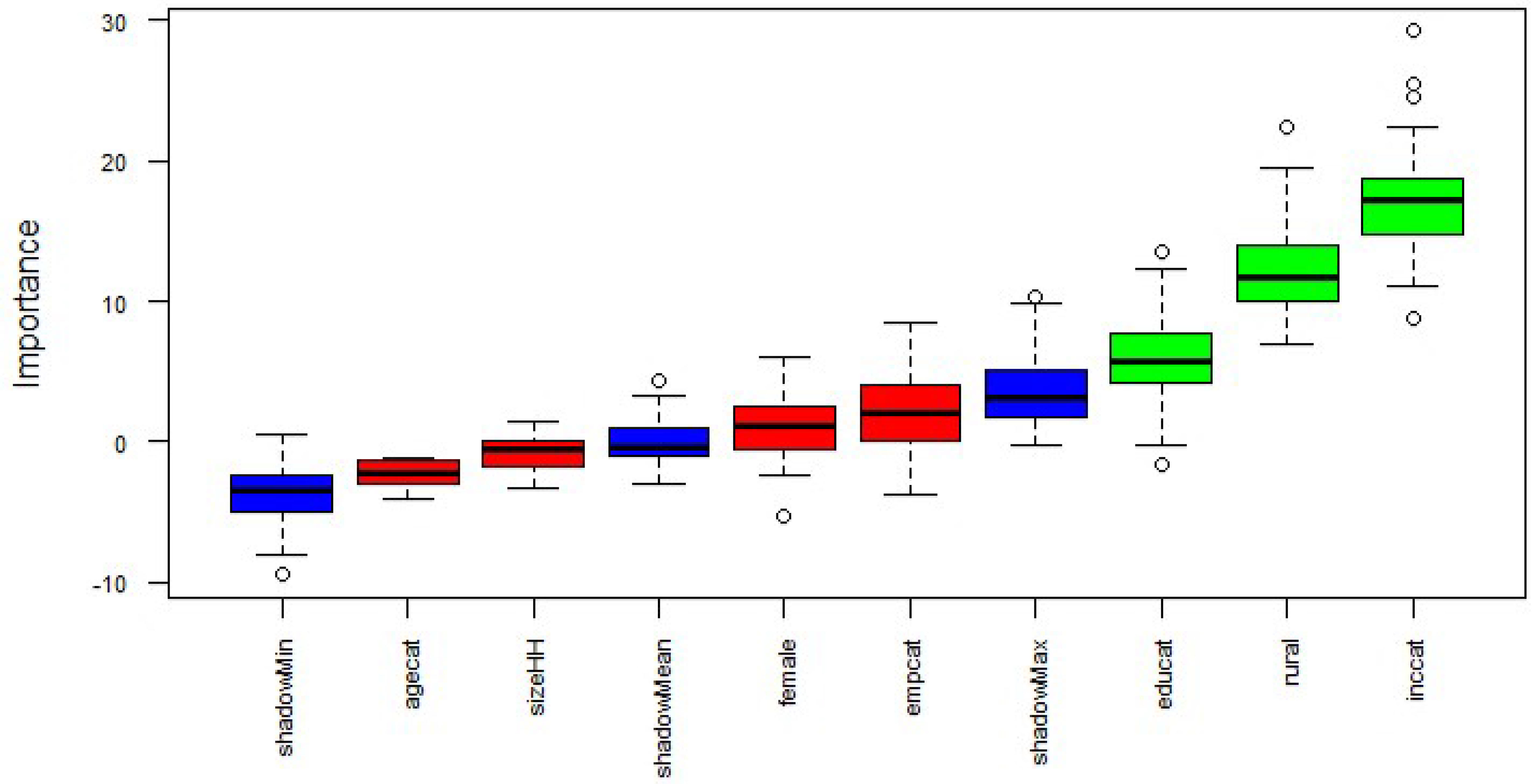
Figure 3.
Level of importance of the auxiliary variables for moderate or severe food insecurity.
3.3Steps for the implementation of the projection estimator
The main operational steps to implement the projection estimator can be summarized as follows:
1. Identifying and recoding auxiliary variables. The implementation of the projection estimator requires the availability of the same set of auxiliary variables in the two surveys to be integrated. These variables also need to share common structure and definitions.
2. Definition of the function
3. Computation of synthetic values. Using the estimated projection parameter, the synthetic values of the variable of interest are computed in the large dataset. This in turn, allows producing indirect disaggregated estimates of the indicator of interest.
4. Assessment of estimates accuracy. After producing synthetic estimates, their accuracy can be assessed estimating their variance, coefficient of variation and confidence intervals.
Step 1: Identifying and recoding auxiliary variables
Proper identification of the auxiliary variables
Despite the availability of a relatively small number of auxiliary variables common to the two datasets, this paper illustrates the use of the Boruta feature selection method, proposed in Kursa and Rudnicki [29], using a wrapper approach built around a random forest classifier [30]. In Boruta, the random forest used to fit the data follows a “greedy search” approach, i.e. it evaluates all the possible combinations of features against the established evaluation criterion (Mean Decrease Accuracy). In the process, Boruta iteratively compares the importance of each auxiliary variable against the importance of their shadow features, which are randomized versions of the original variables obtained by shuffling their values.
Figure 3 reports the output of the Boruta feature selection process, in which a series of boxplots in different colors represent the scores of the rejected (red – unimportant), tentative (yellow) and confirmed (green – important) auxiliary variables. The figure also shows, the shadow features (blue boxplots) identified by the algorithm. Tentative variables are those for which the Boruta feature selection method could not indicate a clear decision concerning their relevance, as their importance level was not significantly different from their best shadow feature.
All the levels of auxiliary variables identified as important by Boruta have been used to fit a logistic regression on the probability of being moderately or severely food insecure. In addition, all the relevant dimensions for data disaggregation (sex, age, income, rural/urban) are included in the regression model, in order to increase the unbiasedness of the projection domain estimator.
Step 2: Definition of the function
Let us indicate with
This choice allowed estimating the projection parameters
Table 5
Projected versus direct estimates of the probability of being moderately or severely food insecure (prob.ms). Estimates, Coefficients of variation (CV), and lower (L_CI) and upper (U_CI) bounds of 95% confidence intervals
| prob.ms | CV (%) | L_CI | U_CI | ||
|---|---|---|---|---|---|
|
IHS4 | Total | 0.91 | 1.2 | 0.89 | 0.93 |
|
GWP | 0.91 | 1.3 | 0.89 | 0.93 | |
| IHS4 | Female | 0.91 | 1.4 | 0.88 | 0.93 |
| GWP | 0.90 | 1.5 | 0.89 | 0.94 | |
| IHS4 | Male | 0.91 | 1.9 | 0.87 | 0.94 |
| GWP | 0.91 | 2.0 | 0.87 | 0.94 | |
| IHS4 | Rural | 0.93 | 1.2 | 0.90 | 0.95 |
| GWP | 0.92 | 1.3 | 0.90 | 0.94 | |
| IHS4 | Urban | 0.81 | 5.7 | 0.73 | 0.92 |
| GWP | 0.82 | 5.9 | 0.74 | 0.93 | |
| IHS4 | 15–24 | 0.91 | 2.0 | 0.87 | 0.94 |
| GWP | 0.89 | 2.1 | 0.85 | 0.93 | |
| IHS4 | 25–49 | 0.91 | 1.6 | 0.88 | 0.93 |
| GWP | 0.92 | 1.6 | 0.89 | 0.95 | |
| IHS4 | 50–64 | 0.87 | 3.6 | 0.82 | 0.94 |
| GWP | 0.90 | 3.5 | 0.84 | 0.96 | |
| IHS4 |
65 | 0.97 | 1.6 | 0.94 | 1.0 |
| GWP | 0.98 | 1.7 | 0.95 | 1.0 | |
| IHS4 | Inc_1 | 0.96 | 1.5 | 0.94 | 0.99 |
| GWP | 0.97 | 1.5 | 0.94 | 1.0 | |
| IHS4 | Inc_2 | 0.96 | 1.5 | 0.93 | 0.99 |
| GWP | 0.96 | 1.6 | 0.93 | 0.99 | |
| IHS4 | Inc_3 | 0.97 | 1.1 | 0.95 | 0.99 |
| GWP | 0.97 | 1.1 | 0.95 | 0.99 | |
| IHS4 | Inc_4 | 0.89 | 3.6 | 0.82 | 0.95 |
| GWP | 0.88 | 3.7 | 0.82 | 0.94 | |
| IHS4 | Inc_5 | 0.74 | 3.8 | 0.68 | 0.80 |
| GWP | 0.76 | 3.8 | 0.71 | 0.82 |
Then, the
with
Step 3: Computing the synthetic values in the large sample
Having obtained the estimates
Using the
for the total in the target population, and
for the proportion in the target population.
After fitting the working model, their assumptions and performance were assessed. A common approach adopted to deal with binary responses is the Hosmer and Lemeshow’s goodness of fit test [31]. According to this method, the model fits well when there is no significant difference between the model and the observed data (i.e. the
Step 4: Disaggregated estimates and the assessment of their accuracy
Estimates, standard errors and confidence intervals have been calculated for the relevant disaggregation dimensions (e.g. by sex, age, income and urban/rural area). The main empirical results are presented in Table 5. The comparison of projected versus direct estimates in terms of their coefficient of variation (CV) and Confidence Intervals (CI) shows that the former has a better (or at least equal) accuracy than the latter in almost all cases.
4.Conclusions and recommendations
After proposing an holistic approach to address data disaggregation, this paper provides a review of alternative methods for producing disaggregated estimates of SDG indicators having sample surveys as their primary data source. In particular, the article discusses methods to produce direct and indirect disaggregated estimates of SDG indicators and presents an empirical case study based on an extension of the projection estimator [2].
When addressing data disaggregation at the design stage, weighting sample-domain data allows computing direct domain-sampling estimates. In this context, the direct estimation of a parameter of interest is only possible when a sufficient number of sampling units is available in each disaggregation domain. Sampling designs for data disaggregation should ensure a planned sample size for each disaggregation domain included in the disaggregation plan. This action, on one hand, allows the computation of direct estimates, and on the other, support the production of more accurate indirect estimates by substantially reducing their bias. The article reviews various approaches that survey statisticians can rely on to improve sampling designs for data disaggregation. Traditional sampling techniques address this topic by leveraging oversampling, screening or a deeper stratification. However, these solutions may be too costly and difficult to implement in practical circumstances. New sampling approaches (such as marginal stratification sampling, indirect sampling or multisource sampling) allow for some of the abovementioned problems to be overcome without excessively increasing survey costs. They also enable sampling of rare or hard-to-reach populations.
With respect to data disaggregation at the analysis stage, the herein discussed model-assisted indirect estimation approach allows several interesting and relevant empirical applications for the production of disaggregated data for SDG (and other) indicators. In particular, most countries can normally rely on auxiliary variables provided by large-scale surveys, censuses, administrative records, or geospatial information. In this context, some of the target phenomena for SDG monitoring and data disaggregation are often too costly or complex to be incorporated in large-scale data collection campaigns. The approach described in this paper, based on an extension of the approach proposed in [2], allows measuring the variable of interest with a small-scale survey, by using the parameters of a regression-type working model that links this variable to a set of auxiliary variables. Based on these parameters, the values of the target variable can be predicted on a larger-scale data source collecting the auxiliary information used to fit the model. Reliance on a larger sample helps increase the accuracy of the disaggregated estimates and allows considering disaggregation domains that are not available in the small survey. In addition, predicting a variable of interest on the sample of a more extensive survey from which most national official statistics are produced, allows improving estimates’ consistency. Being a model-assisted approach, despite a good model fitting would allow increasing estimates efficiency, the proposed method is robust to wrong specifications of the model. Finally, it is also important to highlight that the proposed strategy could be easily extended to other empirical contexts where, instead of integrating two independent surveys, the small survey could be integrated with auxiliary information coming from other types of data sources, such as censuses, administrative registers, and/or earth observation data.
Notes
1 The term “indirect” estimation refers to completely different strategies and approaches than those related to “indirect” sampling methods discussed in Section 2.2.2. Indirect sampling methods are designed to plan and draw samples for a given target population, relying on the links that its units share with those of another population for which a good sampling frame is available.
2 In 2014, the FAO started collaborating with the Gallup Inc. to implement the FIES module in over 150 countries.
3 Initially, the dependent variables were grouped into three categories and an ordinal regression model was implemented. However, the greater complexity of the estimation approach was not compensated by a significant improvement of the performance of the model.
References
[1] | FAO. Guidelines on data disaggregation for SDG Indicators using survey data. Rome; Italy; (2021) . |
[2] | Kim JK, Rao JNK. Combining data from two independent surveys: A model-assisted approach. Biometrika. (2012) ; 99: (1): 85–100. |
[3] | Kalton G. Methods for oversampling rare subpopulations in social surveys. Survey Methodology. (2009) ; 35: (2): 125–142. |
[4] | Grafström A, Lundström NLP, Schelin L. Spatially balanced sampling through the pivotal method. Biometrics. (2012) ; 68: (2): 514–520. |
[5] | Kish L. Statistical Design for Research. John Wiley & Sons; New York City; USA; (1987) . |
[6] | Tourangeau R, Edwards B, Johnson TP, Wolter KM, Battese N. Hard-to-survey populations. Cambridge University Press; (2014) . |
[7] | FAO. Guidelines for enumeration of nomadic and semi-nomadic livestock. Rome; Italy; (2016) . |
[8] | FAO. Technical Report on the Integrated Survey Framework. Global Strategy to Improve Agriculture and Rural Statistics; Technical Report Series GO-02-2014; Rome; Italy; (2014) . |
[9] | FAO. Guidelines on the Integrated Survey Framework. Rome; Italy; (2015) . |
[10] | Lavallée P. Indirect Sampling. Springer; New York City; USA; (2007) . |
[11] | Singh AC, Mecatti F. Generalized multiplicity-adjusted horvitz-thompson estimation as a unified approach to multiple frame surveys. Journal of Official Statistics. (2011) ; 27: (4): 633–650. |
[12] | Falorsi PD, Righi P. Generalized framework for defining the optimal inclusion probabilities of one-stage sampling designs for multivariate and multi-domain surveys. Survey Methodology. (2015) ; 41: (1): 215–236. |
[13] | Falorsi PD, Righi P, Lavallée P. Cost optimal sampling for the integrated observation of different populations. Survey Methodology. (2019) ; 45: (3): 485–511; Statistics Canada; Catalogue No. 12-001-X. |
[14] | Cochran WG. Sampling Techniques. Wiley; New-York; (1977) . |
[15] | Jessen RJ. Statistical Survey Techniques. John Wiley & Sons; New York City; USA; (1978) . |
[16] | Lu W, Sitter RR. Multi-way stratification by linear programming made practical. Survey Methodology. (2002) ; 2: : 199–207. |
[17] | Tillé Y. Sampling and estimation from finite populations. John Wiley & Sons; (2020) . |
[18] | Deville JC, Tillé Y. Variance approximation under balanced sampling. Journal of Statistical Planning and Inference. (2005) ; 128: : 569–591. |
[19] | Chauvet G, Tillé Y. A fast algorithm for balanced sampling. Computational Statistics. (2006) ; 21: : 53–62. |
[20] | European Union Agency for Fundamental Rights. Second European Union Minorities and Discrimination Survey; Technical Report; EU-MIDIS II; Luxembourg; (2017) . |
[21] | Mecatti F. A single frame multiplicity estimator for multiple frame surveys. Survey Methodology, Statistics Canada, Catalogue No. 12-001-X, 33: (2): 151–157. |
[22] | Birnbaum ZW, Sirken MG. Design of sample surveys to estimate the prevalence of rare diseases: Three unbiased estimates. Vital Health Statistics. (1965) ; 2: (11): 1–8. |
[23] | Lavallée P. Cross-sectional weighting of longitudinal surveys of individuals and households using the weight share method. Survey Methodology. (1995) ; 21: (1): 25–32. |
[24] | Woodruff RS. A simple method for approximating the variance of a complicated estimate. Journal of the American Statistical Association. (1971) ; 66: (334): 411–414. |
[25] | FAO Sustainable Development Goals Webpage (available in Arabic, Chinese, English, French and Russian): https://www.fao.org/sustainable-development-goals/indicators/en/. |
[26] | Smith MD, Rabbitt MP, Coleman-Jensen A. Who are the world’s food insecure? New evidence from the food and agriculture organization’s food insecurity experience scale. World Development. (2017) ; 93: : 402–412. |
[27] | Ryan TP. Modern Regression Methods. Second edition. Wiley Series in Probability and Statistics; New York City; USA; John Wiley & Sons Book Series; (2008) . |
[28] | Harrell JFE. Describing, Resampling, Validating, and Simplifying the Model. Regression Modelling Strategies; Springer Series in Statistics; Switzerland; Springer International Publishing, (2015) ; 103–126. |
[29] | Kursa M, Rudnicki W. Feature selection with the boruta package. Journal of Statistical Software. September (2010) ; 36: (Issue 11). |
[30] | Breiman L. Random forests. Machine Learning. (2015) ; 45: (1): 5–32. |
[31] | Hosmer DW, Lemeshow S, Sturdivant RX. Applied Logistic Regression. Third edition. Wiley Series in Probability and Statistics. (2013) . |
[32] | Archer K, Lemeshow S, Hosmer DW. Goodness-of-fit test for logistic regression models when data are collected using a complex sample design. Computational Statistics & Data Analysis. (2007) ; 51: (9): 4450–4464. |

