
The use of combined Landsat and Radarsat data for urban ecosystem accounting in Canada
Abstract
This paper describes an approach for combining Landsat and Radarsat satellite images to generate national statistics for urban ecosystem accounting. These accounts will inform policy related to the development of mitigation measures for climatic and hydrologic events in Canada. Milton, Ontario was used as a test case for the development of an approach identifying urban ecosystem types and assessing change from 2001 to 2019. Methods included decomposition of Radarsat images into polarimetric parameters to test their usefulness in characterizing urban areas. Geographic object-based image analysis (GEOBIA) was used to identify urban ecosystem types following an existing classification of local climate zones. Three supervised classifiers: decision tree, random forest and support vector machine, were compared for their accuracy in mapping urban ecosystems. Ancillary geospatial datasets on roads, buildings, and Landsat-based vegetation were used to better characterize individual ecosystem assets. Change detection focused on the occurrence of changes that can impact ecosystem service supply – i.e., conversions from less to more built-up urban types. Results demonstrate that combining Radarsat polarimetric parameters with the Landsat images improved urban characterization using the GEOBIA random forest classifier. This approach for mapping urban ecosystem types provides a practical method for measuring and monitoring changes in urban areas.
1.Introduction
Urban areas are among the most complex manifestations of man’s impact on the environment [1]. They consist of a wide array of heterogeneous materials with diverse properties and multi-faceted interactions. Combinations of buildings (e.g., low- and high-rises), impervious surface covers (e.g., roads and parking lots), vegetation (e.g., parks and sports fields), bare soil (empty lots and unattended garden plots) and water (e.g., wetlands and streams) are fundamental components of the urban ecosystem [1, 2]. More research is needed on the impact of land conversion on ecosystem assets and services in urban areas, and on the resilience of urban areas to climate change given its pressures on ecosystems, both in Canada and elsewhere.
Statistics Canada is creating a suite of ecosystem accounts that link environmental information to socio-economic data available in the System of National Accounts and elsewhere in the national statistical system. These ecosystem accounts will contain information on both the quantity and quality of ecosystem assets and their services, in both physical and eventually, monetary terms. The System of Environmental – Economic Accounting – Experimental Ecosystem Accounting (SEEA-EEA) provides guidelines for compiling ecosystem accounts [3].
Considering the large and growing proportion of the world population living in cities, with 68% of the world population projected to live in urban areas by 2050 [4], an emerging interest concerns ecosystem accounting for urban areas. Urban areas can be considered a specific category of ecosystem, or can alternatively be understood as a combination of multiple ecosystem types.11 In both cases, urban areas produce and benefit from ecosystem services.
Statistics Canada has already developed statistical data and analysis for urban areas by integrating maps generated from satellite Earth observation (EO) data and socio-economic data to provide new insights on urban expansion and natural and semi-natural ecosystems impacted by changes in the landscape surrounding metropolitan areas [5]. This analysis made use of geospatial datasets produced by other federal departments, including Agriculture and Agri-Food Canada [6, 7] and Natural Resources Canada [8]. These datasets, although of high quality, were produced to meet the mandates and needs of those departments for tracking cropland and forests. However, they do not provide the precision needed to delineate urban areas as a specific ecosystem type that combines impervious surface, buildings, vegetation and water or to delineate intra-urban level ecosystem assets. As such, they do not meet the ‘fit for purpose’ criteria required of spatial datasets for more focused urban ecosystem accounting.
In 2018, Statistics Canada and the Canadian Space Agency (CSA) signed an agreement, under the CSA’s Government Initiatives Related Program (GRIP), to collaborate on the improvement of urban delineation and characterization in the context of Climate Change Impacts and Ecosystem Resilience (CCIER). The Earth Observation for Ecosystem Accounting in Canada (EO4EA-Can) project aims to integrate earth observation data with socio-economic information to better measure the climate change resilience of built-up areas in the context of ecosystem accounting. The main objective of this project is to map urban areas, including both the built-up structures and ‘green and blue infrastructure,’ and assess the changes in the extent and density of these types of assets, using optical and radar imagery, complemented with census and geospatial data. Green and blue ecosystem assets are of specific policy interest in urban areas since they provide ecosystem services that can improve human health and well-being and buffer against natural disturbances and extreme weather events. Maintaining these services may have a crucial role in increasing adaptive capacity to cope with climate change [9].
This case study on the integration of Landsat and Radarsat for urban ecosystem accounting is a first step towards this larger objective. Milton, Ontario has been used as a test case and subsequent test cases are being developed in other regions of the country. The development of better spatial data to support urban ecosystem accounting will help inform policy and investment decisions related, for example, to the identification and development of mitigation measures for climatic and hydrologic impacts (i.e., those relating to urban heat islands and energy consumption, air pollution, increased runoff, modified streamflow dynamics, or water quality) at a regional scale across the country; and in this way will contribute to the health, security and well-being of Canadians.
2.Background
The delineation and characterization of areas into a complete set of mutually exclusive and contiguous spatial units is at the foundation of ecosystem accounting. The Technical Recommendations of the SEEA-EEA [3] defines three main spatial units relevant to the production of accounts: 1) ecosystem assets, 2) ecosystem types and 3) ecosystem accounting areas. A basic spatial unit is additionally described in the recommendations; it represents fine-scaled gridded cells or polygons that underlie the delineation of ecosystem assets.
In ecosystem accounting, stocks of ecosystem assets generate flows of ecosystem services. Individual ecosystem assets can be grouped according to ecosystem types (e.g., forest, wetland, cropland, urban) that are expected to generate a similar bundle of ecosystem services [3]. Typically, ecosystem accounts are compiled and presented by ecosystem type rather than by individual ecosystem asset and they may be reported for different ecosystem accounting areas (e.g., at a national or sub-national level or for a specific ecosystem type (e.g., forest or urban). Thus, a classification describing the ecosystem types and a map showing their occurrences are essential components of ecosystem accounting that allow tracking changes over time.
If spatial data on ecological characteristics are not available to delineate the ecosystem assets, a land cover map may be used as a starting point [3]. Land cover can be defined as the “observed (bio) physical cover of the Earth’s surface,” [10] and is a synthesis of the many processes taking place on the land. It reflects land occupation by various natural, modified or artificial systems. Land cover is one of the most easily detectable indicators of human intervention on land [10].
2.1Urban characterization for ecosystem accounting
Urban ecosystem accounting has considered the use of different levels of detail in the delineation of urban ecosystem assets and types – from the detailed level of the individual green assets, such as rows of street trees or green roofs, to larger patches of urban area with common characteristics to which ecosystem services can be attributed. The focus, in this study, is this latter perspective: analyzing urban morphological structure at the landscape level to define urban ecosystem types. The challenge in doing so lies in the spectral complexity of the urban environment [11]. The urban environment is composed of various natural (e.g., vegetation, bare soil, bare rock and sand) and artificial features (e.g., buildings, roads and urban open space) constructed with different kinds of materials. Many natural surfaces are spectrally similar to the artificial features. Remote sensing analysis should therefore consider not only the spectral characteristics of different materials, but also contextual information [2].
Assessing the ecosystem services generated by urban ecosystem types at landscape level requires that urban areas be subdivided into smaller patches that maintain structural diversity while being regrouped within homogeneous areas [12]. For example, urban heat island studies have developed local climate zones (LCZs), a generic, climate-based typology of urban and natural landscapes that integrates surface structure (height and density of buildings and trees) and surface cover (pervious or impervious) [13]. The classes are local in scale, climatic in nature, and zonal in representation. LCZs are defined as “regions of uniform surface cover, structure, material, and human activity that span hundreds of meters to several kilometres in horizontal scale” and have a “characteristic screen-height temperature regime” [13]. The physical properties of all zones are measurable and nonspecific as to place or time. A generic urban classification scheme, which addresses the constructional characteristics of a surface (i.e., the land cover and not the usage), facilitates the classification of urban land cover into classes representing real world features with an organized system that enables the comparison between urban classes and their components [2].
The Stewart and Oke LCZs classification consists of 17 standard classes, of which 15 are defined by surface structure and cover, and two by construction materials and anthropogenic heat emissions [13].
2.2Earth observation sensors
Satellite earth observation uses remote-sensing technologies including optical, infrared and radar sensors to collect information about physical and other characteristics of the Earth, such as land cover, vegetation, temperature and aerosols. The choice of sensors for the identification of detailed urban ecosystem types should consider and balance between the sensor’s technical characteristics such as spatial, spectral, radiometric and temporal resolution, and feasibility, so that the resulting data are of sufficient quality and are useful for ecosystem accounting. Desirable characteristics include high to very high spatial resolution; good coverage of the electromagnetic spectrum, including number and width of spectral bands; radiometric accuracy and reliability (radiometric resolution is determined by the sensitivity to the magnitude of the electromagnetic energy e.g. 8, 16, 32 bits); and suitable temporal scales, including historical coverage and revisit times. These characteristics will also have an impact on the practicality and efficiency of the processing.
The Landsat series22 satellites are the most common optical Earth observation (EO) data sources for land cover mapping, including for urban, peri-urban and rural areas [14]. Zhang et al. described Landsat data as efficient and cost effective for mapping urban areas in Canada [15]. This is particularly relevant for a large country like Canada, where population centres – areas with a population of at least 1,000 and a population density of 400 persons or more per square kilometre [16] – cover an area of approximately 18,000 km2 (or 1.5% of Canada landmass), distributed across the 1,210,519 km2 (or 12% of Canada landmass) that correspond to the 2016 population ecumene [17].
The Landsat series provides nearly continuous coverage since the early 1970s. Landsat-8 is the latest satellite in the series, providing imagery since 2013. The seven spectral bands (multispectral) at a spatial resolution of 30 m, coupled with the 15 m visible band (panchromatic), offer sufficient spatial and spectral information to map major urban land use classes, such as residential, recreational and industrial/commercial/institutional. Another benefit is that the United States Geological Survey (USGS) provides analysis ready data (ARD) for Landsat 4–8, resulting in a highly accurate surface reflectance image, which significantly reduces the pre-processing required by users [14].
The Global Human Settlement Layer (GHSL) produced by the Joint Research Centre (JRC) of the European Commission, used Landsat data for mapping built-up areas worldwide. These datasets contain a multi-temporal information layer of built-up presence derived from Landsat image collections from 1975 to 2014 [18, 19, 20]. The GHSL-built dataset was combined with a population grid to produce the degree of urbanisation. The degree of urbanisation is described by the classes: 1) cities, 2) towns and suburbs, and 3) rural areas [21, 22]. However, a preliminary review of the accuracy of the GHSL built-up area in Canada has identified some issues [5]. In some cases, the product struggles to accurately delimit the urban extent or cannot differentiate the urban landscape into separate urban classes. However, although GHLS overestimates the area of settlements in some places and does not capture the built-up area in others, it remains a useful tool as a basis for change analysis and comparison of built-up areas.
The Sentinel-2 satellites from the European Space Agency (ESA) Copernicus programme can be used to complement Landsat-8 imagery for urban area mapping and monitoring [22, 23], although the satellites (A and B) were only launched recently (2015 and 2017) reducing the capacity to do historical comparisons. The twin satellites have 13 spectral bands, with spatial resolution of 10 m, 20 m and 60 m in the visible, near infrared and shortwave infrared bands of the electromagnetic spectrum. They offer a revisit time of five days.
Very high resolution images (< 5 m) can map detailed urban features and can therefore provide useful additional information to understand the heterogeneity of urban areas that is not otherwise available using Landsat or Sentinel. However, such datasets are costly and they require a more significant use of computing resources for analysis compared to Landsat data, especially when covering a large area. Also, with very high resolution images, the heterogeneity of urban areas is amplified by the illumination of surfaces exposed to the sun and the resulting shadows create noise in the signal measured on the image [24].
Synthetic aperture radar (SAR) has been recognized as an effective tool for urban analysis, as it is less influenced by solar illumination or weather conditions (e.g., cloud cover) compared to optical or infrared sensors [25]. SAR sensors can acquire information in different polarizations (these are related to the orientation of the electromagnetic field), which helps provide a more complete description of the target. SAR data have been increasingly used for urban land use and land cover (LULC) classification [26, 27, 28]. The difficulty in detailed urban mapping using SAR data is mainly due to the complexity of the urban environment – its many different kinds of natural and built objects and materials, orientations, shapes, sizes, etc. complicate the interpretation of SAR images [25, 29, 30, 31].
The integration of optical and polarimetric SAR data is seen as a promising approach to improve urban impervious surface mapping [29, 32], because it helps resolve issues with the diversity of urban land covers and the spectral overlap between covers. The Global Urban Footprint (GUF) project from the German Aerospace Agency (DLR) demonstrated that SAR data can be used with optical data to delineate urban areas. SAR data usefully captures built environments, since these exhibit strong scattering properties as a result of double bounce effects and direct backscattering from vertical building structures [33, 34, 35, 36]. The GUF project, like most studies about urban mapping using SAR data was, however, limited to the identification of the urban extent and relative built-up density.
The approach developed by DLR for mapping urban areas using Sentinel-1 data (SAR) has also been tested with success on Radarsat-2 images [37]. In addition, previous comparative studies on the combined use of multispectral optical and polarization SAR data to identify urban areas have demonstrated that polarization data improved the accuracy of results [28, 38, 39].
The Canadian Radarsat-2 https://mdacorporation. com/geospatial/international/satellites/RADARSAT-2/ satellite has a C-band synthetic aperture radar (SAR) with multiple polarization modes, including a fully polarimetric mode in which HH, HV, VV and VH polarized data are acquired. The spatial resolutions range from 1 m to 100 m. The radar signal in different polarizations determines physical properties of the observed object and the use of polarimetric parameters can provide a more complete characterization of the target. Polarimetric target decomposition has become the standard method for the extraction of parameters from polarimetric SAR data [39]. Once decomposed, the physical properties of the target are extracted and interpreted through the analysis of the simpler responses [31, 40, 41, 42].
Touzi multiresolution decomposition is a method that considers the target’s structure to generate the decomposition [41, 43]. It uses a scattering-vector model to represent each coherency eigenvector in terms of unique target characteristics. Each coherency eigenvector is uniquely characterized by five independent parameters. Scattering type is described with a complex entity, whose magnitude (alpha_s) and phase (phi) characterize the magnitude and phase of target scattering. The helicity (tau) characterizes the symmetric-asymmetric nature of the target scattering. The angle (psi) is the target orientation. To complement the decomposition, discriminators can be used to provide the intensity of the target’s response. The algorithm developed by Touzi [40] derives the maximum and minimum degrees of polarization and total intensity of the scattered wave. Touzi decomposition and discriminators have been shown to provide better classification for urban areas with high variability and complexity, compared to other decomposition methods [31].
2.3Classification approach
Depending on the resolution of the data provided by the sensor, pixels may contain more than one type of land cover. This is particularly a problem in heterogeneous areas like cities, where a given 30 m pixel may contain built structures, impervious surfaces, and different types of vegetation [11]. Conventional pixel-based classifiers, such as maximum likelihood classification (MLC), cannot effectively handle the mixed-pixel problem in urban areas. In the MLC classification, the distribution of each class is assumed to come from a normal distribution. The probability that a given pixel belongs to a specific class is calculated using the mean vector and the covariance matrix. Each pixel is then assigned to the class that has the highest probability (the maximum likelihood) [11].
Moreover, in the pixel-based approach, the proportion of the signal coming from the surrounding area is ignored. Alternative approaches that use geographic object-based image analysis (GEOBIA) with machine learning classifiers provide better results [24].
The GEOBIA approach provides a geographic information system-like functionality for classification that integrates not only the spectral but the spatial characteristics during the image segmentation process. The result is individual areas with shape and spectral homogeneity referred to as segments or objects [44]. This method can make use of varied data sources including multi-sensors, geospatial datasets and any spatially-distributed variable (elevation, slope, population density) [11]. GEOBIA uses a two-step approach. First, the segmentation process defines homogeneous objects and second, classifies these objects into a classification scheme based on spectral, spatial and contextual information. Objects are assigned to land cover classes representing real-world features (e.g., open low-rise, compact medium-rise, sparsely built, dense trees, and paved), instead of a somewhat arbitrary pixel structure [45]. Object-based methods, which make use of contextual information to improve mapping accuracy, are increasingly employed [11, 29, 46].
A comparison of pixel-based and object-based approaches for identifying urban land-cover classes has demonstrated that the object-based classifier produced a significantly higher overall accuracy. In addition, segmentation procedures used in GEOBIA can be applied following a hierarchical structure where classes are defined at an appropriate scale [29, 47].
Nonparametric classification approaches using machine learning algorithms such as artificial neural network, decision tree (DT), random forest (RF) and support vector machine (SVM) are widely used in land cover classification [30, 46]. Niu, X. and Y. Ban used the object-based SVM for the classification of Radarsat-2 polarimetric parameters in order to produce an urban land cover classification [30]. The results showed that SVM can map detailed urban land cover classes with high accuracy (90%); it provides homogeneous mapping results with preserved shape details; and outperforms other land cover classification approaches in a complex urban environment with limited training samples [30].
Machine learning classifiers were used to map seven land cover classes in the United Kingdom with Landsat data [48]. Results from this study suggest that the RF classifier performs equally well to SVM in terms of classification accuracy and training time. This study also concluded that fewer user-defined parameters are required by the RF classifier than for SVM and that they are easier to define. However, the performance of the classifiers was highly dependent upon several factors such as the training set design (i.e., sample selection, composition, purity and size), even though the nonparametric algorithm does not require normally distributed training data [11], as well as input imagery resolution and landscape heterogeneity [49].
Finally, other studies have demonstrated that the integration of indices such as Normalized Difference Vegetation Index (NDVI) and Normalized Difference Water Index (NDWI) into the segmentation and classification processes can improve the results for urban characterization [50, 51].
2.4Change detection
Images acquired on different dates rarely capture the landscape surface in the same way due to many factors including illumination conditions, view angles and meteorological conditions [52]. Change detection methods that use the pixel as the change unit are negatively affected by these factors. Problems with pixel change detection are usually caused by the complexity of change conditions such as small spurious changes, the accuracy of image registration, and shadows resulting from different viewing angles, which can be dominant in urban areas. Pixel-level comparison for change detection therefore requires further analysis to attach a meaning to the change observed [53]; for example, to assess a decrease of forest canopy, a geospatial analysis is required to define forest patches. By contrast, the GEOBIA approach transforms spectral and spatial properties of the image into meaningful objects, thereby creating features that have real-world meaning (e.g., buildings) [52, 53]. Object-based change detection reduces the problems associated with assessing pixel-level changes.
Object-based analysis offers great potential for identifying and characterizing LULC change processes, especially when combined with multi-temporal analysis. Segmentation-generated objects from different dates often vary geometrically, even though they represent the same geographic features. Instead of separately segmenting these images, the use of multi-temporal object change detection takes advantage of all multi-temporal states of the scene [54]. Specifically, temporally sequential images are combined and segmented together, producing spatially corresponding change objects [52]. For example, Schneider et al. used the NDVI generated from Landsat time series from 1985 to 2015 to detect urban extents, identify the conversion types and the date the change occurred [55].
3.Methods
In support of the creation of detailed urban maps for ecosystem accounting, the objective of this case study was to develop a classification approach to improve the accuracy of urban land cover maps generated from Radarsat-2 and Landsat Operational Land Imager (OLI) observations at 30 m. This paper describes both the mapping approach using machine learning classifiers applied on Radarsat-2 polarimetric parameters and the characteristics of the produced map.
3.1Study area
Milton is a town located in Southern Ontario, Canada, and is part of the Toronto census metropolitan area. Between 2001 and 2011, Milton was the fastest growing municipality in Canada, with a 71.4% increase in population from 2001 to 2006, and another 56.5% increase from 2006 to 2011. In 2016, Milton’s population was 110,128 and it is forecasted to grow to 228,000 by 2031 [56]. While most of the development is suburban in nature, larger industrial lots are being developed, and commercial and institutional facilities have been built as well. The built-up patterns in Milton are fairly representative of suburban growth within the Toronto CMA, which represents 44% of the population of Ontario and 17% of the total population of the country.
3.2Satellite data and pre-processing
Radarsat-2 fine quad pol wide images33 in different angles were acquired for Milton for the months of July to October 2019 to test the multi-polarization information. All images were converted in Sigma Nought format and then orthorectified. The pixel size of all images, even if they were acquired in different angles, was resampled at 8 m for better comparison. A Lee adaptive filter with a window of 7 by 7 was applied on the images to reduce the speckle effect [57]. The Touzi multiresolution decomposition [41] was performed using Geomatica software [57] and created an image of 15 decomposition parameters. For each of the primary, secondary, and tertiary eigenvectors, the orientation angle (psi), dominant eigenvalue (lambda), alpha_s angle, phase, and helicity (tau) are computed.
These parameters characterize the properties of scattering by computing the proportion and type of the scattering mechanism for all features in the image. For example, the Alpha S polarimetric parameter measures the double bounce response resulting from the interaction of the radar signal with a corner reflector created by two or more smooth, flat surfaces oriented at a 90-degree angle to each other (most commonly an impervious surface and a building). Four Touzi discriminators [40] were also generated for measuring the intensity of the signal returned to the sensor [57]. The computed discriminators include the Touzi anisotropy, the degrees of minimum and maximum polarization response, and the difference between the maximum and minimum response. Table 1 provides the list of the parameters used for the assessment.
Table 1
List of Radarsat-2 polarimetric parameters
| Touzi decomposition | |
|---|---|
| Difference between Max and Min Response | |
| Touzi Anisotropy | |
| Minimum Polarization Response | |
| Maximum Polarization Response | |
| Touzi discriminators | |
| Eigenvectors | Parameters |
| Dominant | Psi Angle |
| Eigenvalue (Lambda) | |
| Alpha S Parameter | |
| Phase | |
| Tau Angle (Helicity) | |
| Secondary | Psi Angle |
| Eigenvalue (Lambda) | |
| Alpha S Parameter | |
| Phase | |
| Tau Angle (Helicity) | |
| Tertiary | Psi Angle |
| Eigenvalue (Lambda) | |
| Alpha S Parameter | |
| Phase | |
| Tau Angle (Helicity) | |
Landsat analysis ready data (ARD) images were selected from the USGS Earth Explorer platform portal for census years 2001, 2006, 2011, and 2016. Imagery was also downloaded for the most recent year (2019) to have the most up-to-date classification possible. Multiple images were downloaded for each year to cover seasonal variability from spring to fall. The NDVI was calculated for each image.
3.3Training and validation data selection and classification scheme
The 2016 Census of Population geographic boundary for the population centre of Milton [58] was used to delineate the urban core and buffered by an arbitrary distance of two kilometres to include the newly built-up areas in the peri-urban area. A buffer distance of two kilometres was found to capture the majority of new built-up areas that occurred outside of the population centre between 2016 and 2019. The 2019 Radarsat-2, Landsat ARD and the buffered population centre polygon for Milton were loaded into a project using the commercial software eCognition V9.4.44 A multiresolution segmentation, based on the 2019 Landsat NDVI from spring, summer and fall, was generated to create meaningful objects, i.e., different urban ecosystem types. Identification of training classes was performed through visual interpretation of Landsat data and high resolution imagery available through Google Earth and on-site visits to assign a class to each polygon.
The approach used a classification scheme based on the local climate zone (LCZ) classes developed by Stewart and Oke for the urban ecosystem types (Table 2) [13]. For each LCZ class, 75% of the polygons were randomly selected for training. The remaining 25% were kept for validation. A total of 723 polygons were selected for training and 237 for validation (Table 3). This proportion was chosen to balance between what is statistically sound and what is practicably attainable.
Table 2
Description of local climate zone classes found in Milton, Ontario [13]
| Code | LCZ classes | Description of local climate zone (LCZ) classes |
|---|---|---|
| LCZ 3 | Compact low-rise | Dense mix of low-rise buildings (1–3 stories). Few or no trees. Land cover mostly paved. |
| LCZ 6 | Open low-rise | Open arrangement of low-rise buildings (1–3 stories). Abundance of pervious land cover (low plants, |
| scattered trees). | ||
| LCZ 8 | Large low-rise | Open arrangement of large low-rise buildings (1–3 stories). Few or no trees. Land cover mostly paved. |
| LCZ 9 | Sparsely built | Sparse arrangement of small or medium-sized buildings in a natural setting. Abundance of pervious land |
| cover (low plants, scattered trees). | ||
| LCZ A | Dense trees | Heavily wooded landscape of deciduous and/or evergreen trees. Land cover mostly pervious (low plants). |
| Zone function is natural forest, tree cultivation, or urban park. | ||
| LCZ B | Scattered trees | Lightly wooded landscape of deciduous and/or evergreen trees. Land cover mostly pervious (low plants). |
| Zone function is natural forest, tree cultivation, or urban park. | ||
| LCZ D | Low plants | Featureless landscape of grass or herbaceous plants/crops. Few or no trees. Zone function is natural |
| grassland, agriculture, or urban park. | ||
| LCZ E | Paved | Featureless landscape of rock or paved cover. Few or no trees or plants. Zone function is natural desert |
| (rock) or urban transportation. | ||
| LCZ F | Bare soil | Featureless landscape of soil or sand cover. Few or no trees or plants. Zone function is agriculture. |
| LCZ G | Water | Large, open water bodies such as seas and lakes, or small bodies such as rivers, reservoirs, and lagoons. |
Table 3
Number, area and average area of polygons used for training and validation per LCZ class
| Training objects | Validation objects | |||||
|---|---|---|---|---|---|---|
| LCZ | Count | Total area (km2) | Average area (km2) | Count | Total area (km2) | Average area (km2) |
| Bare soil | 51 | 4.37 | 0.09 | 16 | 1.31 | 0.08 |
| Compact low-rise | 18 | 8.82 | 0.49 | 6 | 1.86 | 0.31 |
| Dense trees | 34 | 5.23 | 0.15 | 11 | 1.58 | 0.14 |
| Large | ||||||
| Low-rise | 64 | 5.40 | 0.08 | 21 | 1.86 | 0.09 |
| Low plants | 283 | 32.88 | 0.12 | 94 | 11.52 | 0.12 |
| Open | ||||||
| Low-rise | 36 | 6.18 | 0.17 | 12 | 3.02 | 0.25 |
| Paved | 33 | 2.95 | 0.09 | 11 | 0.68 | 0.06 |
| Scattered trees | 63 | 7.40 | 0.12 | 20 | 1.71 | 0.09 |
| Sparsely built | 92 | 7.35 | 0.08 | 30 | 3.51 | 0.12 |
| Water | 49 | 0.71 | 0.01 | 16 | 0.16 | 0.01 |
3.4Object-based classification
The decision tree (DT), random forest (RF), and support vector machine (SVM) supervised classification models were evaluated. Each classifier was trained and validated, and the accuracy of each classification was compared. Radarsat-2 polarimetric parameters Alpha S, Dominant Lambda, Tertiary Lambda and Maximum Intensity, and Landsat spectral bands and NDVI were used to create classifier statistics from the same set of training samples. The accuracy of the three classifications was assessed using the same set of validation polygons.
3.5Ecosystem assets calculation
Urban ecosystem accounting requires the delineation of individual ecosystem assets that make up the entire fabric of urban areas (e.g., vegetation, buildings, impervious surface, bare soil and water).
The total area and the percentage of vegetation coverage by each LCZ class were calculated using a binary map of vegetation based on the NDVI from Landsat imagery. All available Landsat NDVI imagery was acquired for 2019 and the maximum NDVI value for each pixel was selected. A binary vegetation mask was generated by manually specifying a threshold for the maximum NDVI value observed for 2019.
The road coverage was derived from the Road Network File (RNF) from Statistics Canada, a digital representation of Canada’s national road network [59]. All road line features were buffered by four metres55 to create road polygons in order to calculate the road area of each LCZ class.
The building coverage was drawn from Microsoft’s Building footprint dataset [60] dated March 2019. This dataset includes the footprint of nearly 12 million buildings, covering all provinces and territories in Canada. The total area and percentage coverage of the building footprints were calculated for each LCZ class.
3.6Change detection
Object-based change detection analysis captures change by comparing the values of objects over several dates. The annual mean maximum NDVI values for 2001, 2006, 2011, and 2016 census years, and 2019, were compared to identify the type of landscape change and timing of its occurrence for each built-up image object from the 2019 segmentation. To calculate the annual maximum NDVI value for a given year, all available Landsat NDVI images were acquired and the highest NDVI value for each pixel was selected. The NDVI values within each built-up object were averaged to obtain the mean maximum NDVI value. Assessing the change directly from the NDVI value reduces the error introduced by post classification change analysis, where misregistration and misclassification can lead to false changes.
The Landsat-8 sensor acquires data in two thermal bands, in addition to the seven spectral bands. The USGS systematically processes the thermal bands to create a surface temperature product, which is available for all ARD image dates. A single surface temperature image was selected for each year of the analysis. The individual images were chosen to coincide with typical summer temperatures and with daily temperature readings from two nearby weather stations. Local surface temperature is dependent on a number of factors such as elevation, vegetation, topography, solar radiation and prevailing winds.
Surface temperature was calculated for each object by averaging the individual pixel values within the object. The maximum surface temperature value for each date, as measured at the weather stations, was then subtracted from the mean value of each object to adjust for differences between dates. The final surface temperature values for each object represent the deviation from the maximum surface temperature observed at the weather stations.
4.Results and discussion
Results show that the polarimetric parameters contributed to the classification of the local climate zone (LCZ) urban ecosystem types. The best result is obtained with the random forest (RF) algorithm, which had an overall accuracy of 74% and a kappa of 0.68 (note that a kappa value of 1 represents perfect agreement, while a value of 0 represents no agreement) (Table 4). The RF algorithm applied on the Landsat-8 combined with the Radarsat-2 image provided better results for most of the classes when compared to the Landsat-8 only classification (Table 5), for both the producer accuracy and user accuracy.
Table 4
Comparison of the overall accuracy for the classifications
| Classification | Overall accuracy | Kappa |
|---|---|---|
| Landsat-8 (DT) | 56.96% | 0.49 |
| Landsat-8 (RF) | 64.98% | 0.58 |
| Landsat-8 (SVM) | 54.85% | 0.42 |
| Landsat-8 and Radarsat-2 (DT) | 62.45% | 0.54 |
| Landsat-8 and Radarsat-2 (RF) | 74.26% | 0.68 |
| Landsat-8 and Radarsat-2 (SVM) | 55.70% | 0.43 |
Table 5
Comparison of the producer’s and user’s accuracy for Landsat-8 (L8) and Landsat-8 combined to Radarsat-2 (RS2) at class level (%)
| Classification | Accuracy | Water | Low plants | Dense trees | Scattered trees | Sparsely built | Bare soil | Paved | Large low-rise | Open low-rise | Compact low-rise |
|---|---|---|---|---|---|---|---|---|---|---|---|
| L8 (RF) | Producer | 94 | 59 | 100 | 45 | 73 | 81 | 18 | 76 | 58 | 67 |
| User | 100 | 90 | 85 | 43 | 44 | 57 | 17 | 89 | 47 | 44 | |
| L8-RS2 (RF) | Producer | 94 | 76 | 91 | 45 | 77 | 88 | 45 | 90 | 42 | 83 |
| User | 100 | 89 | 83 | 69 | 52 | 67 | 50 | 86 | 45 | 56 | |
| L8-RS2 (RF) | Omission | 6 | 24 | 9 | 55 | 23 | 12 | 55 | 10 | 58 | 17 |
| Commission | 0 | 11 | 17 | 31 | 48 | 33 | 50 | 14 | 55 | 44 |
Producer accuracy is the probability that a value in a given class was classified correctly from the point of view of the map maker. User accuracy is the probability that a value predicted to be in a certain class really is in that class. The probability is based on the fraction of correctly predicted values to the total number of values predicted to be in a class. For example, in Table 5, the producer accuracy for the ‘Compact low-rise’ class was 83% while the user accuracy was 56%. This means that even though 83% of the reference sites classified as Compact low-rise areas have been correctly identified as Compact low-rise, only 56% percent of the areas identified as Compact low-rise in the classification were actually Compact low-rise. The producer’s accuracy is a complement of the omission error, while the user’s accuracy is a complement of commission error. Errors of omission refer to reference sites that were left out (or omitted) from the correct class in the classified map. In the case of Compact low-rise, 17% of this class was omitted, while 44% of polygons identified as Compact low-rise were, in reality, other classes.
Polarimetric decomposition parameters can explain the target scattering mechanisms in different ways. However, their basic scattering mechanisms include three main classes: surface scattering, volume diffusion scattering and double bounce scattering. Table 6 explains the way in which polarimetric parameters contributed to the improvement of the classification of the LCZ urban type classes.
Table 6
Scattering mechanisms associated with the polarimetric parameter for each LCZ class
| Ranking RS2 contribution | LCZ | Scattering mechanisms | Polarimetric parameters |
|---|---|---|---|
| 1 | Paved | Surface | Lambda 1, maximum intensity |
| 2 | Compact low-rise | Double bounce and volume scatter | Alpha S, Lambda 3 |
| 3 | Bare soil | Surface | Lambda 1 |
| 4 | Sparsely built | Volume scatter | Lambda 3 |
| 5 | Scattered trees | Volume scatter | Lambda 3 |
| 6 | Low plants | Surface | Lambda 1 |
| 7 | Large low-rise | Double bounce | Alpha S |
The overall accuracy of the results of this approach may seem low compared to the literature, where a threshold of 85% is typically recognized as an acceptable level of accuracy [61]; however, the results should be analyzed at the class level. Moreover, even if the accuracy of one class is low, if it represents a green and blue ecosystem type that is important for defining ecosystem services, then this class can be conserved in the result. Nonetheless, the assessment of this class should be analyzed with ancillary data to avoid unacceptable errors.
Given that urban type class definitions from LCZs are based on a combination of structural and biophysical criteria observed on the ground, the use of remote sensing to map LCZs classes may introduce overlap between classes. However, this overlap can be explained when looking at the spectral response. For example, the accuracy of the ‘Paved’ class is low compared to the other classes (45% for producer accuracy and 50% for user accuracy) because of its confusion with other built-up classes that have a paved component (Table 7). This confusion is judged acceptable; confusion with a class such as water or dense trees would have been unacceptable. In this case, however, given the lower relevance of paved areas for ecosystem service supply, the class could be merged with another related class.
Table 7
Error matrix of the random forest classification – Landsat-8 and Radarsat-2 for each LCZ class
| User class/ sample (objects) | Water | Low plants | Dense trees | Scattered trees | Sparsely built | Bare soil | Paved | Large low-rise | Open low-rise | Compact low-rise |
|---|---|---|---|---|---|---|---|---|---|---|
| Water | 15 | 0 | 0 | 0 | 0 | 0 | 0 | 0 | 0 | 0 |
| Low plants | 1 | 71 | 0 | 2 | 3 | 2 | 1 | 0 | 0 | 0 |
| Dense trees | 0 | 0 | 10 | 2 | 0 | 0 | 0 | 0 | 0 | 0 |
| Scattered trees | 0 | 3 | 1 | 9 | 0 | 0 | 0 | 0 | 0 | 0 |
| Sparsely built | 0 | 12 | 0 | 6 | 23 | 0 | 0 | 0 | 3 | 0 |
| Bare soil | 0 | 5 | 0 | 0 | 1 | 14 | 1 | 0 | 0 | 0 |
| Paved | 0 | 1 | 0 | 0 | 2 | 0 | 5 | 1 | 1 | 0 |
| Large low-rise | 0 | 0 | 0 | 0 | 0 | 0 | 2 | 19 | 1 | 0 |
| Open low-rise | 0 | 2 | 0 | 1 | 1 | 0 | 1 | 0 | 5 | 1 |
| Compact low-rise | 0 | 0 | 0 | 0 | 0 | 0 | 1 | 1 | 2 | 5 |
| Unclassified | 0 | 0 | 0 | 0 | 0 | 0 | 0 | 0 | 0 | 0 |
| Sum | 16 | 94 | 11 | 20 | 30 | 16 | 11 | 21 | 12 | 6 |
| Producer % | 94 | 76 | 91 | 45 | 77 | 88 | 45 | 90 | 42 | 83 |
| User % | 100 | 89 | 83 | 69 | 52 | 67 | 50 | 86 | 45 | 56 |
| KIA per class % | 93 | 63 | 90 | 42 | 71 | 86 | 43 | 90 | 39 | 83 |
| Overall accuracy % | 74 | |||||||||
| KIA % | 68 |
Note that since the accuracy assessment was performed at the object level, the comparison is based on the count of the polygons, even though the objects do not have the same size. A comparison using the area of the objects, where each pixel is considered in the calculation, increases the user’s accuracy for the Paved class from 50% to 80%. The level of accuracy is higher for all classes when calculated with the area, but the relative comparison between classes is similar (Table 8).
Table 8
Accuracy assessment calculated with the area (number of pixels) %
| User class/ sample (areas) | Water | Low plants | Dense trees | Scattered trees | Sparsely built | Bare soil | Paved | Large low-rise | Open low-rise | Compact low-rise |
|---|---|---|---|---|---|---|---|---|---|---|
| Producer % | 88 | 77 | 98 | 58 | 92 | 93 | 51 | 97 | 58 | 86 |
| User % | 100 | 95 | 90 | 61 | 63 | 57 | 80 | 90 | 80 | 61 |
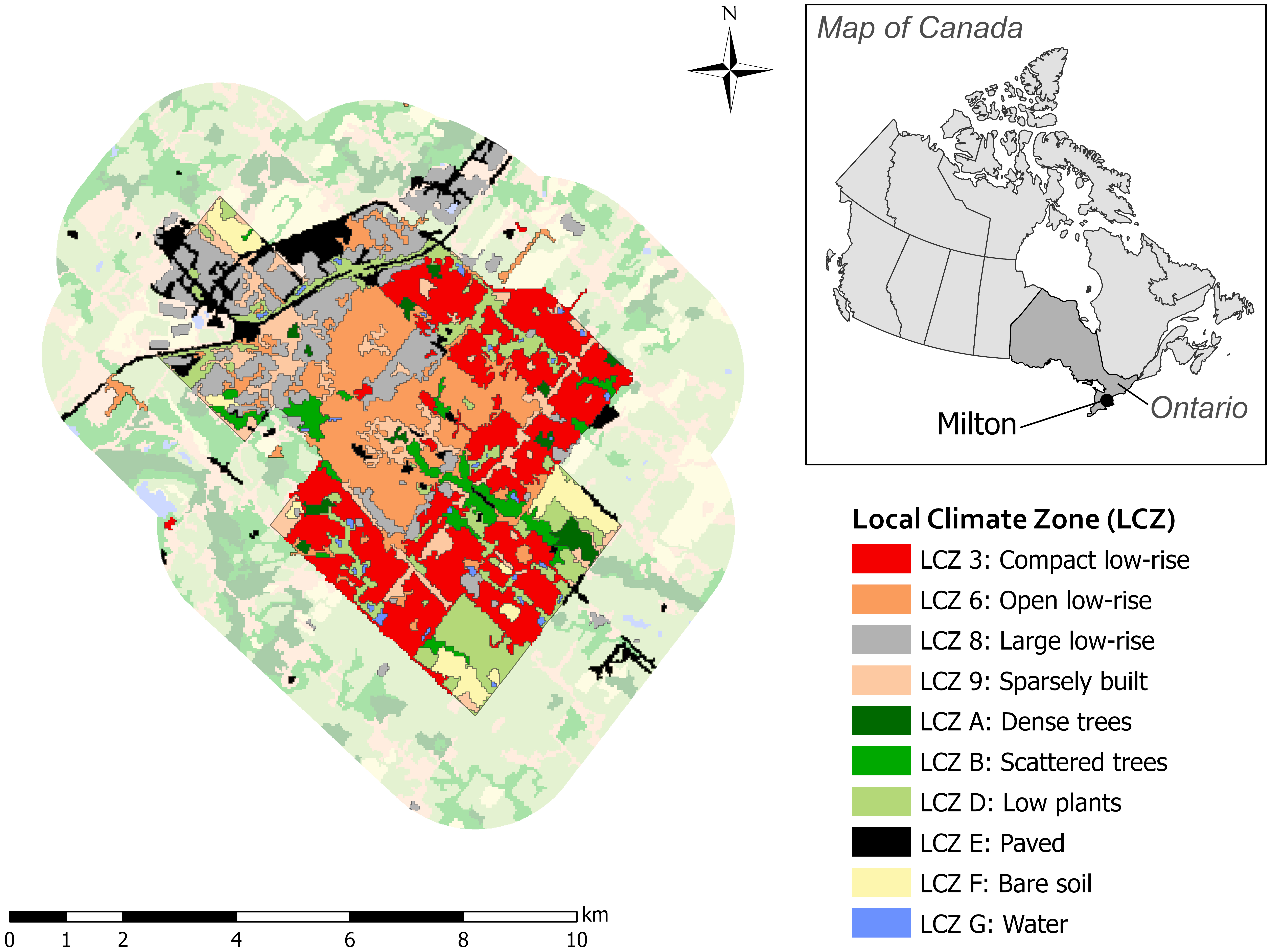
The RF object-based classification identified 10 homogeneous urban sub-classes based on the LCZs for Milton in 2019 at 30 m resolution (Fig. 1). All of the urban classes inside the socio-economic boundary of the buffered population centre were summed to give a total urbanized area for Milton. The total area calculated based on the RF object-based classification is 45.3 km2 (2019), while Statistics Canada’s official area for the population centre is 40.4 km2 (2016) (Table 9). The difference in area between the classification results and the official statistics (∼ 5 km2) is concentrated in the northeast area of the city and mainly represents paved areas (i.e., parking lots).
Table 9
Areas by local climate zone class
| LCZ | LCZ class | Area (km2) | % |
|---|---|---|---|
| 3 | Compact low-rise | 12.3 | 27.1 |
| 6 | Open low-rise | 8.3 | 18.2 |
| 8 | Large low-rise | 7.3 | 16.2 |
| 9 | Urban sparsely built | 3.9 | 8.7 |
| A | Urban dense trees | 0.8 | 1.7 |
| B | Urban scattered trees | 1.9 | 4.3 |
| D | Urban low plants | 5.0 | 11.1 |
| E | Paved | 3.6 | 7.9 |
| F | Urban bare soil | 1.8 | 2.7 |
| G | Urban water | 0.4 | 0.5 |
| Total urban | 45.3 | 100.0 |
Figure 1.
Milton urban local climate zones – 2019.
The application of the GEOBIA segmentation and classification approach delineated Landsat images segmented into spatially continuous and homogeneous regions according to LCZ classes based on spectral, spatial and contextual information. The error matrix calculated from the validation dataset demonstrated that the combination of Landsat8 spectral bands and NDVI with the Radarsat2 polarimetric decomposition parameters provided a more accurate urban characterization than the Landsat images alone (Table 5).
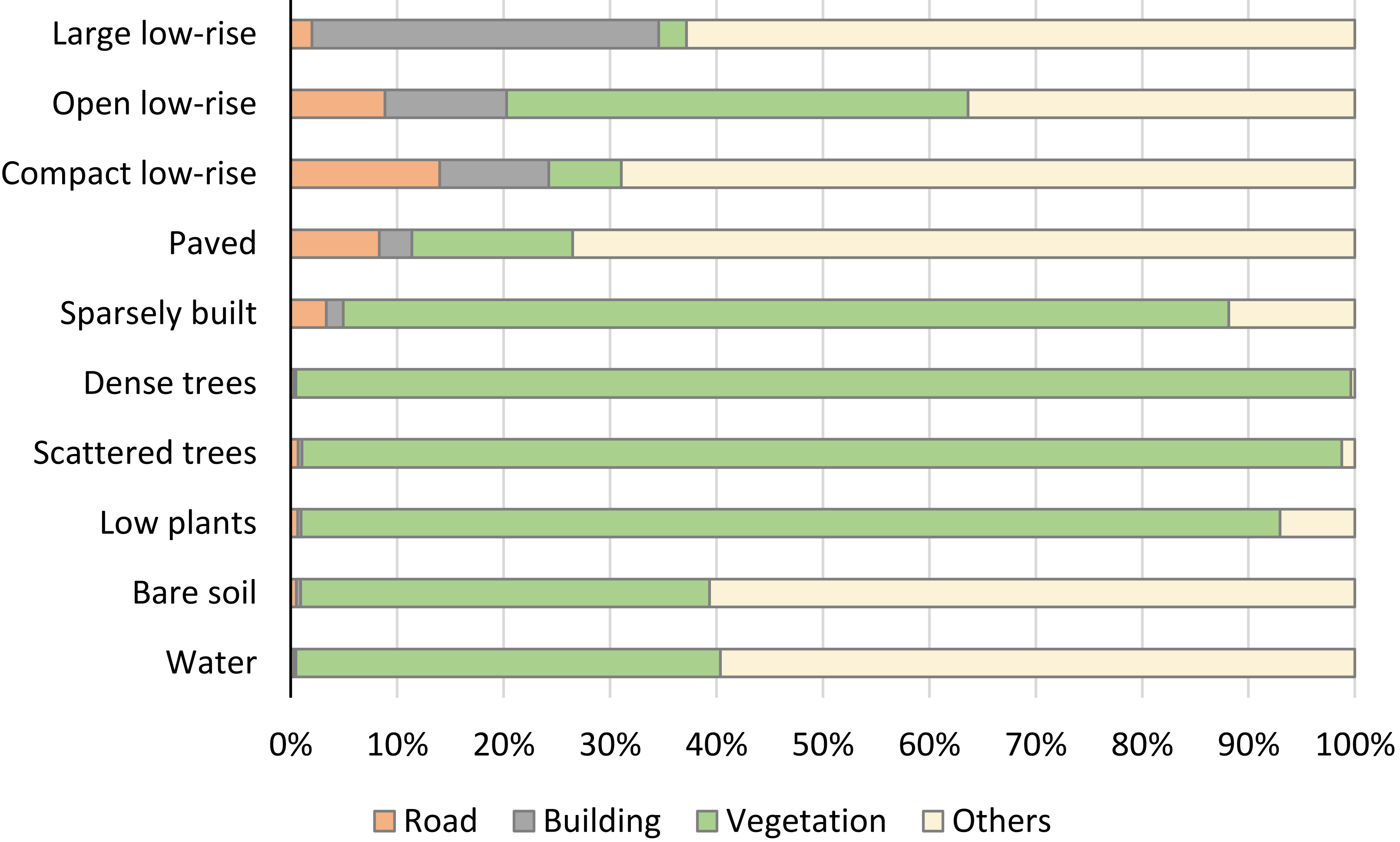
The use of ancillary geospatial datasets for measuring ecosystem assets can also be used to validate whether the pixel grouping produces meaningful results that meet urban ecosystem accounting requirements. The areas of buildings, buffered roads and vegetation were calculated for each LCZ class from the geospatial datasets described in the previous section. Limited information was available for impervious surfaces (e.g., parking lots), bare soil and water. These land cover classes were included as ‘Others’ by subtraction from the total area. Figure 2 provides the ratios of the building, road and vegetation areas for each LCZ class. The ratios are compliant with the description of the LCZ classes as described in Table 2 and as estimated by Stewart and Oke [13]. Note that the percentage of vegetation in the water class is caused by the inclusion of shorelines, islands and forest canopy in the object.
Figure 2.
Ratio of ecosystem assets by LCZ class.
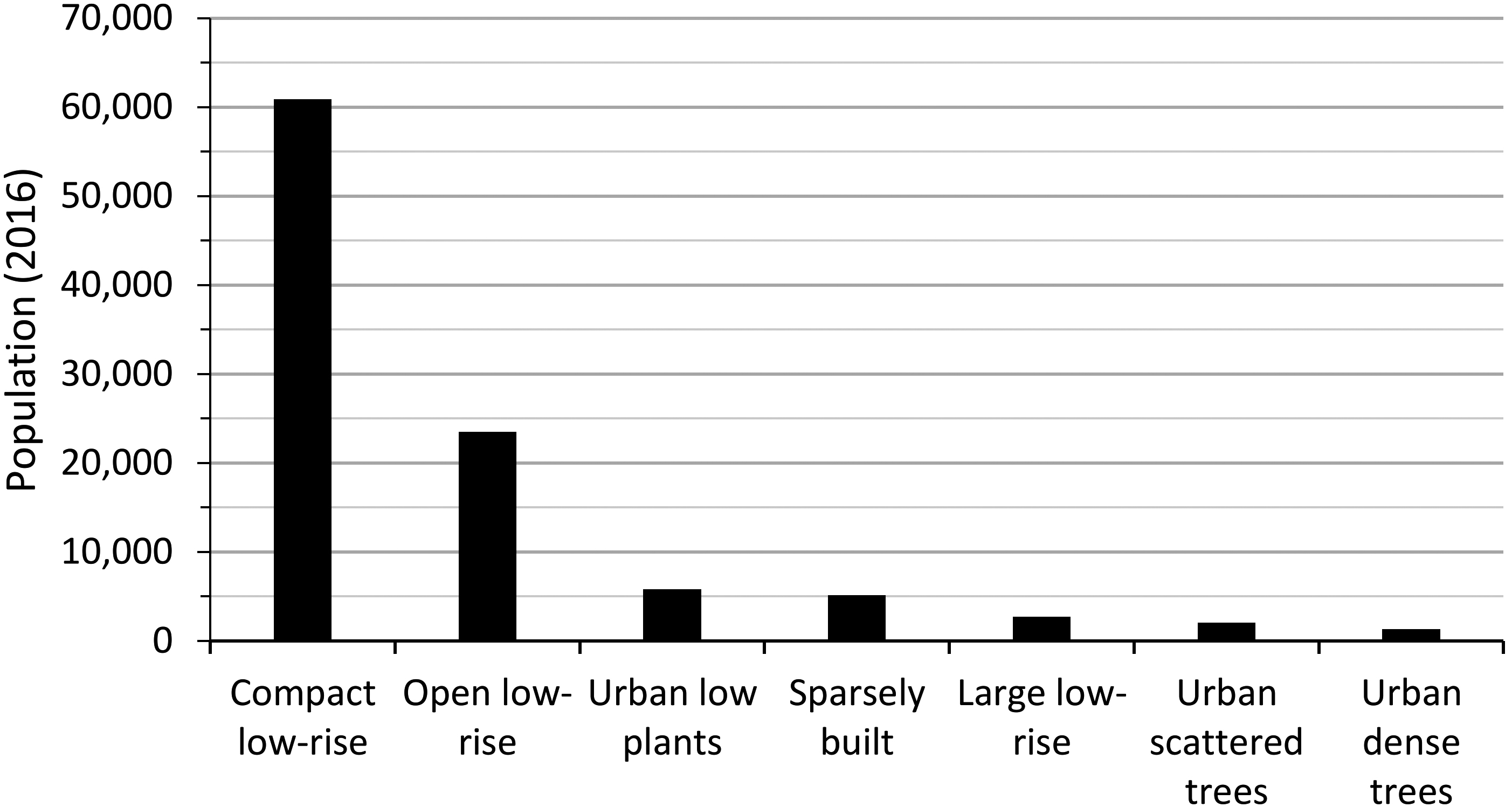
In defining the segments corresponding to the LCZ classes (or urban ecosystem types), it is helpful to consider how urban ecosystem assets differ in their ability to supply ecosystem services to people. For example, different levels of vegetation will impact climate regulation services in mitigating urban heat island effects. Figure 3 shows that the vegetated urban classes experienced lower temperatures compared to the urban classes where building and road area were more predominant, based on Landsat8 surface temperature data for August 1, 2019. The highest temperatures were seen in the Compact low-rise class, which also accounted for the largest proportion of the town’s population, indicating that a greater number of people were exposed to higher temperatures (Fig. 4).
Figure 3.
Surface temperature by LCZ for August 1, 2019.
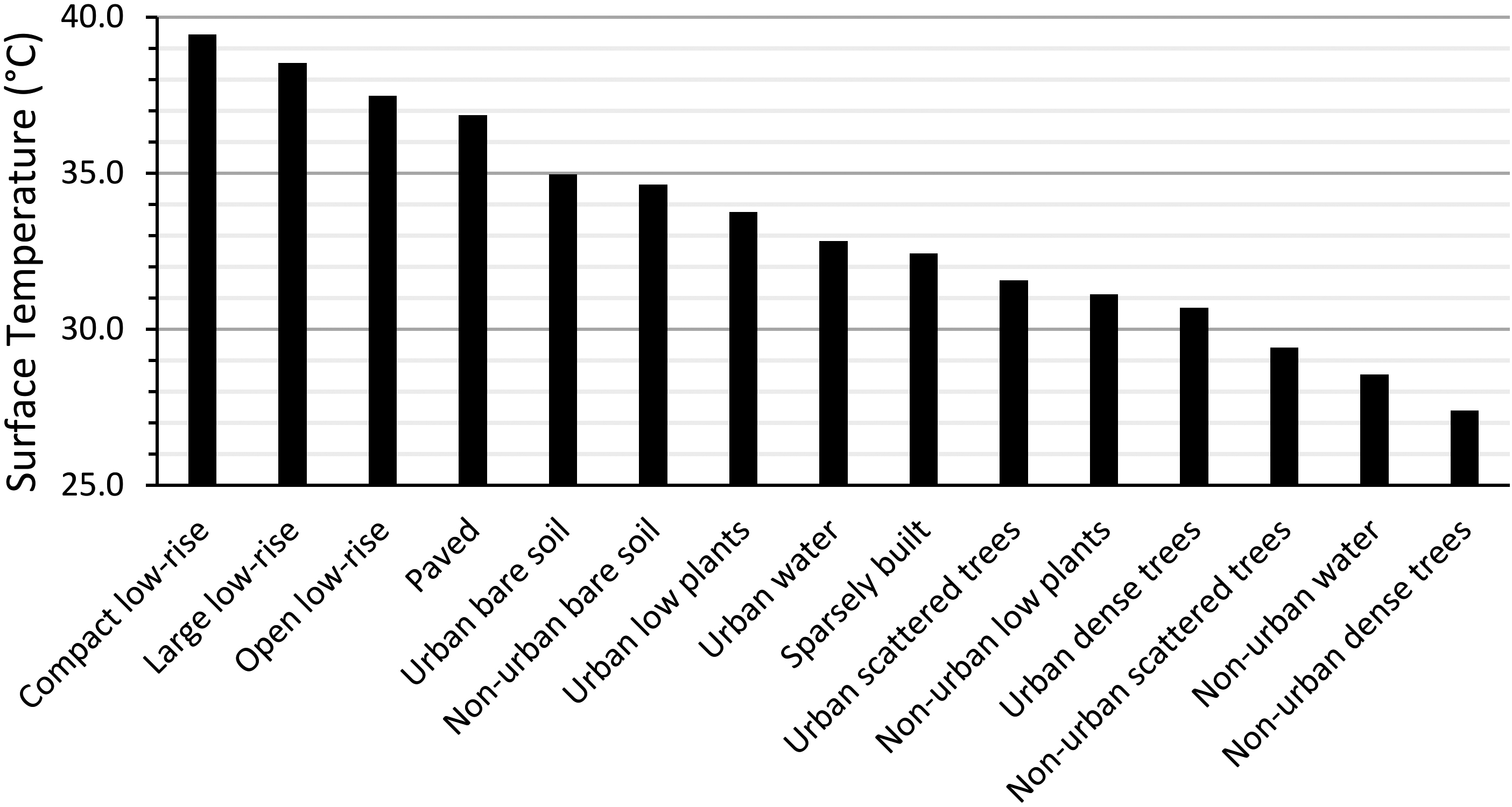
Figure 4.
Total population estimated by LCZ.
Changes in land cover composition are important landscape characteristics for assessing changes in ecosystem condition and functions. The object-based change detection analysis assessed the vegetation change at the landscape level (segment) using NDVI.
Figure 5 provides an example of the changes between 2001 and 2019 for one segment. The 2001 and 2006 sub-images show agriculture fields. Between 2006 and 2011, there was a conversion of agricultural fields to a combination of built-up and bare soil. Between 2011 and 2016, the entire object was converted to built-up area. Overall, 0.05 km2 of agricultural area was converted to built-up over the period. The analysis of NDVI for different years demonstrates that change in NDVI values can be used to identify both the type of change (i.e., conversion from agricultural to urban land uses) and when it occurs (Fig. 6).
Figure 5.
Changes observed in polygon 688 from Landsat series, 2001 to 2019.
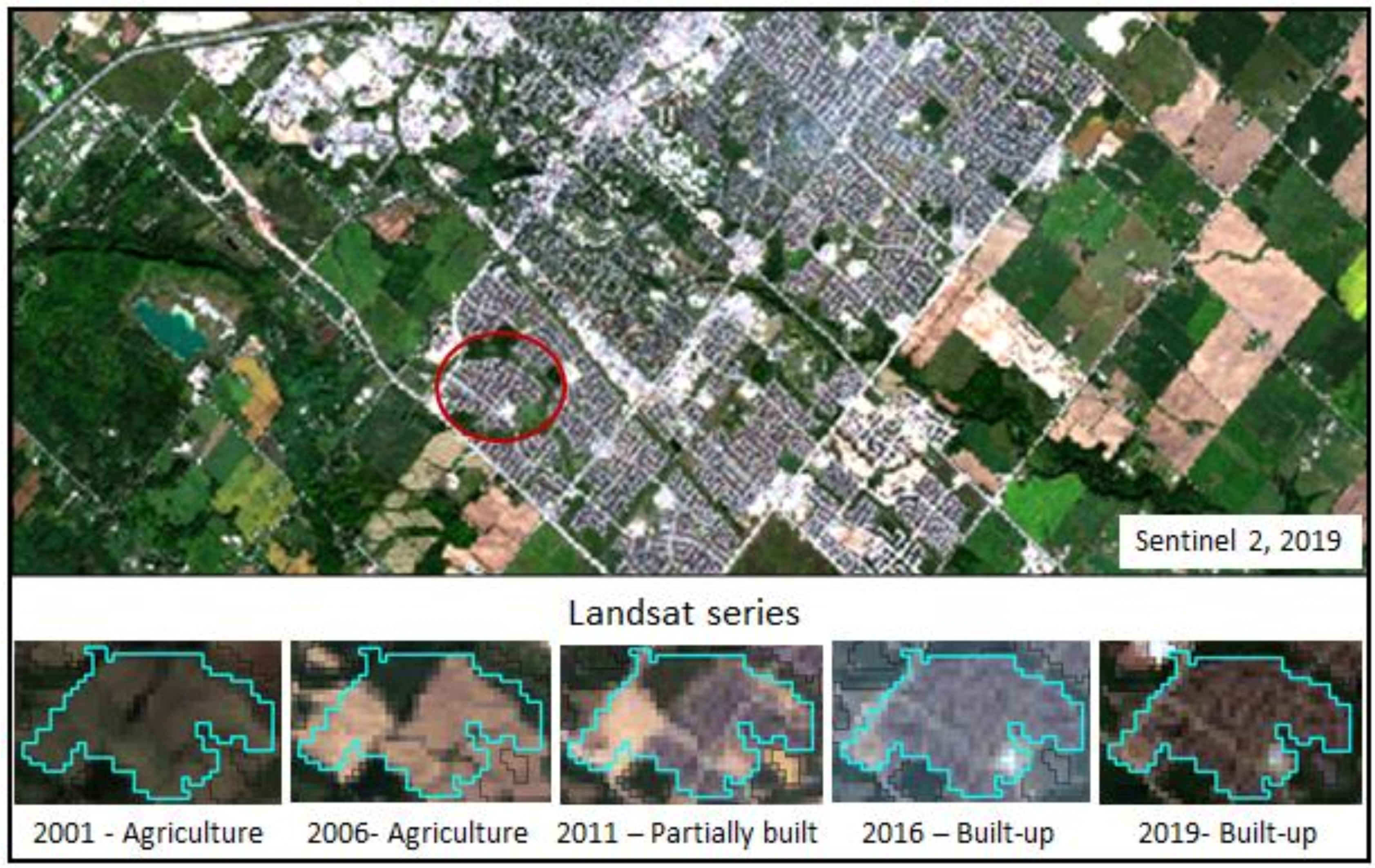
Figure 6.
Mean maximum NDVI values for polygon 688 from 2001 to 2019.
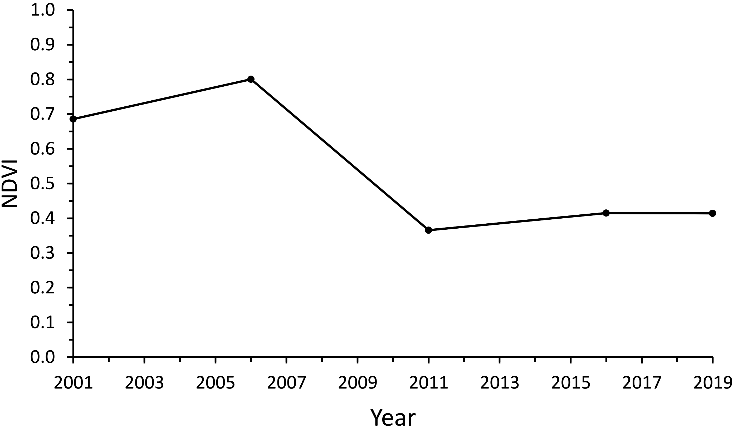
Figure 7.
Mean temperature for polygon 688 from 2001 to 2019.
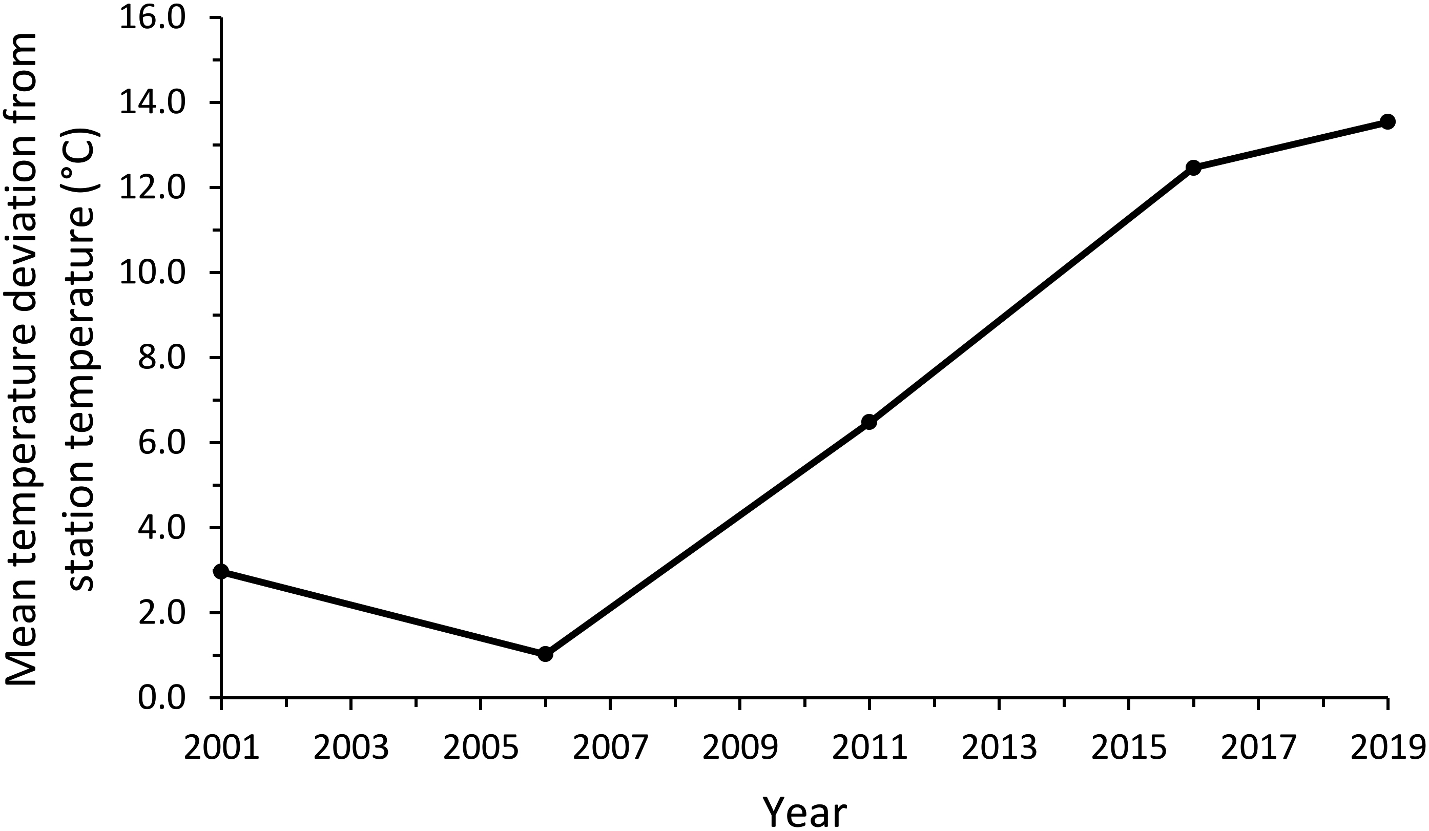
Changes in ecosystem characteristics have an impact on ecosystem conditions. For example, the surface temperature measured with Landsat8 (adjusted with ground sensors) demonstrated that the conversion of agricultural land (vegetated during the growing season) to built-up (buildings and impervious surface) correlates with an increased ground-level temperature (Fig. 7).
5.Conclusion and recommendations
This study investigated Radarsat-2 polarimetric parameters combined with Landsat data for urban delineation and characterization using object-based machine learning classifiers. The approach was successfully tested in Milton, Ontario, and is being applied at two other study sites in Drummondville, Quebec, and Richmond, British Columbia to evaluate its replicability before a broader application of the method to other population centres across the country. The goal would be to eventually apply this approach to the 1,005 population centres in Canada, which represent 28.6 million people or 81% of Canada’s total population, and approximately 18,000 km2 of urban area.
Based on the results, the following conclusions are drawn:
• Geographic object-based image analysis (GEOBIA) using the local climate zone (LCZ) classes provides a meaningful description of biophysical processes that can be used to define ecosystem services (e.g., temperature increase mitigation). Although developed for urban heat island studies, the LCZ classification provides representative groupings of individual urban components within urban ecosystems. The LCZ classification is flexible enough to apply to a wide variety of urban environments. An adoption of the approach used in this study could improve ecosystem accounts in other contexts and could be explored by other countries. The approach may work best in urban centres where urban planning and zoning results in developments with homogeneous urban types.
• The polarimetric parameters Alpha S, Lambda 1 and 3 (Touzi decomposition) and Maximum Intensity (Touzi discriminators) contributed to the improvement of the urban characterization following the LCZ scheme. The random forest classifier provided better results than the decision tree and support vector machine classifiers.
• The object-based change detection tracks the change at the patch (parcel) level, which is better adjusted to the heterogeneity of urban landscapes. The object-based approach combines the spectral properties of urban features reducing the effects associated with the single pixel that are not constant through time, thus the change detected at the object level represents a real conversion of land cover.
• Since the classifier is dependent on the quality and quantity of training and validation datasets, the selection of areas should be considered as a critical step toward the classification process. Sampling methodology should be scientifically and statistically sound. Moreover, a good coverage of the spatial variability of the training sites can contribute to the generation of unique set of spectral signature and/or polarimetric parameters, and then facilitate transferability between study sites.
Further research is needed to explore:
• Use of Sentinel-2 images with their resolution of 10 m, integrated with the Landsat images in the eCognition project, as this could improve the segmentation process, producing a more accurate and detailed delineation of the objects and facilitating the classification of the objects into LCZ classes.
• Use of cloud-based geospatial platforms, such as Google Earth Engine, to access imagery and enable analysis by facilitating scaling of the methodology to sites across the country.
• Assessment of the extent and condition of ecosystem assets through landscape metrics (e.g., fragmentation, connectivity, and mean patch size), which provide an accurate representation of the spatial arrangement by quantifying the extent and spatial characteristics at patch, classes or landscape level at different times.
The use of earth observation technologies to support official statistics remains a challenge, although methods based on earth observation for land use and land cover analysis are robust and scientifically recognized. Official statistics require that the data and documentation processes be compliant with the Quality Assurance Framework (QAF) [62] to ensure the credibility of the statistical agency. An assessment of products derived from remote sensing and earth observation data should consider the six dimensions of quality specified by the QAF including how they provide or support:
• Relevant information, through use of appropriate approaches (i.e., methodology, date and resolution), adapted to the purpose of the study.
• Accurate results, through documentation of errors and limitations.
• Improved timeliness of data, with the increased availability of satellite EO information (e.g., RADARSAT Constellation Mission (RCM) [63]).
• Accessible EO data that is openly available through portals and platforms (e.g., UN platform and Google Earth Engine), which also provide access to open source software and scripts, in addition to big data computing capacity for implementation at national and global scale.
• Improved coherence and comparability, through access to complete coverage of analysis ready data (ARD) ensuring the use of calibrated data at national scale.
• Interpretability provided by metadata standards.
The use of satellite earth observation approaches in accordance with these dimensions, will lead to lower costs and better services, contributing to the UN SEEA-EEA, assessments of climate change resilience, and other Statistics Canada programs related to urban areas.
Notes
Acknowledgments
This study was supported by Statistics Canada and the Canadian Space Agency. The authors would like to thank Dr. Ridha Touzi for advice on Radarsat polarimetric parameters; Katherine Strong for her support in mapping; Mark Henry for advice on ecosystem accounting and Dave Craig for his GIS analysis. The authors are grateful to the reviewers for their thoughtful comments which contributed to the improvement of this paper.
References
[1] | Ridd MK. Exploring a V-I-S (Vegetation-impervious surface-soil) model for urban ecosystem analysis through remote sensing: Comparative anatomy for cities. International Journal of Remote Sensing. (1995) ; 16: (12): 2165–2185. |
[2] | Lehner A, Blaschke T. A generic classification scheme for urban structure types. Remote Sensing. (2019) ; 11: (2): 173. |
[3] | United Nations. Technical Recommendations in support of the System of Environmental-Economic Accounting 2012 – Experimental Ecosystem Accounting. New York: United Nations; (2019) . Report No.: Series M No. 97. |
[4] | United Nations. Department of Economic and Social Affairs. [Online].; (2018) [cited 2019 March 20]. Available from: HYPERLINK https://www.un.org/development/desa/en/news/population/2018-revision-of-world-urbanization-prospects.html,%20. |
[5] | Wang J. Canada’s statistics on land cover and land use change in metropolitan areas. In 16th Conference of the International Association of Official Statisticians (IAOS) Urbanisation and sustainable cities. OECD Headquarters; (2018) ; Paris. |
[6] | AAFC. Agriculture and Agri-Food Canada, Annual Crop Inventory. [Online].; (2013) a [cited 2018 June 22]. Available from: HYPERLINK https://open.canada.ca/data/en/dataset/ba2645d5-4458-414d-b196-6303ac06c1c9. |
[7] | AAFC. Canada, Agriculture and Agri-Food, Land Use, 1990, 2000 and 2010; 2015. [Online].; (2018) [cited 2018 June 22]. Available from: HYPERLINK https://open.canada.ca/data/en/dataset/18e3ef1a-497c-40c6-8326-aac1a34a0dec. |
[8] | Latifovic R, Pouliot D, Olthof I. Circa 2010 land cover of canada: Local optimization methodology and product development. Remote Sensing. 1: (11): 1098. |
[9] | Elmqvist T, Setälä H, Handel SN, der Ploeg S, Aroson J, Blignaut JN, et al. Benefits of restoring ecosystem services in urban areas. Current Opinion in Environmental Sustainability. (2015) ; 14: : 101–108. |
[10] | FAO. Food and Agriculture Organization of the United Nations (FAO; Land Cover Classification System, Classification concepts. Software version 3. [Online].; (2016) [cited 2020 March 20]. Available from: HYPERLINK http://www.fao.org/3/a-i5232e.pdf. |
[11] | Jensen JR. Introductory Digital Image Processing: A Remote Sensing Perspective. 3rd ed. Upper Saddle River: Prentice Hall series in geographic information science; (2005) . |
[12] | Young CH, Jarvis PJ. Assessing the structural heterogeneity of urban areas: An example from the Black Country (UK). Urban Ecosystems. (2001) ; 5: : 49–59. |
[13] | Stewart ID, Oke TR. Conference notebook – A new classification system for urban climate sites. Bulletin of the American Meteorological Society. (2009) a; 90: : 922–923. |
[14] | USGS. United States Geological Survey, Landsat Data Access. [Online].; (2019) [cited 2019 June 20]. Available from: HYPERLINK https://www.usgs.gov/land-resources/nli/landsat/landsat-data-access?qt-science_support_page_related_con=0#qt-science_support_page_related_con. |
[15] | Zhang Y, Guindon B, Sun K. Concepts and application of the canadian urban land use survey. Canadian Journal of Remote Sensing. (2010) ; 36: (3): 224–235. |
[16] | Statistics Canada, Dictionary, Census of Population, 2016, Population centre (POPCTR). [Online].; (2016) [cited 2020 June 28]. Available from: HYPERLINK https://www12.statcan.gc.ca/census-recensement/2016/ref/dict/geo049a-eng.cfm. |
[17] | Statistics Canada, Population Ecumene Census Division Cartographic Boundary File, Reference Guide, 2016 Census. [Online].; (2016) [cited 2020 June 28]. Available from: HYPERLINK https://www150.statcan.gc.ca/n1/pub/92-159-g/92-159-g2016001-eng.htm. |
[18] | Pesaresi M, Ehrlich D, Ferri S, Florczyk AJ, Carneiro Freire SM, Halkia S, et al. Operating Procedure for the Production of the Global Human Settlement Layer from Landsat Data of the Epochs 1975, 1990, 2000, and 2014. European Commission, Joint Research Centre; (2016) a. Report No.: JRC No. JRC97705. |
[19] | Pesaresi MA, Florczyk AJ, Schiavina M, Melchiorri M, Maffenini L. European Commission, Joint Research Centre (JRC); GHS-SMOD R2019A – GHS settlement layers, updated ans refined REGIO model 2014 in application ot GHS-BUILT R2018A and GHS-POP R2019A, multitemporal (1975-1990-2000-2015). [Online].; (2019) [cited 2019 July 20]. Available from: HYPERLINK http://data.europa.eu/89h/42e8be89-54ff-464e-be7b-bf9e64da5218. |
[20] | Corbane C, Pesaresi M, Kemper T, Politis P, Florczyk AJ, Syrris V, et al. Automated global delineation of human settlements from 40 years of Landsat satellite data archives. Big Earth Data. (2019) ; 3: (2): 140–169. |
[21] | Feire S, MacManus K, Pesaresi M, Doxsey-Whitfield E, Mills J. Development of new open and free multi-temporal global population grids at 250 m resolution. In Geospatial Data in a Changing World; Association of Geographic Information Laboratories in Europe (AGILE). AGILE 2016; (2016) ; Helsinki. |
[22] | Florczyk AJ, Corbane C, Ehrlich D, Freire S, Kemper T, Maffenini L, et al. GHSL Data Package 2019. Data Package 2019. Luxembourg: European Union, Plubications Office; (2019) . |
[23] | Corbane C, Sabo F. European Settlement Map from Copernicus Very High Resolution data for reference year 2015, Public Release 2019. European Commission, Joint Research Centre (JRC). [Online].; (2019) [cited 2019 December 1]. Available from: HYPERLINK http://data.europa.eu/89h/8bd2b792-cc33-4c11-afd1-b8dd60b44f3b. |
[24] | Poursanidis E, Chrysoukakis K, Mitraka Z. Landsat 8 vs. Landsat 5: A comparison based on urban and peri-urban land cover mapping. International Journal of Applied Earth Observation and Geoinformation. (2015) ; 35: : 259–269. |
[25] | Salehi M, Sahebi MR, Maghsoudi Y. Improving the accuracy of urban land cover classification using Radarsat-2 PolSAR data. IEEE Journal of Selected Topics in Applied Earth Observations and Remote Sensing. (2014) ; 7: (4): 1394–1401. |
[26] | Corbane C, Politis P, Syrris V, Pesaresi M. GHS built-up grid, derived from Sentinel-1 (2016) R2018A. European Commission, Joint Research Centre (JRC). [Online].; (2018) [cited 2019 December 1]. Available from: HYPERLINK http://data.europa.eu/89h/jrc-ghsl-10008. |
[27] | Ban Y, Jacob A, Gamba P. Spaceborne SAR data for global urban mapping at 30 m resolution using a robust urban extractor. ISPRS Journal of Photogrammetry and Remote Sensing. (2015) May; 103: : 28–37. |
[28] | Höfer R, Banzhaf E, Ebert A. Delineating urban structure types (UST) in a heterogeneous urban agglomeration with VHR and TerraSAR-X data. In Joint Urban Remote Sensing Event; (2009) ; Shanghai. 1–7. |
[29] | Zhang H, Lin H, Whang Y. A new scheme for urban impervious surface classification from SAR images. ISPRS Journal of Photogrammetry and Remote Sensing. (2018) May; 139: : 103–118. |
[30] | Niu X, Ban Y. Multi-temporal RADARSAT-2 polarimetric SAR data for urban land-cover classification using an object-based support vector machine and a rule-based approach. International Journal of Remote Sensing. (2013) ; 34: (1): 1–26. |
[31] | Bhattacharya A, Touzi R. Polarimetric SAR urban classification using the Touzi target scattering decomposition. Canadian Journal of Remote Sensing. (2011) ; 37: (4): 323–332. |
[32] | Zhang H, Lin H, Li Y, Zhang Y, Fang C. Mapping urban impervious surface with dual-polarimetric SAR data: An improved method. Landscape and Urban Planning. (2016) July; 151: : 55–63. |
[33] | Esch T, Schenk A, Ullmann T, Thiel M, Roth A, Dech S. Characterization of land cover types in TerraSAR-X images by combined analysis of speckle statistics and intensity information. IEEE Transactions on Geoscience and Remote Sensing. (2011) ; 49: (6): 1911–1925. |
[34] | Esch T, Marconcini M, Felbier A, Roth A, Heldens W, Huber M, et al. Urban footprint processor; fully automated processing chain generating settlement masks from global data of the TanDEM-X mission. IEEE Geoscience on Remote Sensing, Letters. (2013) b; 10: (6): 1617–1621. |
[35] | Esch T, Heldens W, Hirner A, Keil M, Marconcini M, Roth A, et al. Breaking new ground in mapping human settlements from space – the global urban footprint. ISPRS Journal of Photogrammetry and Remote Sensing. (2017) December; 134: : 30–42. |
[36] | Esch T, Üreyen S, Metz-Marconcini A, Hirner A, Samer H, Tum M, et al. Exploiting big earth data from space – first experiences with the timescan processing chain. Big Earth Data. (2018) ; 2: (1): 36–55. |
[37] | Taubenböck H, Felbier A, Esch T, Roth A, Dech S. Pixel-based classification algorithm for mapping urban footprints from radar data: A case study for RADARSAT-2. Canadian Journal of Remote Sensing. (2012) ; 38: (3): 211–222. |
[38] | Ban Y, Hu H, Rangel IM. Fusion of quickbird MS and RADARSAT SAR data for urban land-cover mapping: Object-based and knowledge-based approach. International Journal of Remote Sensing. (2012) ; 31: (6): 1391–1410. |
[39] | Chen Z, Zhang Y, Guindon B, Esch T, Roth A, Shang J. Urban land use mapping using high resolution SAR data based on density analysis and contextual information. Canadian Journal of Remote Sensing. (2012) ; 38: (6): 738–749. |
[40] | Touzi R, Goze S, Le Toan T, Lopes A, Mougin E. Polarimetric discriminators for SAR images. IEEE Transactions on Geoscience and Remote Sensing. (1992) ; 30: (5): 973–980. |
[41] | Touzi R. Target scattering decomposition in terms of roll-invariant target parameters. IEEE Transactions on Geoscience and Remote Sensing. (2007) ; 45: (1): 73–84. |
[42] | Touzi R, Omari K, Sleep B, Jiao X. Scattered and received wave polarization optimization for enhanced peatland classification and fire damage assessment using polarimetric PALSAR. IEEE Journal of Selected Topics in Applied Earth Observations and Remote Sensing. (2018) November; 11: (1). |
[43] | Touzi R, Charbonneau F, Hawkins RK, Murnaghan K, Kavoun X. Ship-sea contrast optimization when using polarimetric SARs. In IGARSS 2001. Scanning the Present and Resolving the Future. Proceedings. IEEE 2001 International Geoscience and Remote Sensing Symposium (Cat. No. 01CH37217); 2001; Sydney. |
[44] | Benz U. Definiens Imaging GmbH: Object-Oriented Classification and Feature Detection. IEEE Geoscience and Remote Sensing Society Newsletter. (2001) ; 16–20. |
[45] | Momeni R, Aplin P, Boyd DS. Mapping complex urban land cover from spaceborne imagery: The influence of spatial resolution, spectral band set and classification approach. Remote Sensing. (2016) ; 8: (2). |
[46] | Qi L, Dou Y, Niu X, Xu J, Xu J, Xia F. Urban land use and land cover classification using remotely sensed SAR data through deep belief networks. Journal of Sensors, Special Issue: Deep Learning for Remote Sensing Image Understanding. (2015) ; 2015: : 10. |
[47] | Myint SO, Gober P, Brazel A, Grossman-Clarke S, Weng Q. Per-pixel vs. object-based classification of urban land cover extraction using high spatial resolution imagery. Remote Sensing of Environment. (2011) ; 115: (2011): 1145–1161. |
[48] | Pal M. Random forest classifier for remote sensing classification. International Journal of Remote Sensing, 26:1. (2005) ; 26: (1): 217–222. |
[49] | Üstüner M, Balik Sanli F, Abdikan S. Balanced vs Imbalanced Training Data: Classifying RapidEye Data with Support Vector Machines. In XXIII ISPRS Congress; (2016) ; Prague. 379–384. |
[50] | Sertel E, Akay SS. High resolution mapping of urban areas using SPOT-5 images and ancillary data. International Journal of Environment and Geoinformatics. (2015) ; 2: (2): 63–76. |
[51] | Nouri H, Beecham S, Anderson P, Nagler P. High spatial resolution WorldView-2 imagery for mapping NDVI and its relationship totemporal urban landscape evapotranspiration factors. Remote Sensing. (2014) ; 6: (1): 580–602. |
[52] | Chen G, Hay GJ, Carvalho LM, Wulder MA. Object-based change detection. International Journal of Remote Sensing. (2012) ; 33: (14): 4434–4457. |
[53] | Blaschke T. Toward a framework for change detection based on image objects. Göttinger Geogrphische Abbandlungen. (2005) January; 113: : 1–8. |
[54] | Ma L, Li M, Blaschke T, Ma X, Tiede D, Cheng L, et al. The effects of segmentation strategy, scale, and feature space on unsupervised methods. Remote Sensing. (2016) ; 8: (9): 761. |
[55] | Schneider A. Monitoring land cover change in urban and peri-urban areas using dense time stacks of Landsat satellite data and data mining approach. Remote Sensing of Environment. (2012) September; 124: : 689–704. |
[56] | Statistics Canada, Census Profile, 2016 Census. [Online].; (2017) [cited 2019 January 15]. Available from: HYPERLINK https://www12.statcan.gc.ca/census-recensement/2016/dp-pd/prof/index.cfm?Lang=E%20. |
[57] | PCI Geomatics, SAR Processing with Geomatica, Geomatica Training Guide V 2.4. [Online].; (2016) [cited 2019 June 20]. Available from: HYPERLINK https://www.pcigeomatics.com/pdf/training-guides/2016/SAR.pdf. |
[58] | Statistics Canada, Dictionary, Census of Population, 2016, Population centre (POPCTR). [Online].; (2016) [cited 2019 June 20]. Available from: HYPERLINK https://www150.statcan.gc.ca/n1/en/catalogue/92-166-X. |
[59] | Statistics Canada, Road Network File. [Online].; (2016) [cited 2020 January 20]. Available from: HYPERLINK https://www150.statcan.gc.ca/n1/en/catalogue/92-500-X. |
[60] | Microsoft, Canadian Building Footprints. [Online].; (2019) [cited 2019 November 1]. Available from: HYPERLINK https://github.com/microsoft/CanadianBuildingFootprints/commit/0d2f8f5796ea2d2a7a5bcfa079c635ba3f2e8bc0. |
[61] | Olofsson P, Foody GM, Herold M, Stehman SV, Woodcock CE, Wulder MA. Good practices for estimating area and assessing accuracy of land change. Remote Sensing of Environment. (2014) ; (148): 42–57. |
[62] | Statistics Canada, Quality Assurance Frameworks. [Online].; (2017) [cited 2019 June 20]. Available from: HYPERLINK https://www150.statcan.gc.ca/n1/en/pub/12-586-x/12-586-x2017001-eng.pdf?st=GvcAaB5H. |
[63] | Canadian Space Agency, Radarsat Constellation Mission (RCM). [Online].; (2019) [cited 2019 December 1]. Available from: HYPERLINK https://www.asc-csa.gc.ca/eng/satellites/radarsat/default.asp. |

