
qEndpoint: A novel triple store architecture for large RDF graphs
Abstract
In the relational database realm, there has been a shift towards novel hybrid database architectures combining the properties of transaction processing (OLTP) and analytical processing (OLAP). OLTP workloads are made up by read and write operations on a small number of rows and are typically addressed by indexes such as B+trees. On the other side, OLAP workloads consists of big read operations that scan larger parts of the dataset. To address both workloads some databases introduced an architecture using a buffer or delta partition.
Precisely, changes are accumulated in a write-optimized delta partition while the rest of the data is compressed in the read-optimized main partition. Periodically, the delta storage is merged in the main partition. In this paper we investigate for the first time how this architecture can be implemented and behaves for RDF graphs. We describe in detail the indexing-structures one can use for each partition, the merge process as well as the transactional management.
We study the performances of our triple store, which we call qEndpoint, over two popular benchmarks, the Berlin SPARQL Benchmark (BSBM) and the recent Wikidata Benchmark (WDBench). We are also studying how it compares against other public Wikidata endpoints. This allows us to study the behavior of the triple store for different workloads, as well as the scalability over large RDF graphs. The results show that, compared to the baselines, our triple store allows for improved indexing times, better response time for some queries, higher insert and delete rates, and low disk and memory footprints, making it ideal to store and serve large Knowledge Graphs.
1.Introduction
Hybrid transactional and analytical processing (HTAP) is a term coined in the relational database world, to indicate database system architectures performing real-time analytics combining read and write operations on a few rows with reads and writes on large snapshots of the data [15]. Combining transactional and analytical query workloads is a problem that has not been yet tackled for RDF graph data, despite its importance in future Big graph ecosystems [24]. Inspired by the relational database literature, we propose a triple store architecture using a buffer to store the updates [11,25]. The key idea of the buffer is that most of the data is stored in a read-optimized main partition and updates are accumulated into a write-optimized buffer partition we call delta. The delta partition grows over time due to insert operations. To avoid the situation that the delta partition becomes too large thus leading to deteriorated performances, the delta partition is merged into the main partition. One would expect the following advantages of such an architecture:
 higher read performance, due to the read-optimized main partition
 faster insert performance, since only the write-optimized partition is affected;
 faster delete performance, since the write-optimized partition is smaller and deletions in the main partition are just marking data as deleted;
 smaller indexing size and smaller memory footprint, since the main partition is read only and therefore higher compression on the data can be applied
 faster indexing speed, since all initial data does not need to be stored in a data structure that is updated over time while more an more data is indexed.
 better performance on analytical queries. since the read-optimized partition allows for faster scans over the data
This paper is organized as follows. In Section 2, we describe the related works. In Section 3, we describe the data-structures that we use for the main-partition and for the delta-partition. In Section 4, we describe how SELECT, INSERT and DELETE operations are carried out on top of the two partitions. In Section 5, we describe the merge operation. In Section 6, we carry out a series of experiments that compare the performance of this new architecture with existing ones. A Supplemental Material Statement in Section 8. We conclude with Section 9 where we discuss the advantages and limitations of our proposed architecture.
2.Related work
Relational database systems are the most mature systems combining transaction processing (OLTP) and analytical processing (OLAP) [11,18]. OLTP workloads are made up by read-and write operations on a small number of rows and are typically addressed by B+Trees. On the other side OLAP are made up by big read and write transactions that scan larger parts of the data. These are typically addressed using a compressed column-oriented approach [1]. To address both workloads, the differential update architecture has been introduced [11] combining a write-optimized delta partition and a read-optimized main partition. This process is called merge [17,18]. One of the main advantages of the main partition is not only that it is read-optimized, but also that it is compressed allowing to load in memory much bigger parts of the data.
Many different architectures have been explored for graph databases. We limit ourselves to describe the common options and we refer to [2] for a more extensive survey. A very common architecture for triple stores is based on B+-trees. These are used for example in RDF-3X [21], RDF4J [8] Blazegraph and Apache Jena. These allow for fast search as well as delete and insert operations.
Another line of work tries to map the graph database model on an existing data model. For example, Trinity RDF [29] maps the graph data model to a key value store. Another approach is to use the relational database model. This is done for example in Virtuoso [9] or SAP HANA Graph [16] where all RDF triples are stored in a table with three columns (subject, predicate, object). Also, Wilkinson et al. [28] uses the relational database model but in this case a table is created for each property in the dataset.
There are two lines of work that are most similar to ours. The first are works that use read-only compressed data structures rather than B+-trees to store the graph like QLever [4]. However, they do not support updates and are only limited to the main partition. The second are versioning systems where the data is stored in a main partition and changes are stored in a delta partition. This is the case of x-RDF-3X [22] relaying on RDF-3X and OSTRICH [26] relaying on HDT. OSTRICH, unlike our system, gives access to the data only via triple pattern searches with the possibility to specify a start or end version. Their aim is not to have an efficient SPARQL endpoint. x-RDF-3X on the other side, is built on top of RDF-3X which, as mentioned above, is a B+-trees and not on compressed data structure. Moreover this system isn’t maintained anymore.
3.Data structures for main and delta-partition
In order to construct a differential update architecture we need to choose data-structures that are well suited for the main-partition and the delta-partition, we respectively HDT and the RDF4J native store. We describe our choices for qEndpoint.
3.1.RDF
In qEndpoint, we are using RDF graphs. RDF is a widely used data model in the Semantic Web. It relies on the notions of RDF triples and RDF triple patterns.
RDF triple and RDF triple pattern Given an infinite set of terms
– An RDF triple is a tuple
– An RDF triple pattern is a tuple
RDF graph An RDF graph
RDF triple pattern resolution function Let
– We say that an RDF triple
∗ if
∗ if
∗ and if
– We call a function:
3.2.HDT: The main partition
The main partition should be a data-structure that allows for fast triple-pattern retrieval and has high data compression. For this we choose HDT [12]. HDT is a binary serialization format for RDF based on compact data structures. These aim to compress data close to the possible theoretic lower bound, while still enabling efficient query operations. More concretely HDT has been shown to compress the data to an order of magnitude similar to the gzipped size of the corresponding n-triple serialization, while having a triple pattern resolution speed that is competitive with existing triples-stores. This makes it an ideal data structure for the main-partition.
In the following we are describing the internals of HDT that are needed to understand the following of the paper. HDT consists of three main components, namely: the header (H), the dictionary (D) and the triple (T) partition.
The header component is not relevant, as it stores metadata about the dataset like number of triples, number of distinct subjects and so on.
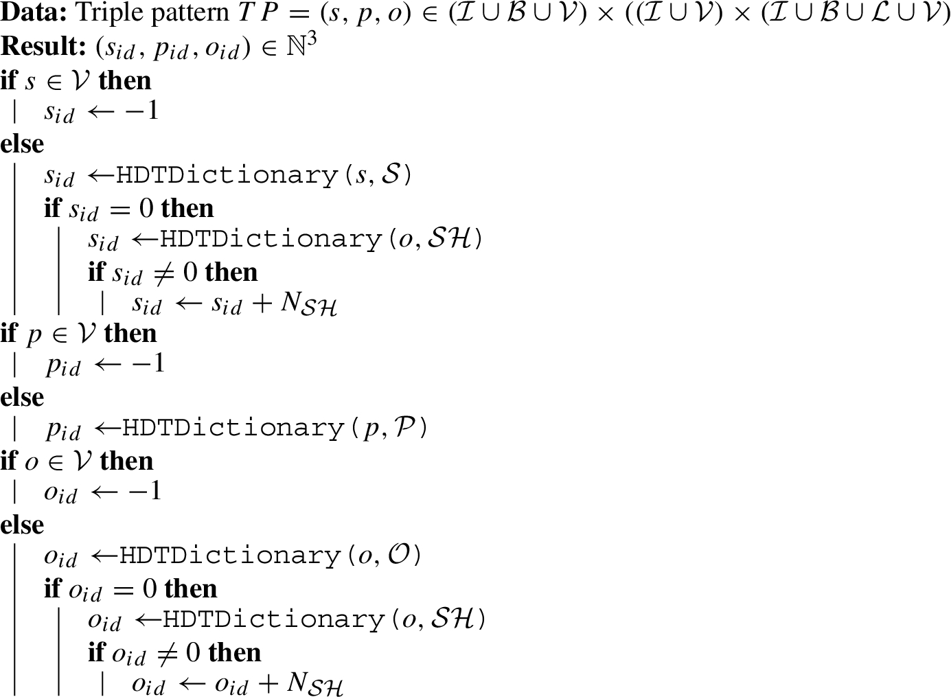
The dictionary is a map that assigns to each IRI, blank node, and literal (which we will call resources in the follow) a numeric ID. The dictionary is made up by 4 sections (
The ID is 0 if the term does not exist in the corresponding section.
The triples are encoded using the IDs in the dictionary and then lexicographically ordered with respect to subject, predicate and object. These are encoded using two numeric compact arrays and two bitmaps. This data structure allows for fast triple pattern resolution for fixed subject or fixed subject and predicate. With HDT FoQ [20], an additional index data structure is added to query the triple patterns
Most importantly, HDT offers APIs to search for a given triple pattern either by using resources or by using IDs. It returns triples together with their
Last but not least, we would like to point out that an HDT file can be queried either in “load” or “map” mode. In the “load mode”, the entire data set is loaded into memory. In the “map mode”, the HDT file is “mapped” in the endpoint memory, only parts of the file are loaded into memory when required.
3.3.RDF-4J native store: The delta-partition
The delta-partition should be a write-optimized data structure. B+-trees offer a good trade-off between read speed while maintaining good write performance. Moreover B+-trees are widely used in many triple-stores showing that they are a good choice for triple-stores in general. Finally B+-trees are also used as the delta-partition in the relational database world. We therefore choose for the delta-partition the RDF4J native store which is an open source, maintained and well optimized triple-store back-end that relies on B+-trees.
Due to space reasons, we do not provide details about the internals of RDF4J since they are not important to understand the following. Despite HDT, an RDF4J store
4.Select, insert and delete operations
In qEndpoint, we are using the RDF4J SPARQL 1.1 API, giving us access to a premade SPARQL implementation. To connect the API to our store we need to indicate how to SELECT, INSERT and DELETE one RDF triple pattern. All other SPARQL operations are build on top of these elementary operations. For now the transaction aren’t supported above the NONE level.33
It is important to make the destinction between the RDF4J Native Store and the RDF4J SPARQL API. These are two projects of the RDF4J library, but are independent components of qEndpoint. The NativeStore is used in the storage and the SPARQL API to provide an interface between the endpoint and the storage.
Fig. 1.
The main components of qEndpoint.
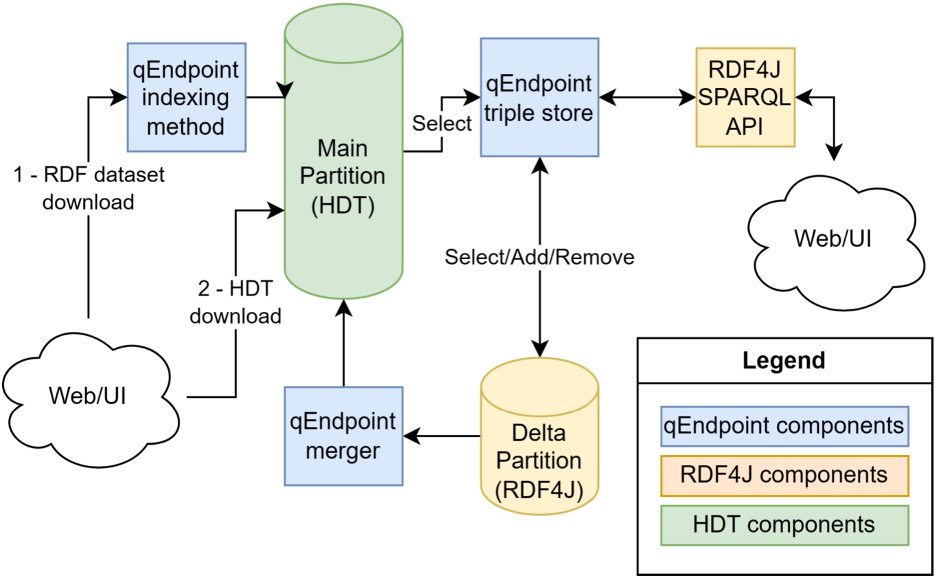
The qEndpoint system architecture is inspired by that of the relational database SAP HANA [18], one of the first commercial database to propose updates with a buffer architecture. This paper is inspired by the SAP HANA’s merge process, i.e. which data structures are used, how transactions are locked, how the data is moved from the main to the delta partition [17]. In a nutshell, the data is stored in a compressed read-optimized main partition and a write-optimized delta partition kept alonside (see Fig. 1). The main partition is handled via HDT, which is highly compressing RDF datasets and can reach 10x compression factors. Moreover, the data structures of HDT are read-optimized for fast triple-pattern resolution and can compete in this respect with traditional triple stores. The delta partition is handled with the RDF4J native store, which is known to have good performances especially for dataset sizes of up to 100M triples.44 The system can be accessed using either the user interface (UI) or via the web API. When a dataset is uploaded to the endpoint, we are using a custom indexing method to index the dataset into the main partition with a low-memory footprint. Once the delta partition becomes too big, a merge process (qEndpoint merger in the figure) is triggered to add the triples from the delta partition to the main partition.
Algorithm 1:
HDTTriplesID retrieve HDT id from triple pattern
– SELECT: both the HDT main partition and the RDF4J delta partition offer triple pattern resolution functions, we denote them as HDTTriples(
∗ Using the strategy above, we would, for each triple pattern resolution, make calls to the HDT dictionary and convert a triple ID back to a triple pattern. This is very costly and in many cases not necessary. When joining multiple triples we do not need to know the triples themselves, but only if the subject, predicate, object are equal (and the ID suffice for this operation). Whenever possible, we therefore avoid the tripleID conversions. On the other hand, for example for FILTER operations we need the value of some of the resources in the triple and in these cases we convert the IDs to their corresponding string representations. This is also done when the actual result is returned to the user.
In order to make all joins over IDs, the triples stored in the delta-partition need to be stored via IDs (otherwise a conversion of the IDs via the dictionary is unavoidable). We therefore store every resource in the delta-partition with its HDT ID (if it exists) using the particular IRI format http://hdt.org/{section}{id}, where section is S/SH/P/O for each HDT section and id the HDT ID.
Finally note that, as described above in Section 3.2, a predicate and a subject/object can have the same ID but represent different resources. This means that if a subject or object ID is used to query in predicate position (or the other way around) then the conversion over the dictionary is unavoidable.
∗ When searching over IDs, some HDT internals are exploited to cut down certain search operations. For example, from an object ID, one can check whether it also appears as a subject. Triple patterns that in the subject position have IDs of objects that by their ID range cannot appear as object, also do not need to be resolved.
∗ Using the above strategy, we would, for each triple pattern, search over HDT and also search over RDF4J. In general, we assume that most of the data is contained in HDT and most of these calls will return empty results. On the other hand, these calls are expensive. To avoid them we add a new data structure in qEndpoint. For each entry in the HDT dictionary, we add a bit that indicates if the corresponding entry is used in the RDF4J store (as explained later in the INSERT part). We call it XYZBits. If a triple pattern contains resources contained in HDT, we check the XYZBits. We search the triple pattern over the RDF4J store if and only if the bit for all the resources in the triple pattern are set.
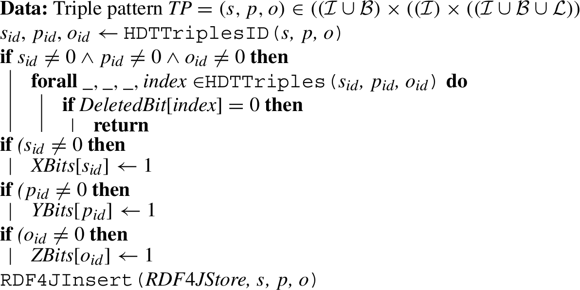
– INSERT: the insert operation is affecting only the RDF4J delta. When a triple is inserted, we check against the HDT dictionary if the subject, predicate, object are present in the HDT dictionary. If this is the case we store the corresponding resource using the HDT IDs in RDF4J. Moreover, in this case, we mark the corresponding bits in the XYZBits data structure. Note that the RDF4J store contains a mixture of “plain” resources and IDs (see Algorithm 2).
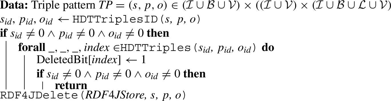
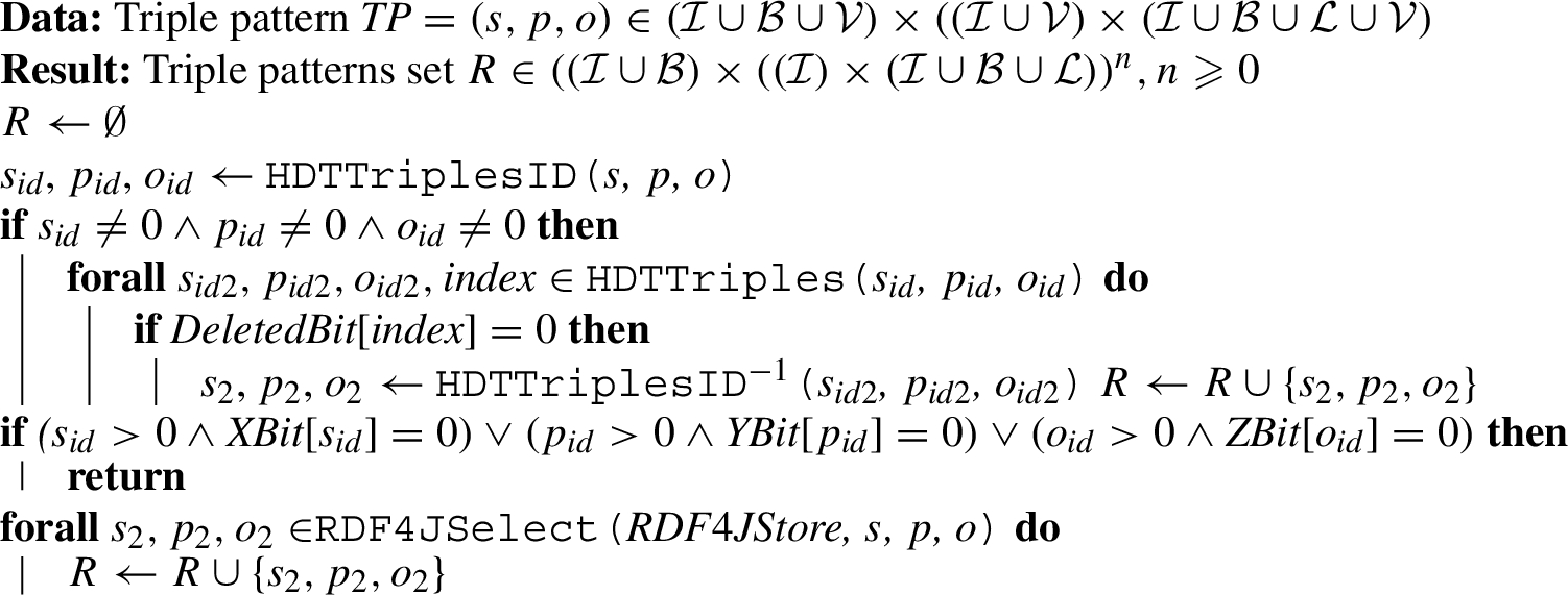
– DELETE: when a triple is deleted, we need to delete it in the main partition and in the delta, depending where it is located. Deleting a triple in the delta is not a problem since this functionality is directly provided. HDT on the other side does not have the concept of deletion. In HDT, each triple is naturally mapped to an ID and the triples are lexicographically ordered. We exploit this by adding a new data structure conceived to handle deletions. It consists of a bit sequence of the length of the number of triples in HDT. We call it “DeletedBit”. We use it to mark a triple as deleted. This is achieved by searching the triple over HDT, computing its position and marking the corresponding bit. Note that HDT does not provide APIs to retrieve, given a triple, its corresponding ID. We have therefore implemented this functionality in qEndpoint (see Algorithm 3). This part is also reflected in the SELECT algorithm, when a triple is queried, the DeletedBit sequence is checked to avoid this triple (see Algorithm 4).
Algorithm 2:
Insert a triple into the RDF graph
Algorithm 3:
Delete a triple from the RDF graph
Algorithm 4:
Select a triple of the RDF graph
Notice that the above operations allow to achieve a SPARQL 1.1-compliant SPARQL endpoint, given that the SPARQL algebra is build upon these operations. We carry out two further optimizations, as follows. First, we reuse the query plan generated by RDF4J. In particular, this means that all join operations are carried out as nested joins. Second, we need to provide the query planner with an estimate of the cardinality for the different triple patterns. These are used to compute the correct query plan. We compute the cardinality by summing the cardinality given by HDT with the one given by RDF4J. While the cardinalities provided by RDF4J are estimations, the cardinalities provided by HDT are exact. This allows the generation of more accurate query plans.
Our system was built on top of the RDF4J API to provide a SPARQL endpoint, allowing the delta partition to be replaced with any triple store integrated using the RDF4J Sail API.55 Unlike with the delta partition, with the main partition the optimizations explained in section doesn’t allow a trivial replacement to another main partition.
5.Merge
As the database is used, more data accumulates in the delta. This is problematic since the delta store cannot scale. We therefore trigger merges in which the data in the delta is moved to the HDT main partition so that the initial state of an empty delta is restored.
There are two problematic aspects there. The first is how to move the data from the delta-partition to the main partition in an efficient way. The second is how to handle the transactions.
5.1.HDTCat and HDTDiff
To move the data from the delta-partition to the main partition the naive idea would be to dump all data from the delta-partition uncompress the HDT main partition, merge the data and compress it back. This approach is not efficient, neither in terms of time nor in terms of memory footprint. We therefore rely on HDTCat [6], a tool that was created to join two HDT files without the need of uncompressing the data. The main idea of HDTCat is based on the following observation. HDT is a sorted list of resources (i.e. the dictionary containing URIs, Literals and blank-nodes) as well as a sorted list of triples. This is true up to, the splitting of the dictionary in different sections, and the compression of the sorted lists. This means that merging to HDTs corresponds to merge two ordered lists which is efficient both in time and in memory.
On the other side in the merge operation we do not need only to add data, but also to remove the triples that are marked as deleted. We therefore developed HDTDiff, a method to remove from an HDT file triples marked as deleted using the main partition delete bitmap.
HDTDiff will first create a bitmap for each section of the HDT dictionary (Subject, Predicate and Object) and fill them using the delete bitmap. If a bit is set to one at the index i of a bitmap for the section S, it means the element i of the section s is required by the future HDT. At the end of the bitmap building, with the result HDT, we use a similar method, HDTCat to compute the final HDT without the triples.
Note that HDTCat and HDTDiff do not assume that the underlying HDTs are loaded in memory, the HDT file and the bitmaps are only mapped from disk. By reading the HDT components sequentially without any random memory access, these operations are not memory intense and hence scalable.
After this step, the delta partition is now empty and the main partition is containing all the triples of dataset. Allowing us to fill again the delta partition while having our previous data compressed with the main partition.
5.2.Transaction handling
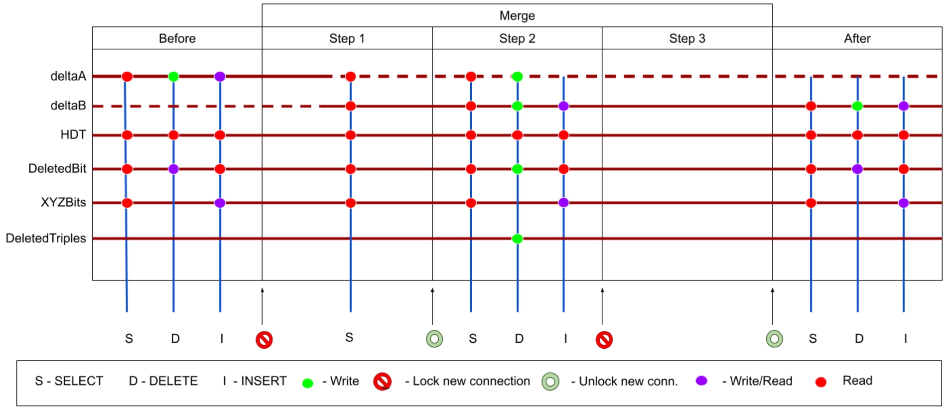
In the following, we detail the merge operation (see Fig. 2), that takes place in 3 steps.
Fig. 2.
Figure detailing the merge operation. Horizontally we depict the different merge steps. In each step we detail which operations (SELECT (S), DELETE (D) and INSERT (I)) is possible. Moreover, we vertically depict the data structures that are accessed by the corresponding operation.
5.2.1.Step 1
This step is triggered by the fact that the delta has exceeded a certain number of triples (which we call threshold). Step 1 locks all new incoming update connections. Once all existing update connections terminate, a new delta is initialized, which will co-exist with the first one during the merge process. We call them deltaA and deltaB, respectively, and they ensure that the endpoint is always available during the merge process. Also, a copy of DeletedBit is made called DeletedBit_tmp. The lock on the updates ensures that the data in the delta and in DeletedBit is not changed during this process. Once the new store is initialized, the lock on update connections is released.
5.2.2.Step 2
In this step, all changes in the delta are moved into the main partition. In particular, the deleted triples in (DeletedBit_tmp) and the triples in the deltaA storage are merged into the main partition. This is carried out into two steps using hdtDiff and hdtCat. The use of hdtCat and hdtDiff is essential to maintain the process scalable since decompressing and compressing an HDT file is resource intense (in particular with respect to memory consumption). When the hdtDiff and hdtCat operations are finished, a new HDT is generated that needs to be replaced with the existing one and step 3 is triggered. In step 2, SELECT, INSERT and DELETE operations are allowed. SELECT operations need access to the HDT file as well as the deltaA and deltaB store. INSERT operations will only affect deltaB, while DELETE operations will affect the delete bitmap bits, deltaA and deltaB. Moreover, all deleted triples will also be stored in a file called DeletedTriples.
5.2.3.Step 3
This step is triggered when the new HDT is generated. At the beginning, we lock all incoming connections, both read and write. At the beginning of this step, the XYZBits are initialized using the data contained in deltaB. Furthermore, a new DeletedBit is initialized. To achieve this, we iterate over the triples stored in DeletedTriples and mark these as deleted.
Moreover, the IDs used in deltaB are referring to the current HDT. We therefore iterate over all triples in deltaB and replace them with the IDs in the new HDT. During this process there is a mixture of IDs used in the old and the new HDT, which explains why we also lock read operations. We finally switch the current HDT with the new HDT and we release all locks restoring the initial state.
6.Experiments
In this section we show two evaluation results of the qEndpoint. In the first we evaluate qEndpoint over the Berlin SPARQL benchmark [5],66 a synthetic benchmark that allows to test a SPARQL endpoint under different query loads in read (select), read-write (update) and analytic (business intelligence) scenarios. In the second we evaluate WDBench [3], a SPARQL benchmark based on the Wikidata query logs. You can find the git repository with the experiments at [23]. It gives us a synthetic and a real world data benchmark to have the two references in our results.
Table 1
Loading times and result index size for different dataset sizes and stores
| Product count | Triple count | NTriple size | qEndpoint index | RDF4J index | ||
| Loading | Size | Loading | Size | |||
| 10 k | 3,53M | 871 MB | 38 s | 191 MB | 1 m 38 s | 476 MB |
| 50 k | 17,5M | 4.3 GB | 3 m 17 s | 933 MB | 10 m 8 s | 2.3 GB |
| 100 k | 34,9M | 8.5 GB | 6 m 47 s | 1.9 GB | 26 m | 4.6 GB |
| 200 k | 69,5M | 18.2 GB | 13 m 17 s | 3.6 GB | 55 m | 9 GB |
| 500 k | 174M | 45.6 GB | 35 m | 9 GB | 3 h 25 m | 23 GB |
| 1 M | 347M | 86 GB | 1 h 23 m | 18 GB | 9 h 25 m | 45 GB |
| 2 M | 693M | 183 GB | 2 h 54 m | 36 GB | 45 h | 90 GB |
6.1.Berlin SPARQL benchmark
The Berlin SPARQL benchmark allows to generate synthetic data about an e-commerce platform containing information like products, vendors, consumers and reviews. The benchmark itself contains 3 sub-tasks which reflect different usage of a triple-store:
– Explore: this task loads into the triple-store the dataset and executes a mix of 12 types of SELECT queries which are of transactional type.
– Update: this task is similar to explore, but the data is changed via update queries over time.
– Bi: this task loads the datasets into the triple-store and runs analytic queries over it.
The benchmark is returning 2 values, the Query Mixes per Hours (QMpH) for all the queries and the Query per Seconds (QpS) for each query type. These values are computed by,
Our main objective is to evaluate qEndpoint on a variety of different scenarios and compare its performance with the RDF4J native store which is an established baseline.
6.1.1.Explore
We executed the explore benchmark task for 10k, 50k, 100k, 500k, 1M and 2M products. The loading times are reported in Table 1. We see that the RDF4J indexing method is quickly taking a long time to index a dataset. From 500k to 1M products the import time is increasing by a factor 3 while from 1M to 2M for a factor 5. qEndpoint keeps a linear indexing time increasing as expected  . We also report the index size for the qEndpoint and the RDF4J native store. The index size is drastically reduce. The reduction is bigger for bigger datasets. For the biggest dataset the index size is reduced by a factor of 3. This is particularly important because it is possible to fit more data in memory and was expected
  . The compression rate for this dataset is lower than for other RDF datasets. The data produced by the Berlin Benchmark contains long product description. These are not well compressed in HDT.
In Table 2 we report the QMpH. The qEndpoint achieves much higher QMpH rates. For the smallest dataset (3,35M triples) the RDF4J store outperforms the qEndpoint(except for Q9 and Q11). For bigger datasets qEndpoint performs better for most of the queries both in load and mapped mode. The performance of the “load” mode is much superior than the “map” mode. This is inline with  even if higher speeds might be expected.
Table 2
QMpH on the explore/BI/update task. result : best values
| Task | # triples | QEP-load | QEP-Map | RDF4J |
| Explore | 3,53M | 18757.14 | 7468.38 | 1976.90 |
| 17,54M | 10540.44 | 2880.74 | 418.20 | |
| 34,87M | 9333.95 | 2478.39 | 220.46 | |
| 69,49M | 2846.65 | 1264.32 | 106.83 | |
| 173,53M | 1392.47 | 654.04 | 42.80 | |
| 346,56M | 756.90 | 327.98 | 21.33 | |
| 692,62M | oom | 115.57 | 6.58 | |
| Update | 3,53M | 12018.90 | 5593.14 | 1857.59 |
| 17,54M | 8116.45 | 2608.08 | 405.74 | |
| 34,87M | 7056.18 | 2227.01 | 215.36 | |
| 69,49M | 2571.12 | 1207.04 | 107.87 | |
| BI | 3,53M | 488.12 | 416.34 | 259.39 |
| 17,54M | 94.13 | 88.93 | 40.89 | |
| 34,87M | 64.06 | 61.87 | 22.27 | |
| 69,49M | 25.88 | 24.21 | 8.56 |
6.1.2.Update
We executed the update benchmark task for 10k, 50k, 100k and 200k products. We execute 50 warm-up rounds and 500 query mixes. The queries Q3-Q14 are the same as in the explore benchmark. Q1 is an INSERT query, Q2 is a DELETE query.
We do not report the loading times and the store sizes since they are similar to the ones in the explore use case. The QMpH are indicated in Table 2. The performance of the INSERT query Q1 is higher for the qEndpoint except for very small datasets which is as expected  . It is faster to insert triples into a small native store than into a larger one. Since in the qEndpoint the delta is small the INSERT performance is improved. The performance of the DELETE query Q2 is by several orders of magnitude higher for the qEndpoint which we also expected
  . This is due to the fact that triples are not really deleted in the qEndpoint but only marked as deleted.
The query performance is not negatively affected when comparing between the “update” and the “explore” task. This shows that the combination of HDT and the delta is efficient and does not introduce an overhead. The performance of the “load” mode is again much superior than the “map” mode.
6.1.3.Business intelligence task
We executed the business intelligence (bi) benchmark task for 10k, 50k, 100k, 200k and 500k products. We execute 25 warm-up rounds and 10 query mixes. We ignored Q3 and Q6 since we encountered scalability problems both for the qEndpoint and the native store. Due to the large usage of the graph in business intelligence queries and the lack of optimization of the graph queries with few resources, we think that the query optimization is the problem.
We do not report the loading times and the store sizes since they are similar to the ones in the explore use case. The QMpH are indicated in Table 2. We can see that the qEndpoint performs nearly double as fast for nearly all the queries which we also expected  . Overall, the QMpH is form 2 to 4 times higher depending on the dataset size. This is the effect of the HDT main partition that is read-optimized. This is particularly evident in this task since the queries access large parts of the data. On the other side we believe that due to the fact that all joins are “nested joins” the analytical performance can be further increased.
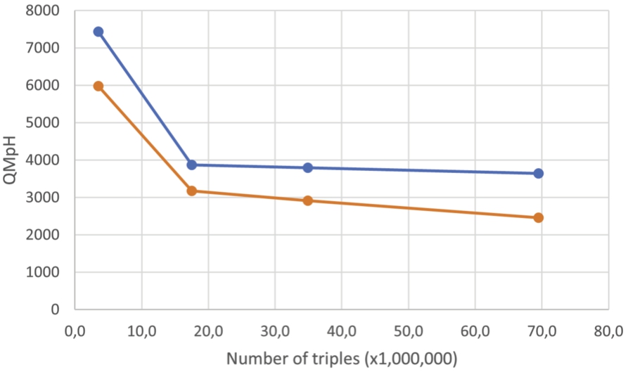
6.1.4.Merge time comparison
To test the efficiency of the merge step, we ran the BSBM update benchmark task using qEndpoint with 10k, 50k, 100k and 200K products, each with two different configurations. One using a high triples threshold of 1,000,000 triples, so our endpoint wasn’t running a merge process and one with a low threshold to force our endpoint to trigger merge operations during the experiment. We used a laptop with 16 GB of RAM and a 1TB SSD.
To decide the right threshold, we looked at the amount of changes for each query mix in the update experiment of the BSBM. This amount was of 1,000 changes for the 3.53M triples dataset and of 2,000 changes for the 69,5M triples dataset. We decided to choose a threshold of 1,000. Like this the system would constantly be in a merge state, allowing us to compare the worst case scenario (constantly merging) with the perfect case scenario (nearly no update, never merging). The count of merges was added as a second metric.
During the previous experiments we saw that the performance of the native store lack behind the qEndpoint. Also we saw that the mapped mode (versus the loaded mode) is more relevant since it allows to scale to bigger datasets. For these reasons we only indicate the results of the qEndpoint in mapping mode. We report the results in Table 3. In the results, we can see that the gap between an extensive amount of merges and no usage of the merge is negligible compared to the overall time of the benchmark. We can also notice that the number of merges is reduced with an increased datasets size. This can be explained by the time to run a merge which depends on the amount of data to merge, we explain this difference with the difference between the factor of runtime increase and triples increase. Where we have 5 times the count of triples from 3.53 to 17.5 with only 2 times the runtime. The merge processes are then longer, so we can’t fit as many in the new runtime.
Table 3
Merges comparison using BSBM update benchmark task
| # Triples | No merge | With merges | ||||
| QMpH | Merges | Runtime (s) | QMpH | Merges | Runtime (s) | |
| 3.53M | 7439 | 0 | 241 | 5982 | 13 | 300 |
| 17.5M | 3868 | 0 | 465 | 3180 | 8 | 565 |
| 34.9M | 3793 | 0 | 474 | 2912 | 4 | 617 |
| 69.5M | 3650 | 0 | 494 | 2456 | 4 | 732 |
6.2.WDBench
To compare qEndpoint with existing triple stores on a large KG, we decided to use the recent WDBench [3] benchmark, based on the real-world Wikidata77 RDF dataset and a selection of queries from the Wikidata query logs. WDBench is only using the “direct properties” of Wikidata, in other words, it is not containing reefied statements, leading to 1.2 billion triples. Due to that, it lacks analytical queries, but it is a good benchmark to compare queries with joins or paths. Something our main partition with HDT should be better.
To run our experiments, we used an AMD EPYC 7281 with 16 virtualized cores, 64 GB of RAM and a 100 GB HDD. The performances for the other systems, namely Blazegraph, Jena, Neo4j and Virtuoso are drawn from the paper [3], which rely on a similar machine in terms of per-thread rating of the CPU, disk type and available RAM.
First we indexed the WDBench dataset. Table 4 compares the index size for the different triple stores. As shown in Table 4, the index is from 3 to 5 times smaller for our system compared to the competitors which reflects the advantage  .
.
Table 4
Size of the different indexes
| Engine | NTriples | Jena | Neo4J | Virtuoso | Blazegraph | qEndpoint |
| Index size | 156 GB | 110 GB | 112 GB | 70 GB | 70 GB | 19.7 GB |
Thereafter we run each query provided by WDBench one. For each of them we check if an error occurs or a timeout, otherwise we measure the execution time. The timeout is set to 1 minute and is as in the WDBench paper, is considered when computing the average and median times. The queries are splitted into 5 types.
– Basic graph pattern (BGP) with two sub types: Single or Multiple
– Optional queries containing OPTIONAL fields
– Path queries
– Navigational graph patterns
Table 5
Results with the WDBench from the different types of queries for qEndpoint and our baseline, timeout = 60 s, result: best values
| Query type | Count | Engine | Error | Timeout | Average time (s) | Median time (s) |
| Single BGPs | 280 | Jena | 0 | 25 | 9.92 | 0.46 |
| Neo4J | 0 | 47 | 15.28 | 2.03 | ||
| Blazegraph | 0 | 3 | 1.73 | 0.07 | ||
| Virtuoso | 0 | 1 | 2.12 | 0.28 | ||
| qEndpoint | 0 | 0 | 0.53 | 0.02 | ||
| Multiple BGPs | 681 | Jena | 0 | 54 | 11.06 | 3.16 |
| Neo4J | 1 | 159 | 22.17 | 6.75 | ||
| Blazegraph | 0 | 52 | 8.47 | 1.34 | ||
| Virtuoso | 3 | 7 | 8.71 | 8.34 | ||
| qEndpoint | 0 | 10 | 3.21 | 1.54 | ||
| Optionals | 498 | Jena | 0 | 59 | 13.56 | 4.34 |
| Neo4J | 1 | 146 | 27.09 | 17.87 | ||
| Blazegraph | 0 | 37 | 8.55 | 2.2 | ||
| Virtuoso | 2 | 69 | 17.29 | 9.5 | ||
| qEndpoint | 0 | 4 | 2.31 | 1.6 | ||
| Path | 660 | Jena | 0 | 96 | 11.74 | 0.81 |
| Neo4J | 6 | 134 | 20.89 | 9.74 | ||
| Blazegraph | 0 | 87 | 11.00 | 0.82 | ||
| Virtuoso | 27 | 24 | 4.71 | 0.70 | ||
| qEndpoint | 0 | 17 | 2.33 | 0.43 | ||
| Navigational | 539 | Jena | 0 | 245 | 30.98 | 29.83 |
| Neo4J | 0 | 211 | 31.07 | 24.83 | ||
| Blazegraph | 0 | 180 | 22.32 | 2.58 | ||
| Virtuoso | 2 | 37 | 10.42 | 4.36 | ||
| qEndpoint | 0 | 51 | 8.73 | 0.97 |
We report the WDBench results in Table 5. We can see that as predicted, thanks to the main-partition, our system is faster to run most of the queries  . We can see that the query performance is at least 3 times faster on BGPs and at least 2 times faster on path, navigational and optional queries.
6.3.Indexing and querying Wikidata
In the following we describe how to index and query Wikidata as well as a comparison with existing alternatives.
6.3.1.Loading data
To load the full Wikidata dump into qEndpoint, one needs to run a few instructions. This is done using our indexing method to efficiently create the HDT partition (Point 1 in the Fig. 1)
With few commands, it allows everyone to quickly have a SPARQL endpoint over Wikidata without the need of special configurations. Note that the Wikidata dump is not uncompressed during this process. In particular, the disk footprint needed to generate the index is lower than the uncompressed dump (which is around 1.5 Tb). In the Table 6, we can see the time spent for the different indexing steps.
Table 6
Time split during the loading of the Wikidata dataset
| Task | Time | Description |
| Dataset download | 7 h | Download the dataset* |
| HDT compression | 45 h | Creating HDT |
| HDT co-index gen | 5 h | Creating OPS/PSO/POS indexes |
| Loading the index | 2 min | Start the endpoint |
* The time to download the dataset wasn’t taken into account in the 50 h.
Table 7
Wikidata index characteristics for different endpoints
| System | Loading Time | #Triples | RAM | Index size | Doc |
| Apache Jena | 9d 21 h | 13.8 B | 64 GB | 2TB | 1 |
| Virtuoso | several days*(preprocessing) + 10 h | 11.9 B | 378 GB | NA | 2 |
| Blazegraph | ∼5.5d | 11.9 B | 128 GB | 1.1 T | 3 |
| Stardog | 9.5 h | 16.7 B | 256 GB | NA | 4 |
| QLever | 14.3 h | 17 B | 128 GB | 823 GB | 5 |
| qEndpoint | 50 h | 17.4 B | 10 GB | 294 GB | 6 |
* The precise number of days for the preprocessing is not indicated in the documentation.
For comparison, to date, it exists only few attempts to successfully index Wikidata [10]. Since 2022, when the Wikidata dump exceeded 10B triples, only 4 triple stores are reported to be capable of indexing the whole dump, namely: Virtuoso [9], Apache Jena,88 QLever [4] and Blazegraph.
Virtuoso is a SQL based SPARQL engine where the changes on the RDF graph are reflected to a SQL database.
QLever is a SPARQL engine using an RDF custom binary format to index and compress RDF graphs. It supports a text search engine, but only the SPARQL engine will be compared during this experiment.
Blazegraph is a SPARQL engine using a B+Tree implementation to store the RDF graph, it is currently used by Wikidata.
Jena is a SPARQL engine also using a B+Tree implementation to store the RDF graph. Unlike Blazegraph the Jena’s implementation wasn’t considered for large RDF graph storage.
We report in Table 7 the loading times, the number of indexed triples, the amount of needed RAM, the final index size and the documentation for indexing Wikidata.
Overall, we can see that the qEndpoint has the lowest RAM footprint as well as the lowest disk footprint. Also, it offers an easy documentation for compressing the whole Wikidata dump. The time to index is the second best compared to the other systems. Most notably, the qEndpoint is the only setup that allows currently to index Wikidata on commodity hardware.
6.3.2.Loading a pre-computed index
Table 8
Sizes of each components of qEndpoint (total: 296 GB)
| File name | File size | Usage |
| index_dev.hdt | 183 GB | Dictionary + SPO index |
| index_dev.hdt.index.v1-1 | 113 GB | OPS/PSO/POS indexes |
| native-store | 16 KB | RDF4J store |
| qendpoint.jar | 82 MB | qEndpoint |
HDT is meant to be a format for sharing RDF datasets [13] and was therefore designed to have a particularly low disk footprint. Table 8 shows the sizes of the components needed to currently set up a Wikidata SPARQL endpoint using only HDT, which amounts to the first two rows in the table, i.e. 300 GB in total. The RDF4j counterpart, which is the third row in Table 8, corresponds to 16 KB. Compared with the other endpoints in Table 7, the whole data can be easily downloaded in a few hours with any high-speed internet connection.
The second component in Table 6 of 113 GB can be avoided in setups with slow connections since this co-index can be computed in 5 h. As a consequence, it is possible to further reduce the amount of time required to deploy a full SPARQL endpoint. This time turns to be shrunk to a few minutes after downloading the files in Table 6.99 Note that the whole bzip2 Wikidata dump is more than 150 GB.1010 This means that by sharing the index, the setup time can be reduced to the amount of time that is necessary to download double of the size of the plain compressed Wikidata dump.
6.3.3.Queries
In the following, we discuss the evaluation of the query performance of the qEndpoint with other available systems. To the best of our knowledge, ours is also the first evaluation on the whole Wikidata dump using historical query logs.
As described above, while there are successful attempts to set up a local Wikidata endpoint, these are difficult to reproduce and depending on the cases the needed hardware resources are difficult to find [10]. Therefore, in order to compare with existing systems, we restrict to those whose setups are publicly available:
– Blazegraph: the current system that is used in production by Wikimedia Foundation available at https://query.wikidata.org/sparql;
– Virtuoso: a live demo was set up in 20191111 that is available at https://wikidata.demo.openlinksw.com/sparql;
– QLever: a live demo is available at https://qlever.cs.uni-freiburg.de/wikidata and was set up in 2022.
1. No usage of http://www.bigdata.com/ functions, internal to Blazegraph and not supported by other endpoints
2. No MINUS operation, currently not supported by the qEndpoint.
Unlike with WDBench, the whole dataset is used, increasing the usage of analytic queries, our system being on commodity hardware, we except to have worse results for some query due to a lack of resources to compensate.
The resources for the compared systems are the same as the one reported for indexing in Table 7.
The Wikidata logs queries results are presented in Fig. 3 and Table 10.
Table 9
Query count per type
| Query type | Count |
| Triple Pattern (TP) | 5285 |
| Recursive / Path queries | 2852 |
| TP + Filter | 986 |
| TP + Union | 213 |
| Other | 664 |
Fig. 3.
qEndPoint time difference with 3 different endpoint (QLever, Virtuoso, Blazegraph from left to right) over 10K random queries without considering errors, one square is one query. A square is green if qEndPoint is faster and red if the baseline is faster. The intensity is based on the time difference which is between −6 and +6 seconds.
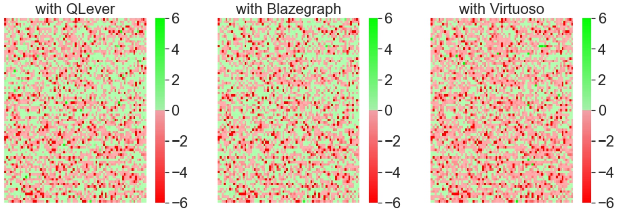
Table 10
Errors per endpoint on 10K random queries of the Wikidata query logs
| Endpoint | Parsing errors | Timeout errors | Evaluation errors |
| QLever | 4174 | 0 | 0 |
| Virtuoso | 146 | 1 | 0 |
| qEndpoint | 0 | 808 | 0 |
| Blazegraph | 0 | 10 | 1 |
We observe that the various systems have varying level of SPARQL support (see Table 10) and that qEndpoint via RDF4J can correctly parse all the queries. As shown in Table 11, it achieves better performances than QLever in 44% of the cases (despite 4x lower memory footprint). It outperforms Virtuoso in 34% of the cases (despite 10x lower memory footprint) and it outperforms Blazegraph (the production system used by Wikimedia Deutschland with Wikidata) in 46% of the cases (despite a 4x lower memory footprint). Overall, we see that the median execution time between the qEndpoint and the other systems is −0.05. This means that, modulo a few outliers, we can achieve comparable query speed with reduced memory and disk footprint. By manually investigating some queries, we believe that the outliers are due to query optimization problems that we plan to tackle in the future. For example by switching the order of the triple patterns in the query.
Overall, despite running on commodity hardware, qEndpoint can achieve query speeds comparable to other existing alternatives. The dataset and the scripts used for the experiments are available online.1313
6.4.Results
During the demonstration, we plan to show the following capabilities of qEndpoint:
– how it is possible to index Wikidata on a commodity hardware;
– how it is possible to set up a SPARQL endpoint by downloading a pre-computed index; (Point 2 in the Fig. 1)
– the performance of qEndpoint on typical queries over Wikidata from our test dataset (see Table 9). Query types that are relevant for showcasing are simple triple pattern queries (TP), TPs with Unions, TPs with filters, Recursive path queries and other query types found in the Wikidata query logs. We will also be able to load queries formulated by the visitors of our demo booth.
The objective is to demonstrate that the qEndpoint performance is overall comparable with the other endpoints despite the considerable lower hardware resources. As such, it represents a suitable alternative to current resource-intensive endpoints.
Table 11
Statistics over the time differences in seconds with the percentage of queries qEndpoint was faster. result: best values
| Endpoint | Max | Min | Mean | Median | % outperf. |
| QLever | 60 | −60.0 | −2.8 | −0.05 | 44.4 |
| Blazegraph | 4.74 | −60.0 | −2.8 | −0.04 | 45.9 |
| Virtuoso | 60.0 | −60.0 | −2.88 | −0.04 | 34.4 |
7.Usage in production
The above implementation is used in two projects that are in production and currently operational at the European Commission, the European Direct Contact Center (EDCC) and Kohesio.
7.1.European direct contact center
The European Direct Contact Center1414 (EDCC) is a contact center of the European Union receiving every year 200k messages from citizens with questions about the EU. The information used to answer questions are stored in the EDCC Knowledge Base (KB), a KG containing resources to help operators to answer the received questions.
7.2.Kohesio
Kohesio is an EU project that aims to make research projects funded by the EU discoverable by EU citizens (https://kohesio.ec.europa.eu/). Kohesio is constructed on top of the EU KG [7] (available at https://linkedopendata.eu), a graph describing the EU and containing its funded projects. The graph is hosted in a Wikibase instance and contains 726 million triples. All interactions of the Kohesio applications are converted into SPARQL queries that are running over the qEndpoint.1515
8.Supplemental material statement
The qEndpoint is implemented as a RDF4J Sail. The code of the qEndpoint is available on Github under https://github.com/the-qa-company/qEndpoint.
9.Conclusions
In this paper, we have presented the qEndpoint, a triple store that uses an architecture based on differential-updates. This represents the first graph database based on this architecture. We have presented: a) details about suitable data-structures that can be used for the main and delta partition respectively, b) a detail description of the merge process.
We have evaluated over different benchmarks the performance of the architecture as well as the efficiency of the implementation that we provided against other public endpoints. We see the following main advantages of this architecture: high read performance  , fast insert performance
  , fast delete performance
  , small index size
  , fast index speed
  , and good analytical performance
  .
.
These results show that the architecture that we propose is promising for graph databases. On the other side this is a first step towards graph databases with this architecture. Open challenges are for example:
– be able to query named graphs [14],
– exploit more the data structure of HDT to construct better query plans (for example, using merge joins instead of the current nested ones) and improve in OLAP scenarios,
– propose new versions of HDT optimized for querying (to support for example filters over numbers),
– propose a distributed version of the system
Notes
9 The index files are currently available at the URL https://qanswer-svc4.univ-st-etienne.fr/ into the RDF HDT open format.
References
[1] | D. Abadi, P.A. Boncz, S. Harizopoulos, S. Idreos and S. Madden, The design and implementation of modern column-oriented database systems, Found. Trends Databases 5: (3) ((2013) ), 197–280. doi:10.1561/1900000024. |
[2] | W. Ali, M. Saleem, B. Yao, A. Hogan and A.-C.N. Ngomo, Storage, indexing, query processing, and benchmarking in centralized and distributed RDF engines: a survey, (2020) . |
[3] | R. Angles, C.B. Aranda, A. Hogan, C. Rojas and D. Vrgoč, WDBench: A Wikidata graph query benchmark, in: The Semantic Web–ISWC 2022: 21st International Semantic Web Conference, Virtual Event, October 23–27, 2022, Proceedings, Springer, (2022) , pp. 714–731. doi:10.1007/978-3-031-19433-7_41. |
[4] | H. Bast and B. Buchhold, Qlever: A query engine for efficient sparql+ text search, in: Proceedings of the 2017 ACM on Conference on Information and Knowledge Management, (2017) , pp. 647–656. doi:10.1145/3132847.3132921. |
[5] | C. Bizer and A. Schultz, The Berlin sparql benchmark, International Journal on Semantic Web and Information Systems (IJSWIS) 5: (2) ((2009) ), 1–24. doi:10.4018/jswis.2009040101. |
[6] | D. Diefenbach and J.M. Giménez-García, HDTCat: Let’s make HDT generation scale, in: International Semantic Web Conference, Springer, (2020) , pp. 18–33. |
[7] | D. Diefenbach, M.D. Wilde and S. Alipio, Wikibase as an infrastructure for knowledge graphs: The eu knowledge graph, in: The Semantic Web–ISWC 2021: 20th International Semantic Web Conference, ISWC 2021, Virtual Event, October 24–28, 2021, Proceedings 20, Springer, (2021) , pp. 631–647. doi:10.1007/978-3-030-88361-4_37. |
[8] | L. Duroyon, F. Goasdoué, I. Manolescu, F. Goasdoué and I. Manolescu, A linked data model for facts, statements and beliefs, in: Companion Proceedings of the 2019 World Wide Web Conference, (2019) , pp. 988–993. doi:10.1145/3308560.3316737. |
[9] | O. Erling and I. Mikhailov, in: RDF Support in the Virtuoso DBMS, Networked Knowledge-Networked Media: Integrating Knowledge Management, New Media Technologies and Semantic Systems, (2009) , pp. 7–24. doi:10.1007/978-3-642-02184-8_2. |
[10] | W. Fahl, T. Holzheim, A. Westerinen, C. Lange and S. Decker, Getting and hosting your own copy of Wikidata, in: 3rd Wikidata Workshop @ International Semantic Web Conference, (2022) , https://zenodo.org/record/7185889#.Y0WD1y0RoQ0. |
[11] | F. Färber, N. May, W. Lehner, P. Große, I. Müller, H. Rauhe and J. Dees, The SAP HANA database–an architecture overview, IEEE Data Eng. Bull. 35: (1) ((2012) ), 28–33. |
[12] | J.D. Fernández, M.A. Martínez-Prieto, C. Gutiérrez, A. Polleres and M. Arias, Binary RDF representation for publication and exchange (HDT), Journal of Web Semantics 19: ((2013) ), 22–41. doi:10.1016/j.websem.2013.01.002. |
[13] | J.D. Fernandez, M.A. Martınez-Prieto, C. Gutierrez, A. Polleres and M. Arias, Binary RDF Representation for Publication and Exchange (HDT) ((2013) ). |
[14] | J.D. Fernández, M.A. Martínez-Prieto, A. Polleres and J. Reindorf, HDTQ: Managing RDF datasets in compressed space, in: European Semantic Web Conference, Springer, (2018) , pp. 191–208. doi:10.1007/978-3-319-93417-4_13. |
[15] | J. Giceva and M. Sadoghi, Hybrid OLTP and OLAP, in: Encyclopedia of Big Data Technologies, S. Sakr and A.Y. Zomaya, eds, Springer, (2019) . |
[16] | M. Hwang, in: Graph Processing Using SAP HANA: A Teaching Case., E-Journal of Business Education and Scholarship of Teaching, Vol. 12: , (2018) , pp. 155–165. |
[17] | J. Krueger, M. Grund, C. Tinnefeld, H. Plattner, A. Zeier and F. Faerber, Optimizing write performance for read optimized databases, in: International Conference on Database Systems for Advanced Applications, Springer, (2010) , pp. 291–305. doi:10.1007/978-3-642-12098-5_23. |
[18] | J. Krueger, C. Kim, M. Grund, N. Satish, D. Schwalb, J. Chhugani, H. Plattner, P. Dubey and A. Zeier, Fast updates on read-optimized databases using multi-core CPUs, (2011) , arXiv preprint arXiv:1109.6885. |
[19] | S. Malyshev, M. Krötzsch, L. González, J. Gonsior and A. Bielefeldt, Getting the most out of Wikidata: Semantic technology usage in Wikipedia’s knowledge graph, in: International Semantic Web Conference, Springer, (2018) , pp. 376–394. |
[20] | M.A. Martínez-Prieto, M. Arias Gallego and J.D. Fernández, Exchange and consumption of huge RDF data, in: Extended Semantic Web Conference, Springer, (2012) , pp. 437–452. |
[21] | T. Neumann and G. Weikum, RDF-3X: A RISC-style engine for RDF, Proceedings of the VLDB Endowment 1: (1) ((2008) ), 647–659. doi:10.14778/1453856.1453927. |
[22] | T. Neumann and G. Weikum, x-RDF-3X: Fast querying, high update rates, and consistency for RDF databases, Proceedings of the VLDB Endowment 3: (1–2) ((2010) ), 256–263. doi:10.14778/1920841.1920877. |
[23] | qEndpoint, Benchmark values, (2023) . |
[24] | S. Sakr, A. Bonifati, H. Voigt, A. Iosup, K. Ammar, R. Angles, W.G. Aref, M. Arenas, M. Besta, P.A. Boncz, K. Daudjee, E.D. Valle, S. Dumbrava, O. Hartig, B. Haslhofer, T. Hegeman, J. Hidders, K. Hose, A. Iamnitchi, V. Kalavri, H. Kapp, W. Martens, M.T. Özsu, E. Peukert, S. Plantikow, M. Ragab, M. Ripeanu, S. Salihoglu, C. Schulz, P. Selmer, J.F. Sequeda, J. Shinavier, G. Szárnyas, R. Tommasini, A. Tumeo, A. Uta, A.L. Varbanescu, H. Wu, N. Yakovets, D. Yan and E. Yoneki, The future is big graphs: A community view on graph processing systems, Commun. ACM 64: (9) ((2021) ), 62–71. doi:10.1145/3434642. |
[25] | M. Stonebraker, D.J. Abadi, A. Batkin, X. Chen, M. Cherniack, M. Ferreira, E. Lau, A. Lin, S. Madden, E. O’Neil, P. O’Neil, A. Rasin, N. Tran and S. Zdonik, C-Store: A Column-Oriented DBMS, in: Making Databases Work: The Pragmatic Wisdom of Michael Stonebraker, Association for Computing Machinery and Morgan Claypool, (2018) , pp. 491–518. ISBN 9781947487192. doi:10.1145/3226595.3226638. |
[26] | R. Taelman, M. Vander Sande and R. Verborgh, OSTRICH: Versioned random-access triple store, in: Companion Proceedings of the Web Conference 2018, (2018) , pp. 127–130. |
[27] | J. Webber, A Programmatic Introduction to Neo4j, in: Proceedings of the 3rd Annual Conference on Systems, Programming, and Applications: Software for Humanity, SPLASH ’12, Association for Computing Machinery, New York, NY, USA, (2012) , pp. 217–218. ISBN 9781450315630. doi:10.1145/2384716.2384777. |
[28] | K. Wilkinson and K. Wilkinson, Jena property table implementation, Ssws ((2006) ). |
[29] | K. Zeng, J. Yang, H. Wang, B. Shao and Z. Wang, A distributed graph engine for web scale RDF data, Proceedings of the VLDB Endowment 6: (4) ((2013) ), 265–276. doi:10.14778/2535570.2488333. |


