
Ontology-based GraphQL server generation for data access and data integration
Abstract
In a GraphQL Web API, a so-called GraphQL schema defines the types of data objects that can be queried, and so-called resolver functions are responsible for fetching the relevant data from underlying data sources. Thus, we can expect to use GraphQL not only for data access but also for data integration, if the GraphQL schema reflects the semantics of data from multiple data sources, and the resolver functions can obtain data from these data sources and structure the data according to the schema. However, there does not exist a semantics-aware approach to employ GraphQL for data integration. Furthermore, there are no formal methods for defining a GraphQL API based on an ontology. In this work, we introduce a framework for using GraphQL in which a global domain ontology informs the generation of a GraphQL server that answers requests by querying heterogeneous data sources. The core of this framework consists of an algorithm to generate a GraphQL schema based on an ontology and a generic resolver function based on semantic mappings. We provide a prototype, OBG-gen, of this framework, and we evaluate our approach over a real-world data integration scenario in the materials design domain and two synthetic benchmark scenarios (Linköping GraphQL Benchmark and GTFS-Madrid-Bench). The experimental results of our evaluation indicate that: (i) our approach is feasible to generate GraphQL servers for data access and integration over heterogeneous data sources, thus avoiding a manual construction of GraphQL servers, and (ii) our data access and integration approach is general and applicable to different domains where data is shared or queried via different ways.
1.Introduction
GraphQL is a conceptual framework to build APIs for Web and mobile applications [29]. It was publicly released by Facebook in 2015 and, since then, the GraphQL ecosystem11 has grown tremendously in terms of libraries22 supporting different programming languages (such as Python, Java and JavaScript), tools (such as Apollo and GraphiQL), and adopters (such as Airbnb, IBM and Twitter). The framework introduces the notion of a schema. Such a schema of a GraphQL API contains type definitions which specify what data objects can be retrieved from the API. The framework also contains a form of query language for expressing such data retrieval requests. A third component of GraphQL are resolver functions, which are typically used for executing GraphQL queries in a GraphQL server. That is, such resolvers specify – in terms of program code – how data related to the various elements of a GraphQL schema has to be fetched from underlying data sources.33
GraphQL could be used to integrate data from different data sources by building a GraphQL server over these sources, in which the GraphQL schema provides a view over data from multiple sources, and the resolver functions contain implementations for accessing multiple sources. However, a semantics-aware approach to employing GraphQL for data integration does not exist. The approaches in [11] and [4] introduce how to use GraphQL for data federation. The semantics of data are not explicit in a machine-processable form which means the developer needs to write program code (i.e., resolver functions) to populate the various elements of a GraphQL schema. Furthermore, there are no formal methods for defining a GraphQL schema. The developers have to define a GraphQL schema manually. The aim of this work is to provide a semantics-aware approach to employ GraphQL for data integration, with formal methods to generate the GraphQL server.
Research problem: This article focuses on the following question: How can ontologies be leveraged to generate GraphQL APIs for semantics-aware data access and data integration? We pursue the objectives: (i) to provide an ontology-driven data access and integration approach in which a GraphQL server accesses underlying data sources by providing an integrated view of the data; (ii) to formally generate GraphQL servers automatically to avoid manual constructions of the servers.
Contributions: To address the research question, we propose a framework for GraphQL-based data access and integration in which an ontology drives the generation of a GraphQL server.44 More specifically, given an ontology as an integrated view of data from multiple data sources, the first contribution is that we propose and implement a method for generating a GraphQL schema based on semantic assets in this ontology such that the schema becomes a view of the data to be integrated. Then, the second contribution is that we introduce a generic approach to create a GraphQL server that is capable to get data from the corresponding data sources by relying on semantic mappings that use the ontology.
The remainder of the article is organized as follows. We provide the relevant background regarding ontologies, description logics, data integration and GraphQL in Section 2. Then we outline the proposed GraphQL-based framework in Section 3 and elaborate on the implementation of this framework in Sections 4 and 5. Section 6 introduces related work. Section 7 presents an evaluation based on a real-world data integration scenario in the materials design domain and evaluations based on two synthetic benchmark scenarios, the Linköping GraphQL Benchmark (LinGBM) and GTFS-Madrid-Bench. Section 8 discusses the strengths and limitations of our approach, and introduces the directions for future work. Finally in Section 9, we present concluding remarks.
2.Background
This section provides background information on ontologies, description logics, data integration and GraphQL.
2.1.Ontologies and description logics
The term ontology originates in philosophy, in which it is the science of what is, of the kinds and structures of objects, properties, and relationships in every area of reality [57,64]. Ontologies can be viewed, intuitively, as defining the terms, relations, and rules that combine these terms and relations in a domain of interest [59]. Through ontologies, people and organizations are able to communicate by establishing a common terminology. They provide the basis for interoperability between systems and are applicable as an index to a repository of information as well as a query model and a navigation model for data sources. Moreover, they are often used as a foundation for integrating data sources, thereby alleviating the heterogeneity issue. The benefits of using ontologies are their improved reusability, share-ability and portability across platforms, as well as their increased maintainability and reliability. On the whole, ontologies allow a field to be better understood and allow information in that field to be handled much more effectively and efficiently (e.g., knowledge representation for bioinformatics discussed in [58]).
Fig. 1.
Example of an ontology of the university domain including 4 concepts and relationships among them, as well as relationships between concepts and datatypes.
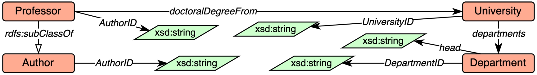
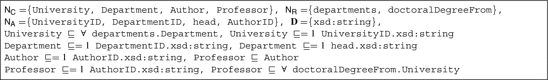
From a knowledge representation point of view, ontologies usually contain four components: (i) concepts that represent sets or classes of entities in a domain, (ii) instances that represent the actual entities, (iii) relations, and (iv) axioms that represent facts that are always true in the topic area of the ontology. Relations represent relationships among concepts. Axioms represent domain restrictions, cardinality restrictions, or disjointness restrictions. Depending on the components and information related to the components they contain, ontologies can be classified. Figure 1 represents an example ontology for the university domain. The open-headed arrows represent axioms that represent is-a relationships that is, if A is a B, then all entities belonging to concept A also belong to concept B. We say that A is a sub-concept of B. In this example Professor is a sub-concept of Author. Therefore, all Professor entities are Author entities. The closed-headed arrows represent general relations among concepts other than is-a relations. For instance, the Professor concept has a connection to the University concept represented by the doctoralDegreeFrom relation. Additionally, a relation can exist between a concept and a data type reference. For instance, University has a connection to the data type reference xsd:string represented by the UniversityID relation. This means that each entity of the University concept can be associated with a string type value by having a UniversityID connection.
To formally define the above concepts and relationships, we need representation languages. Description logics (DL) are a family of knowledge representation languages. There are three basic building blocks of such a language, namely: (i) atomic concepts (unary predicates) such as University and Department, (ii) atomic roles (binary predicates) such as departments, and (iii) individuals (constants) [7]. Complex concepts and roles can be built by using atomic concepts and logical constructors (e.g., conjunction (⊓), disjunction (⊔), universal restriction (∀) and existential restriction (∃)). Axioms can be defined using general concept inclusions (⊑). For instance, the general concept inclusion (GCI)
2.2.Data integration
Data integration deals with combining data that resides at multiple different sources [14,26,43]. Ideally, a data integration system should enable unified access to a number of data sources [26,43]. Formally, according to [43], a data integration system can be formalized as a triple
–
–
–
Ontology-based data integration (OBDI) is a form of data integration in which an ontology plays the role of a global schema that captures domain knowledge [15]. Usually, in an information system with only one single data source, the formal treatment of OBDI is identical to that of ontology-based data access (OBDA) [15,67]. In this article, we generally refer to both OBDI and OBDA as OBDA. OBDA, as a semantic technology, aims to facilitate access to different underlying data sources [66]. Traditionally, these underlying data sources are considered to be relational databases. Ontologies play the role of global views over multiple data sources. There are different ways to implement an OBDA system. Generally, these systems can be categorized into two types, namely, data warehouse-based approaches and virtual approaches. These two categories of methods both make use of semantic mappings in order to overcome the differences between ontologies and local schemas, but in different ways [21,65]. In a data warehouse-based approach, data from multiple sources are usually loaded or stored in a centralized storage, which is the warehouse [26,63], based on semantic mappings. We refer to the data in such warehouses as materialized data. Depending on the aims or functionalities of a system, the materialized data could be stored in local databases or transformed into RDF graphs. Therefore, queries are evaluated against the materialized data. In a virtual approach, data is retained at the original sources and mediators are used to translate queries defined in terms of a global or mediated schema into queries defined in terms of each data source’s local schema, based on semantic mappings. Therefore, queries are evaluated and executed against each data source. SPARQL queries are widely supported by data integration systems that use ontologies as global schemas.
A number of semantic mapping definition languages have been proposed over the years. One such language is R2RML (RDB to RDF Mapping Language),55 one of the two recommendations by the RDB2RDF W3C Working Group66 to define semantic mappings [22]. It supports transformation rules defined by users, while the other recommendation, Direct Mapping [5], does not. Another language is RDF Mapping Language (RML) [24,25], which allows underlying data in formats beyond relational databases and is a superset of R2RML. RML allows data from CSV, JSON, and XML data sources. In our work we make use of RML and we introduce RML in more details in Section 5.2.
2.3.GraphQL
GraphQL schemas and GraphQL resolver functions are basic building blocks in the implementations of GraphQL servers. The former describe how users can retrieve data using GraphQL APIs. The latter contain program code including how to access data sources and structure the obtained data according to the schema. We introduce GraphQL schemas and GraphQL resolver functions in Section 2.3.1 and Section 2.3.2, respectively.
2.3.1.GraphQL schemas
In a GraphQL API, the GraphQL schema defines types, their fields, and the value types of the fields. Such a schema represents a form of vocabulary supported by a GraphQL API rather than specifying what the data instances of an underlying data source may look like and what constraints have to be guaranteed [33]. There are six different (named) type definitions in GraphQL, which are scalar type, object type, interface type, union type, enum type and input object type. Listing 1 depicts a GraphQL schema example.
Listing 1.
Example of a GraphQL schema of the university domain
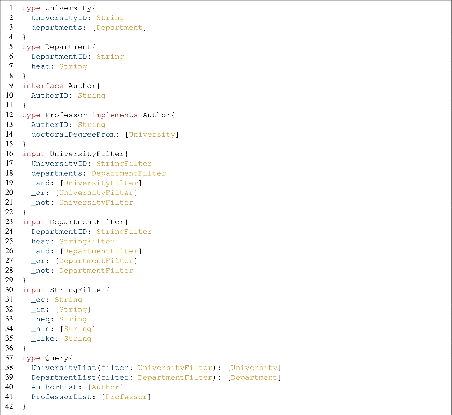
An object type represents a list of fields and each field has a value of a specific type such as object type or scalar type. A scalar is used to represent a value such as a string. In Listing 1, there are three basic object type definitions, which are University (line 1 to line 4), Department (line 5 to line 8), and Professor (line 12 to line 15). They all have field definitions which represent the relationships to scalar types or to other object types. For instance, the University type has a field definition UniversityID of which the value type is String (line 2), and a field definition departments of which the value type is a list of Departments (line 3). GraphQL allows defining abstract types by supporting the interface type and the union type. An interface type defines a list of fields and allows object types to implement. An object type can then implement an interface type with the requirement that the object type includes all fields defined by the interface type. The schema in Listing 1 contains an interface type, Author with an AuthorID field of which the value type is String (line 9 to line 11). The object type Professor implements Author and must have the same definition for AuthorID field (line 13) as that in Author. A union type defines a list of possible types. An enum type describes the set of possible values that are in scalars. For more details of union and enum types, we refer the reader to the latest GraphQL specification in [29].
GraphQL allows fields to accept arguments to configure their behavior [29]. These arguments can be defined by input object types. An input object type defines an input object with a set of input fields; the input fields are either scalars, enums, or other input objects. This allows arguments to accept arbitrarily complex structs, which can capture notions of filtering conditions. For instance, according to the definitions of UniversityFilter (line 16 to line 22) and StringFilter (line 30 to line 36), we can define an input argument as UniversityID:{_eq:”u1”} to capture the meaning of “UniversityID is equal to ‘u1’”, where _eq represents the equal to operator. In our approach, _and, _or and _not are used to represent boolean expressions. For instance, _or:[{UniversityID:{_eq:”u1”}},{UniversityID:{_eq:”u2”}}] represents the expression “UniversityID is equal to ‘u1’ or ‘u2’”. In the example schema, we use the term filter to represent the name of an input argument (e.g., line 38). Such input arguments defined as input objects are not built-in constructs of GraphQL. Therefore, their meanings are essentially defined by the program code of the GraphQL server implementation, i.e., the resolver functions which manage requests to underlying data sources and structure the returned data according to the GraphQL schema. Our approach presented in Section 4 and Section 5 uses input arguments named as filter to represent filter conditions.
Additionally, a GraphQL schema supports defining types that represent operations such as query and mutation. The schema presumes the Query type as the query root operation type. As Listing 1 shows, in the Query type definition (line 37 to line 42), there are four field definitions, which are UniversityList, DepartmentList, AuthorList, and ProfessorList. For instance, the returned type of UniversityList is [University], a list of Universities. The UniversityList takes an argument defined as UniversityFilter as an input for capturing the notion of a filtering condition.
2.3.2.GraphQL resolver functions
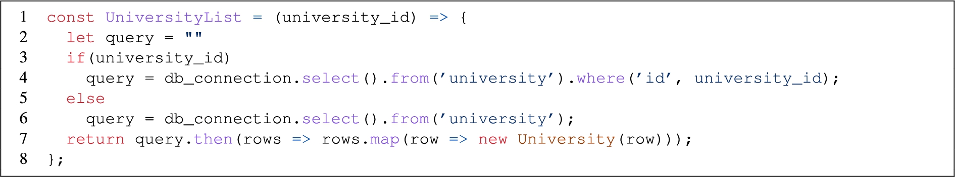
In a GraphQL API, apart from the GraphQL schema defining types, their fields, and the value types of the fields, resolver functions are responsible for populating the data for fields of types in the GraphQL schema. For instance, for the schema example shown in Listing 1, there are four fields defined in the Query type. Therefore, in the GraphQL server implementation, we are supposed to define resolver functions to populate data for these fields, UniversityList, DepartmentList, AuthorList, and ProfessorList. In our approach, we assume that the GraphQL schema supports a query that retrieves all the instances for each interface type or object type. Therefore, we use the name of each interface type or object type concatenated with ‘List’ as the name of a field in the Query type, where the returned type is a list of the interface or object type. This is a way to state the behavior of a field in the Query type. We emphasize that what a GraphQL query can retrieve over the underlying data sources relies on how the resolver function is implemented. For instance, if the underlying data source is a relational database, the resolver function should contain code specifying the SQL query to be evaluated. Listing 2 illustrates an example resolver function (written in JavaScript syntax) for the UniversityList field. We assume that the underlying data source is a relational database that contains a table named university with a column named id. In line 4, given an input argument (university_id) representing the id of a university, a query is evaluated against the relational database. In line 7, the data is structured according to the University object defined in the JavaScript code which corresponds to the University type definition in the schema shown in Listing 1.
Listing 2.
Example of a resolver function for the UniversityList field
3.GraphQL-based framework for data access and data integration
This section introduces an overview of the GraphQL-based framework for data access and integration and two basic processes in this framework.
3.1.Overview of the framework
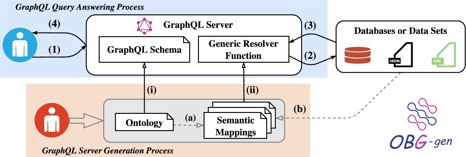
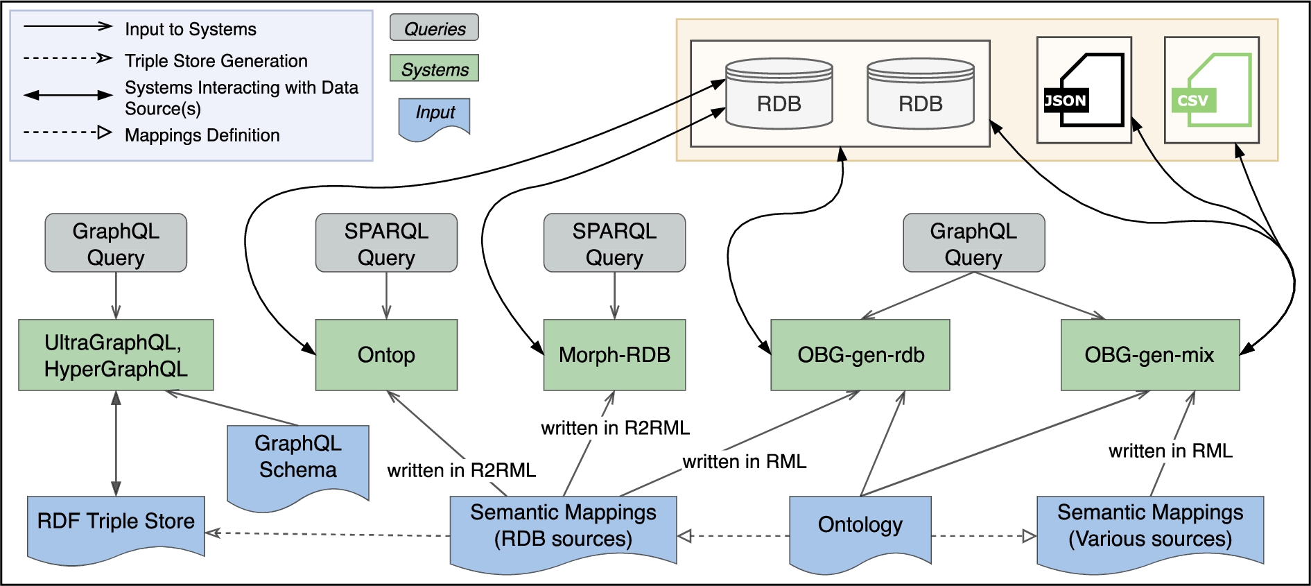
Figure 2 illustrates the framework for data access and integration based on GraphQL in which an ontology drives the generation of GraphQL server that provides integrated access to data from heterogeneous data sources. These data sources may be based on different schemas and formats and may be accessed in different ways (e.g., as tabular data accessed via SQL queries or as JSON-formatted data accessed via API requests). To address the heterogeneity, the framework relies on an ontology that provides an integrated view of the data from the different sources, and corresponding semantic mappings that define how the data from the underlying data sources is interpreted or annotated by the ontology (arrows (a) and (b)). Furthermore, two processes are defined. The first process generates the GraphQL server. The second process deals with answering queries and is performed after the GraphQL server is set up. In accordance with these two processes, there are two types of intended users or developers in the framework. One type is users or developers of the GraphQL server generator, who should have prior knowledge of the ontology, semantic mappings and the domain. The other type is end users using a GraphQL server for data access and integration, who may or may not be familiar with the Semantic Web or ontologies. For the purpose of writing GraphQL queries, they need basic prior knowledge of GraphQL, which can be learned from the self-documenting API of the generated GraphQL server showing the schema. We introduce more details about these two processes in Section 3.2 and Section 3.3, respectively.
Fig. 2.
GraphQL-based framework for data access and integration.
3.2.GraphQL server generation process
This process includes generating both a GraphQL schema for the API provided by the server (arrow (i)) and a generic resolver function (arrow (ii)). Given an ontology as an integrated view of data from multiple data sources, we propose a method for generating a GraphQL schema based on this ontology, with the result that the schema becomes a view of the data to be integrated. Additionally, we propose a generic implementation of resolver functions that takes semantic mappings as inputs, so that the server is able to get data from underlying data sources. In Sections 4 and 5, we elaborate on the implementation of our approaches for generating a GraphQL schema and the generic resolver function, respectively. This GraphQL server generation process does not need to be repeated unless the ontology or the semantic mappings change. After this generation process, the GraphQL server can be set up.
This process requires users or developers who are familiar with the query mechanisms of underlying data sources, domain ontologies that can be used for data access or integration. Consequently, they can define the scope of the ontology that will be used for generating the GraphQL schema for the server, as well as the semantic mappings that will be used for generating the generic resolver function. This type of automatic generation of GraphQL servers based on ontologies and semantic mappings can also benefit general GraphQL application developers, since it can eliminate the need to build GraphQL servers from scratch.
3.3.GraphQL query answering process
During this process the query is validated against the GraphQL schema (arrow (1)); the underlying data sources are accessed via resolver functions, the retrieved data is combined, the data is structured according to the schema (arrows (2) and (3)); and finally the query result is returned (arrow (4)).
Listing 3.
Example of a GraphQL query
Listing 4.
Example of a GraphQL query response
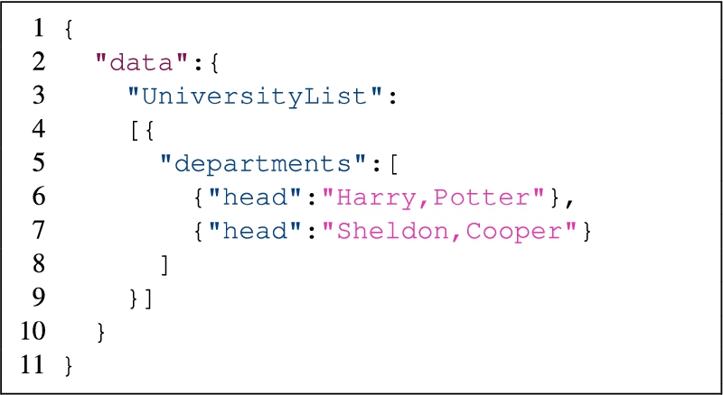
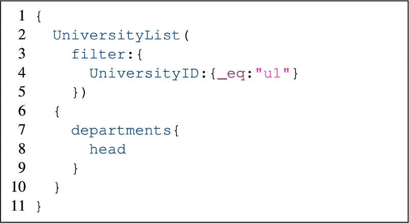
A GraphQL query example and corresponding query result are shown in Listing 3 and Listing 4, respectively. The example query is: “Get the university including the head of each department where the UniversityID is ‘u1’”. The query takes as an input an argument defined as filter:{UniversityID:{_eq:”u1”}}, which follows the syntax of the input object type UniversityFilter. As mentioned in Section 2.3.1, the meaning of an input argument defined as an input object type is essentially determined by the program code of the resolver functions. Thus the query example shown in Listing 3 illustrates one way that we make use of input objects to represent filtering conditions. In general, however, the input object types can be used in various ways for any field, depending on the implementation of the GraphQL server.
As mentioned earlier, domain users are the intended users of GraphQL servers, regardless of whether they have prior knowledge of the Semantic Web or ontologies. In order to write GraphQL queries, they only need to have a basic understanding of GraphQL, which can easily be explored via the GraphQL API provided by the server.
4.Ontology-based GraphQL schema generation
As mentioned in Section 2.3.1, the GraphQL schema represents a form of vocabulary supported by the GraphQL API rather than specifying what the data instances of an underlying data source may look like and what constraints have to be guaranteed. Therefore, we focus on GraphQL language features supporting semantics-aware and integrated data access, namely how data can be queried, rather than reflecting the semantics of a complex knowledge representation language in the context of a GraphQL schema. Section 4.1 introduces how a GraphQL schema is formalized, and Section 4.2 introduces how an ontology is represented via a description logic TBox. Given an ontology represented in a description logic TBox, the concept and role names can be used to generate types and fields in a GraphQL schema. The general concept inclusions in a description logic TBox can be used to specify how to connect generated types and fields in a GraphQL schema. Then, in Section 4.3, we present the core algorithm (Schema Generator) for generating a GraphQL schema based on an ontology. In Section 4.4, we present the intended meaning of GraphQL schemas generated by the Schema Generator.
4.1.GraphQL schema formalization
According to [33,34], a GraphQL schema can be defined over five finite sets. These five sets are
–
∗
∗
–
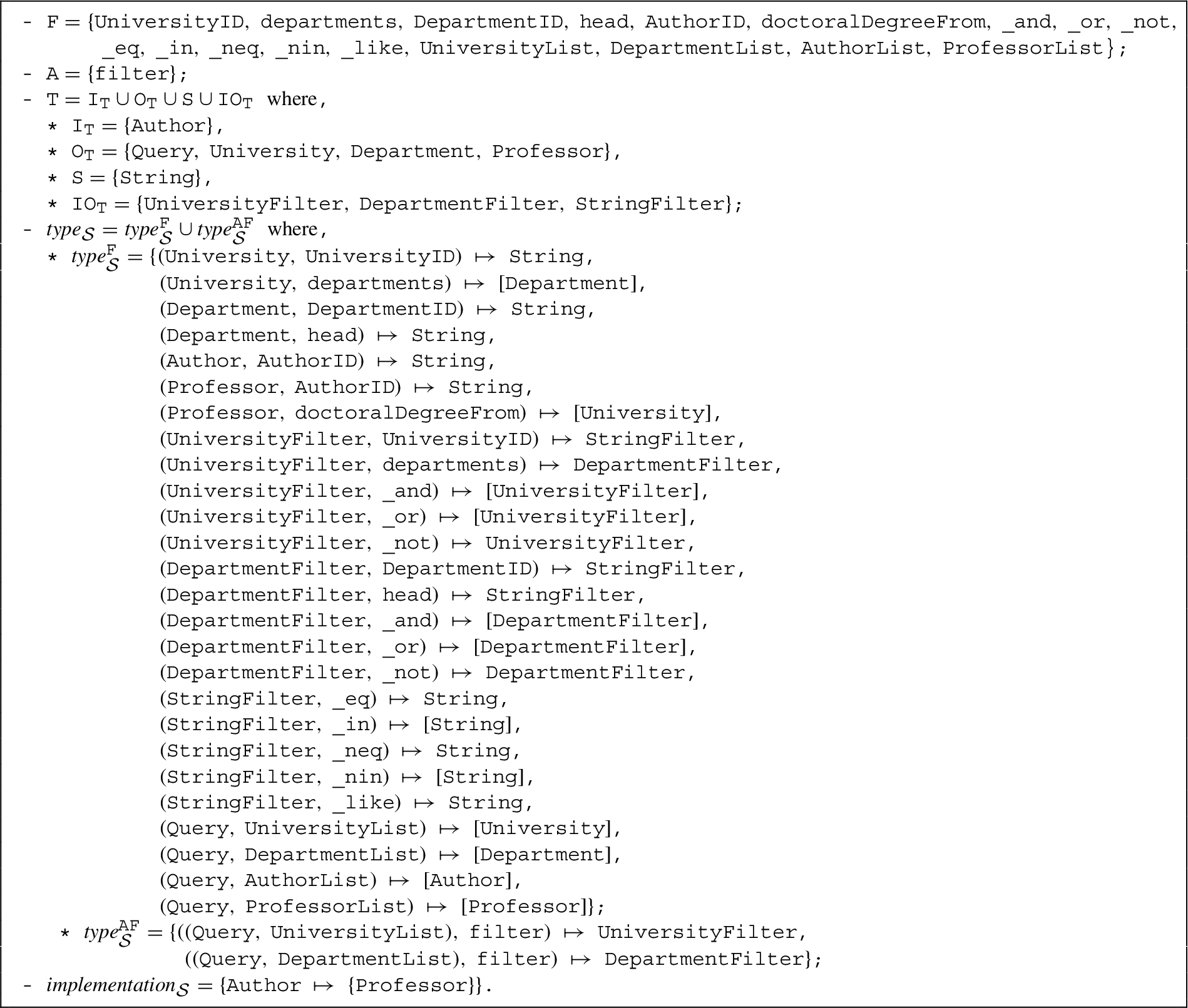
Listing 5 illustrates a formalized representation of the GraphQL schema shown in Listing 1. In the formalization, we have sets
4.2.Ontology representation by a description logic TBox
In this work we assume that the ontology is represented by a TBox in a description logic which is an extension of
Table 1
The syntax and semantics for the description logic used in our approach
| Name | Syntax | Semantics | |
| Construct | Top concept | ⊤ | |
| Atomic concept | P | ||
| Role | R | ||
| Attribute | A | ||
| Datatype | d | ||
| Conjunction | |||
| Role value restriction | |||
| Role qualified number restriction | |||
| Attribute value restriction | |||
| Attribute qualified number restriction | |||
| TBox | GCI | ||
| ABox | Concept assertion | ||
| Role assertion | |||
| Attribute assertion |
The syntax and semantics of the description logic used in our approach are shown in Table 1. The introduction of datatypes is based on the work presented in [35] and [36]. Let
A TBox over
4.3.Schema Generator algorithm
Algorithm 1 shows the details to generate a GraphQL schema. The output for the example is the schema shown in Listing 1. First, the algorithm iterates over the concept names in
From line 13 to line 21, the algorithm deals with GCIs containing roles, which can be of the form
We define a function Φ for mapping a datatype that exists in the TBox to a scalar type in GraphQL. Due to the fact that current GraphQL supports five basic scalar types which are ID, Float, Int, Boolean, and String, our current implementation of function Φ focuses on mapping datatypes xsd:float, xsd:int, xsd:string and xsd:boolean to scalar types Float, Int, String and Boolean, respectively. However, GraphQL allows users to define custom scalar types, and the values of such custom types should be JSON serializable. Therefore, our Φ function can be extended in the future for mapping any datatype besides the above four types from a TBox into a custom scalar type in GraphQL.
By generating the GraphQL schema based on an ontology, the schema will contain object or interface types corresponding to concepts in the ontology, and field declarations corresponding to relationships in the ontology. When a GraphQL query is sent to the GraphQL server, a resolver function parses the query to determine which type in the schema is requested. It then parses the relevant definitions corresponding to such a type in the semantic mappings to retrieve data. For instance, if a query requests all the entities of the University object type, the resolver function parses the semantic mappings that are defined for the University concept to get information regarding how to access the underlying data sources. 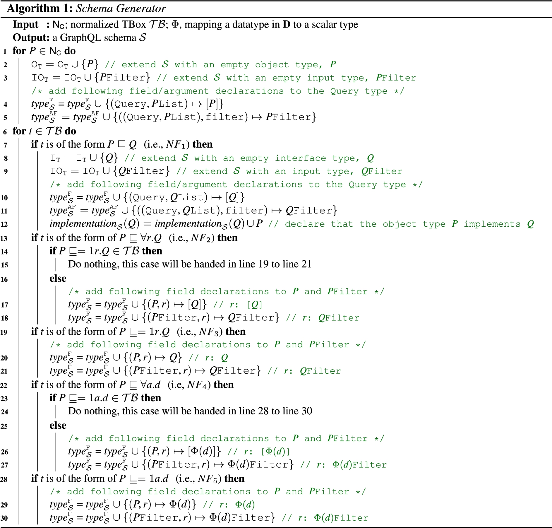
4.4.The intended meaning of a generated GraphQL schema
In Section 4.3, we present the Schema Generator which takes a TBox representing an ontology as an input, to generate a GraphQL schema. Such a GraphQL schema can describe how to access underlying data sources in which the data can be annotated by the ontology. The underlying data can thus be viewed as an ABox for the TBox. Therefore, a GraphQL query that conforms to this GraphQL schema can be considered as a query over the ABox. To make this intention more formal we consider an ABox
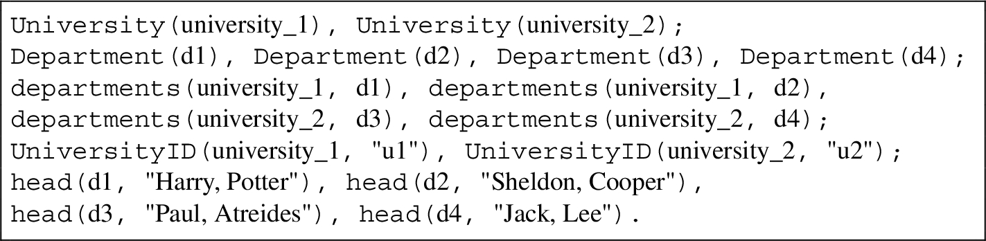
Let
– If
– If
For instance, given the query (as shown in Listing 3) and the above ABox, University(university_1), departments(university_1, d1), departments(university_1, d2), head(d1, “Harry, Potter”), head(d2, “Sheldon, Cooper”) are supposed to be retrieved. The above definition presents the meaning of the GraphQL schema generated based on a TBox for evaluating GraphQL queries. The definition relies on the Schema Generator where for each concept, the algorithm creates a corresponding type with the same name of the concept, same for roles and attributes. This guarantees to find the corresponding assertions from the ABox. However, in practice, as we presented in Section 2.3.2, how a GraphQL query retrieves data over the underlying data sources, depends on how the resolver function is implemented when we construct GraphQL servers. In the next section, we present how resolver functions can be implemented in a generic way based on semantic mappings.
5.Generic GraphQL resolver function
In general, there are two styles for implementing resolver functions for a GraphQL server. One option is to implement one resolver function per type (object or interface) defined in the GraphQL schema, where such a function states how to fetch the data to populate relevant fields. For instance, since the Query type in Listing 1 has four field definitions (UniversityList, DepartmentList, AuthorList, and ProfessorList), we may provide four resolver functions for getting entities of the University, Department, Author and Professor types from underlying data sources, respectively. The other option is to provide a resolver function for every field of every type defined in the GraphQL schema, such that this resolver could return data for this field of any type. In our framework, we adopt the first style because it can be easily generalized based on semantic mappings. That is, we implement a generic resolver function that can be used to populate objects of any object type or interface type, and can be viewed as a built-in function of the GraphQL server. In Section 5.1, we introduce how a GraphQL query is represented by Abstract Syntax Trees (ASTs), in which one represents query fields and others represent the filter expression. Section 5.2 introduces the RDF Mapping Language (RML), which is used for representing semantic mappings, and Section 5.3 describes the components of the generic resolver function. In Section 5.4, we present the core algorithm for the generic resolver function, which is responsible for accessing underlying data sources based on semantic mappings.
5.1.GraphQL queries represented by abstract syntax trees
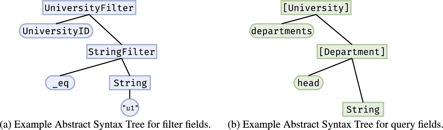
In general, a GraphQL query can be represented using a single AST that contains nodes representing the fields requested in the query, and also contains additional nodes for the input arguments that may be used for each of these fields. In our approach, we assume that each query accepts an input argument which captures the notion of a filter condition. Therefore, we specify the query evaluation in two steps: (i) evaluating for a filter condition, which is represented via an input argument that is defined as an input object type in the schema, (ii) evaluating for those fields that are requested in the GraphQL query. For instance, in the query example shown in Listing 3, the field having a filtering condition is different from the requested fields (the former is UniversityID while the latter includes departments and head). In the evaluation step for the filter condition, the identifier information of the filtered out instances of the requested type (i.e., University) are obtained after accessing the underlying data sources. In the next step, the underlying data sources are accessed again to retrieve only the requested fields for the filtered instances. Therefore, to enable such two steps in the query evaluation, we use multiple ASTs to represent a GraphQL query (cf. Fig. 3, these two ASTs represent the query shown in Listing 3), one of which captures the input argument structure (Fig. 3a), and the other of which captures the structure of the query, including the requested fields and their types (Fig. 3b). More specifically, every node in such ASTs represents either a named type (i.e., object type, interface type, input type, or scalar type), a wrapping type, or a field. Additionally, ASTs that represent input arguments also contain nodes that represent the values of scalar-typed fields (e.g., “u1” in the AST shown in Fig. 3a). The types (i.e., UniversityFilter, StringFilter, String) or wrapping types (i.e., [University], [Department]) are drawn with rectangle nodes. The fields (i.e., UniversityID, _eq, departments, head) are drawn with rounded rectangle nodes.
In practice, a filter condition is converted into disjunctive normal form (DNF).77 A query result in DNF contains data formed by the union of data that satisfies each disjunct. Therefore, in the step of evaluating for a filter condition: (i) multiple ASTs are generated where each represents one of the disjuncts, (ii) the underlying data source are accessed several times to obtain instances satisfying each disjunct, (iii) a union of identifier information for these instances of the requested type is returned.
5.2.RDF Mapping Language (RML)
Listing 8.
Example of RML mappings transforming university domain data, defined based on the example ontology as shown in Fig. 1
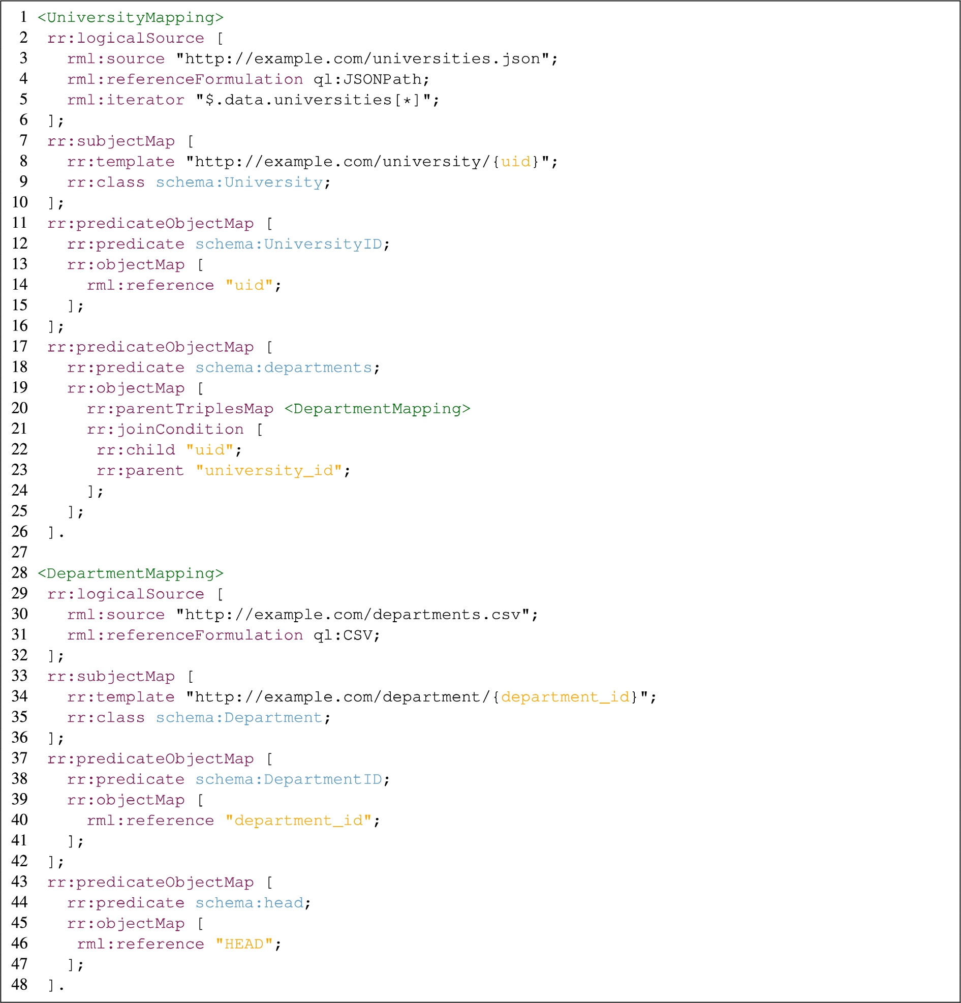
RML is a declarative mapping language for linking data to ontologies [51]. An RML document has one or more Triples Maps, which declare how input data is mapped into triples of the form (subject, predicate, object). An example of RML mappings is shown in Listing 8. A Triples Map contains the following three components (Logical Source, Subject Map and a set of Predicate-Object Maps). A logical source declares the source of input data to be mapped. It contains definitions of source that locate the input data source, reference formulation declaring how to refer to the input data, and logical iterator declaring the iteration loop used to map the input data. For instance, line 2 to line 6 in Listing 8 constitute the definition of a logical source. The definition declares that the data source is a JSON-formatted data source on the Web and also describes the way of iterating the JSON-formatted data (line 5). A subject map declares a rule for generating subjects when transforming underlying data into triples, including how to construct URIs of subjects (e.g., line 8) and specifying the concept to which subjects belong (e.g., line 9). A predicate-object map consists of one or more predicate maps declaring how to generate predicates of triples (e.g., line 12), and one or more object maps or referencing object maps defining how to generate objects of triples. An object map can be a reference-valued term map or a constant-valued term map. The former declares a valid reference to a column (relational data sources), or to an object (JSON data sources). The latter declares the value of the object as constant data. For instance, line 39 to line 41 make up a reference-valued term map. Line 19 to line 25 constitute a definition of a referencing object map including the join condition based on two triples maps. A referencing object map refers to another triples map (called a parent triples map) by using a rr:joinCondition property to state the join condition between the current triples map and the parent triples map. A join condition contains two properties, rr:child and rr:parent, of which the values must be logical references to logical sources of the current triples map and the parent triples map, respectively.
5.3.Components of the generic resolver function
Fig. 4.
Technical components in the generic resolver function.
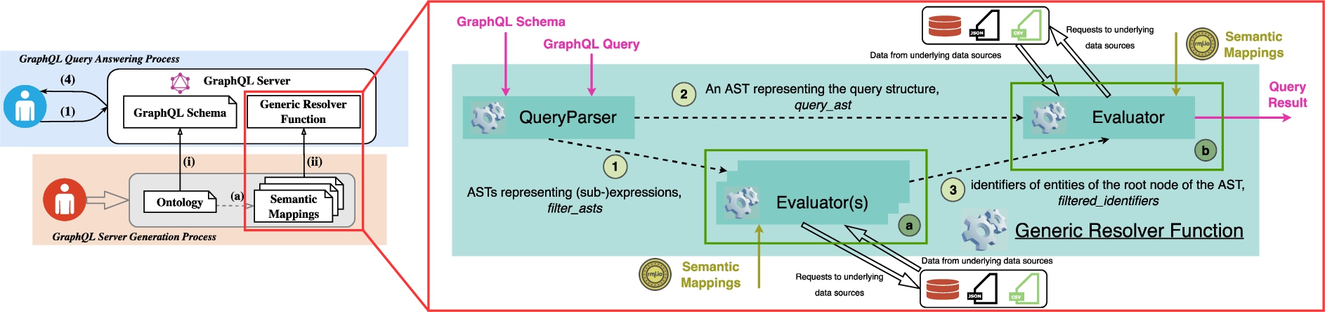
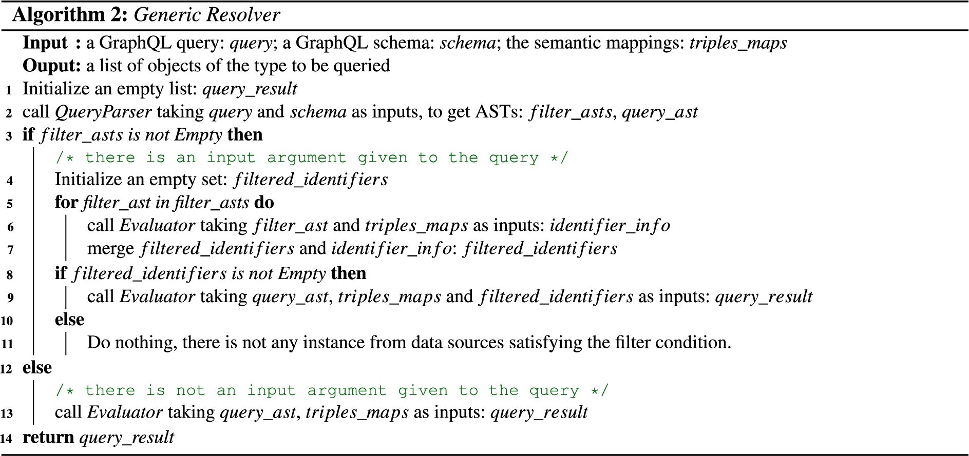
We show the basic technical components of the generic resolver function including QueryParser and Evaluator in Fig. 4. In Algorithm 2, we show the generic resolver function. The inputs to the generic resolver function are a GraphQL schema, a GraphQL query and semantic mappings. The GraphQL query and schema are inputs of the QueryParser. The QueryParser parses a query including a filter expression given as an input argument, and outputs the corresponding ASTs (Fig. 3) for the input argument and the query structure, respectively (shown as arrows 1◯ and 2◯ in Fig. 4). As mentioned in Section 5.1, in our practical solution a filter condition is converted into disjunctive normal form. In Algorithm 2, the QueryParser parses the query, converts a filter expression into a union of conjunctive expressions, and generates an AST for each conjunctive expression and an AST for the query structure (line 2). Then, the filter expression (line 5 to line 7 in Algorithm 2, frame a◯ in Fig. 4) and the query fields (line 9 and line 13 in Algorithm 2, frame b◯ in Fig. 4) are evaluated. The Evaluator is responsible for sending requests to underlying data sources and fetching data according to an AST. During evaluation of the filter expression, for each AST representing a conjunctive (sub-)expression, an evaluator is called to request data that satisfies the conjunctive (sub-)expression (line 6). After a call to an evaluator based on an AST (filter_ast in line 6), data representing the requested type, which contains identifier information, is returned (identifier_info in line 6). Taking the query in Listing 3 represented by the ASTs shown in Fig. 3 as an example, the requested type is University and data that can identify university instances is supposed to be returned in identifier_info. Such identifier information is captured in semantic mappings, which are used to construct the URIs for subjects where such subjects represent instances of the University concept. For instance, in line 8 of the RML mappings example in Listing 8, the values of the uid attribute of the underlying data source are used to construct URIs of subjects representing instances of the University concept. The identifier information returned by evaluating each filter_ast is merged into filtered_identifiers (line 7). During evaluation of the query fields, such merged identifier information is taken into account in the call to the evaluator of the query fields (line 9 in Algorithm 2, arrow 3◯ in Fig. 4).
As mentioned in Section 4.3, by generating the GraphQL schema based on an ontology, we can therefore, for each object or interface type and each field declaration, find the corresponding concept and relationship in the ontology. Since such concepts and relationships are used to define semantic mappings, when a generic resolver function retrieves data from the underlying sources of a requested type and relevant fields, it can therefore understand the semantic mappings regarding how to access underlying data sources and structure the returned data according to the GraphQL schema. Taking the query in Listing 3 represented by the ASTs shown in Fig. 3 as an example, as the requested type is University, the generic resolver function can therefore make use of relevant triples maps (line 1 to line 26 in Listing 8) defined in semantic mappings which are used for transforming underlying data following the semantics related to the University concept in the ontology.
5.4.The Evaluator algorithm
Algorithm 3:
Evaluator
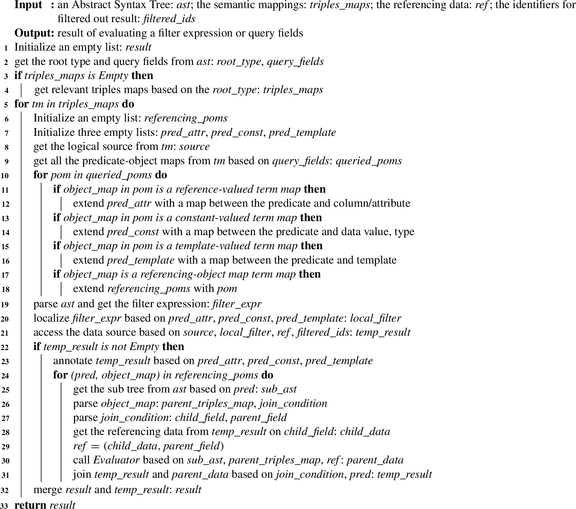
We present the details of Evaluator in Algorithm 3 and show an example in Fig. 5 of how evaluators work for answering the query in Listing 3. An AST and a number of triples maps from the semantic mappings are essential inputs to the algorithm. For a given AST, we can obtain the object type and fields that are requested in the query based on the root node and child nodes, respectively (line 2). For instance, taking the ASTs in Fig. 3 as examples, the root type and the field for evaluating the filter expression are University and UniversityID, and the root type and the first level requested field for evaluating query fields are University and departments, respectively. After getting the relevant triples maps based on the root node type (line 3 in Algorithm 3, e.g., UniversityMapping in Listing 8) or from the argument (line 16, the parent triples map, DepartmentMapping, which is an argument in the recursive call of an evaluator), the algorithm iterates over triples maps and merges the data obtained based on each triples map (line 4 to line 17). Exploring this in more detail, the algorithm parses each triples map to get the logical source and relevant predicate-object maps (line 5 and line 5). As described in Section 5.2, there are three different types of predicate-object map depending on the different maps of object, which are a reference-valued term map, a constant-valued term map or a referencing-object map. The algorithm iterates over the predicate-object maps and parses each one (line 5 to line 13). For a reference-valued term map, the mapping between the predicate and the reference column or attribute is stored (line 7, e.g., {UniversityID: uid} is stored in pred_attr), which will be used for rewriting a filter expression according to the underlying data source (line 14, e.g., uid = ‘u1’), annotating the obtained underlying data (line 15, e.g., HEAD is annotated as head for Department data). For a constant-valued term map, the mapping between the predicate and the constant data value, type is stored (line 9). For a template-valued term map, the mapping between the predicate and the template format is stored (line 11). All the
Fig. 5.
Example for answering the query in Listing 3, (1)–(3) indicate the requests to and responses from the data sources; (a)–(c) indicate the parameter passing between the calls to evaluators; (4) indicates a recursive call to evaluator for getting the data of departments; frame (A) indicates a join operation.
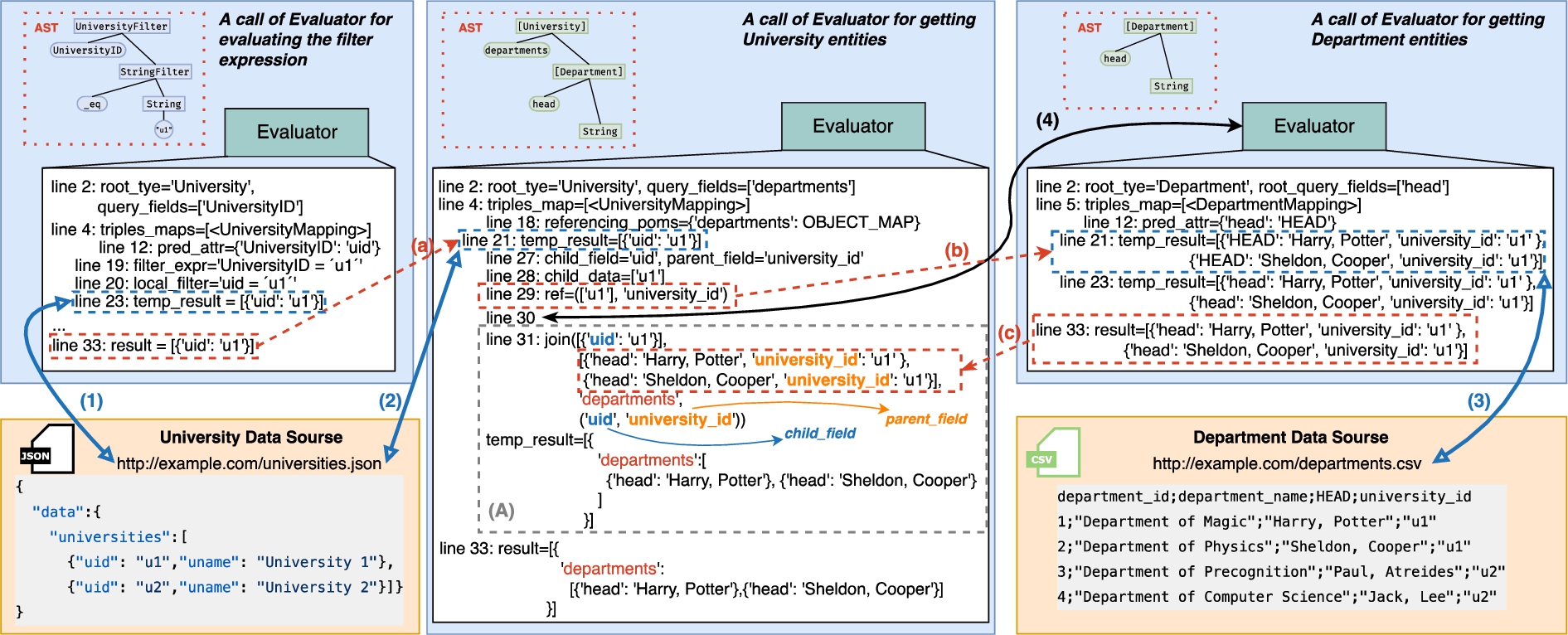
In the phase of evaluating a filter expression, local_filter, which represents the rewritten filter expression, is a necessary argument when sending requests to underlying data sources (line 14). While in the phase of evaluating query fields, filter_ids, being a NULL value or having at least one element, is a necessary argument (line 14, arrow (a) in Fig. 5). A NULL value represents the fact that the GraphQL query does not include an input argument. After obtaining the data from the underlying data sources, the data is serialized into JSON format (key/value pairs) in which the keys are predicates stated in the predicate-object map (line 15), where each predicate corresponds to a field in the GraphQL schema. In the next step, the algorithm iterates over predicate-object maps in which the object map refers to another triples map (called a parent triples map) (line 15 to line 16). An evaluator is called again to fetch data based on this parent triples map (line 16, arrow (4) in Fig. 5). For the query example, the parent triples map refers to the DepartmentMapping. Since such a referencing-object map definition states the join condition between the current triples map (UniversityMapping) based on
6.Related work
The widely used Semantic Web-based techniques and the recently developed GraphQL have led to a number of works relevant to our GraphQL-based framework for data access and data integration. We extend the summary of approaches presented in [17] by adding several new related approaches and new perspectives on the comparison. Table 2 summarizes these systems and our approach. These systems can be divided into two categories, namely OBDA-based systems and GraphQL-based systems. The former group contains Morph-RDB [49,52], Morph-CSV [19], Ontop [13,50], Squerall [47] and Ontario [28]. The latter group consists of GraphQL-LD [60], HyperGraphQL [55], UltraGraphQL [32,56], Morph-GraphQL [17], Ontology2GraphQL [30] and our OBG-gen. OBG-gen can also be categorized as an OBDA-based system in the first group. In addition to the two groups described above, there is another system that is related to our work. It is OBA [31], which is an ontology-based framework that facilitates the development of REST APIs for knowledge graphs.
Table 2
Summary of related approaches
| Approach | Service setup (preparation) process | Query answering process | |||
| Input | Output | Input | Output | Underlying data | |
| Morph-RDB [49,52] | Semantic mappings | – | SPARQL query | SQL query | Relational data |
| Morph-CSV [19] | Semantic mappings, tabular metadata | – | SPARQL query | SQL query | Tabular data |
| Ontop [13,50] | Semantic mappings | – | SPARQL query | Queries based on data sources | Relational data, non-relational data via database federators |
| Squerall [47] | Semantic mappings | – | SPARQL query | Queries based on data sources and their wrappers | Diverse data sources in a Data Lake |
| Ontario [28] | Semantic mappings | – | SPARQL query | Queries based on data sources and their wrappers | Diverse data sources in a Data Lake |
| GraphQL-LD [60] | – | – | GraphQL query, JSON-LD context | SPARQL query | SPARQL endpoint |
| HyperGraphQL [55] | – | GraphQL server (manually) | GraphQL query, JSON-LD context | SPARQL query | SPARQL endpoint |
| UltraGraphQL [32,56] | RDF schemas of SPARQL endpoints | GraphQL server (automatically) | GraphQL query, JSON-LD context | SPARQL query | SPARQL endpoint |
| Morph-GraphQL [17] | Semantic mappings | GraphQL server (automatically) | GraphQL query | SQL Query | Relational data |
| Ontology2GraphQL [30] | A meta model, an ontology follows the model | GraphQL server (automatically) | GraphQL query | SPARQL query | SPARQL endpoint |
| OBA [31] | An ontology | Open API specification, a REST API server (automatically) | API requests | SPARQL query | SPARQL endpoint |
| OBG-gen | Semantic mappings, an ontology | GraphQL server (automatically) | GraphQL query | SQL query, API requests | Relational data, tabular data, JSON-formatted data |
As a new perspective to the summary in [17], all the approaches (except for GraphQL-LD) have two processes: (i) the service setup (preparation) process and (ii) the query answering process. During the service setup process, all OBDA-based approaches need semantic mappings as input. In these systems, semantic mappings are used in a similar manner to represent differences between global and local schemas, namely mapping translations as highlighted in [21]. Some approaches take additional resources as inputs. Morph-CSV uses CSVW88 to annotate tabular data. OBG-gen needs an ontology and semantic mappings together in order to generate a GraphQL server that is intended not only for semantics-aware data access but for data integration.99 Another system that also uses ontologies in the service setup process is OBA. OBA generates an OpenAPI Specification (OAS)1010 based on ontologies. It is also highlighted in [21] that the diversity of how underlying data sources provide data brings challenges to mapping translations. For instance, REST is a popular architecture for web services and is commonly used for Web-based applications to provide data since 2000. GraphQL becomes an alternative since 2012. In this respect, OBA, OBG-gen and Morph-GraphQL explore how semantic resources (i.e., ontologies and semantic mappings) can be used to provide access to data that is provided by Web APIs. For the other GraphQL related work, Ontology2GraphQL needs a meta model for the GraphQL query language and requires an ontology following the meta model for generating the GraphQL schema. HyperGraphQL requires no inputs during the service setup process, but the developer must build the GraphQL server from scratch. UltraGraphQL, based on HyperGraphQL, requires RDF schemas of SPARQL endpoints for bootstrapping the GraphQL server. In actuality, GraphQL-LD does not require any GraphQL servers, but instead focuses on how to represent GraphQL queries using SPARQL algebra and how to convert the results of a SPARQL query into a tree structure in response to a GraphQL query.
For the query answering process, OBDA-based approaches (i.e., Morph-RDB, Morph-CSV, Ontop, Squerall and Ontario) accept SPARQL queries and translate them into specific queries. Morph-RDB handle underlying data stored in relational databases, while Morph-CSV deals with data stored in CSV files. Morph-RDB and Morph-CSV translate SPARQL queries into SQL queries. Ontario, Squerall and Ontop support heterogeneous data sources. These three systems can translate SPARQL queries into various queries according to the query languages of the underlying data sources or queries accepted by data source wrappers. Our approach, OBG-gen, accepts relational data, tabular data and JSON-formatted data as the underlying data. Moreover, OBG-gen can integrate data in different formats from multiple sources, due to the generic resolver function implementation that can structure obtained data in the JSON format according to the GraphQL schema. The remaining approaches are based on underlying data in SPARQL endpoints and translate GraphQL queries into SPARQL queries (GraphQL queries for GraphQL-based approaches, API requests for OBA). GraphQL-LD, HyperGraphQL, and UltraGraphQL require context information expressed in JSON-LD. Such JSON-LD context information contains URIs of classes to which instances in the RDF data belong.
In addition, we study relevant OBDA/OBDI and GraphQL benchmarks to conduct our experiments and evaluation. These benchmarks are Berlin SPARQL Benchmark (BSBM) [12], Norwegian Petroleum Directorate Benchmark (NPD) [42], GTFS-Madrid-Bench [18], ForBackBench [2] and Linköping GraphQL Benchmark (LinGBM) [20]. These OBDA/OBDI related benchmarks are built based on different use cases (BSBM for the e-commerce use case, NPD for the oil industry, GTFS-Madrid-Bench for the transport domain, ForBackBench reusing data from other benchmarks) and focus on testing different abilities of OBDA/OBDI engines. In more detail, the BSBM benchmark aims to test and compare the performance of native RDF stores with engines implementing SPARQL-to-SQL query translation. The NPD benchmark can be used to analyze OBDA system implementations in terms of query rewriting, query unfolding and query execution. The GTFS-Madrid-Bench aims to test engines focusing on virtualized access to heterogeneous data. The above three benchmarks commonly focus on testing engines that contain query rewriting mechanisms, which are usually implemented by OBDA/OBDI engines. The ForBackBench benchmark has a focus on both data integration scenarios and data exchange scenarios. In the former scenarios, engines usually implement query rewriting mechanisms. While in the latter scenarios, engines usually implement forward-chaining algorithms (e.g., [16,48]) to populate a centralized data warehouse. Therefore, in contrast to the previous three benchmarks, ForBackBench focuses on comparing and analyzing systems across both two different mechanisms (i.e., query writing and forward-chaining algorithms). In terms of GraphQL-related benchmarks, the LinGBM benchmark is the first one that can be used to study the behavior of GraphQL server implementations at scale [20]. It provides a scalable dataset regarding the University domain and specifies key technical challenges (e.g., relationship traversal) of GraphQL server implementations. For the evaluation of our work (see next section), among these OBDA/OBDI and GraphQL related benchmarks, we choose GTFS-Madrid-Bench and LinGBM, respectively. The reasons are: (i) for the real case evaluation in the materials design domain, LinGBM can guide us to characteristic the GraphQL queries to better compare and analyze the abilities of GraphQL systems; (ii) by following the scenarios in LinGBM and GTFS-Madrid-Bench, we can test the ability of our approach to work for general different domains.
7.Evaluation
In this section, we present an evaluation of the framework shown in Section 3. We consider a real case application scenario in the materials design domain, and two synthetic benchmark scenarios based on the Linköping GraphQL Benchmark (LinGBM)1111 [20] and GTFS-Madrid-Bench1212 [18], respectively. The main goals of the evaluation are: (i) to validate that GraphQL can be used to assemble an integrated view of underlying data and manage requests to underlying data sources in an ontology-driven data access and integration scenario; (ii) to validate that the approach can work in general domains for data access and integration. Meanwhile, we intend to provide initial insights into the query performance of our approach by comparing it with existing OBDA-based and GraphQL-based solutions for data access and data integration. Therefore, the evaluation focuses on validating the generability and feasibility of our approach, and aims to answer the following detailed research questions:
RQ1: Can the generated GraphQL server provide integrated access to heterogeneous data sources? For instance in the real case application scenario, data from different sources may follow different models and is shared or queried in different ways.
RQ2: How does the generated GraphQL server compare to other OBDA-based systems and other GraphQL-based systems in terms of query performance and its behavior for increasing dataset sizes?
RQ3: Is the proposed approach, ontology-based GraphQL server generation, a general approach that can work in different domains for data access and integration?
In the first evaluation scenario based on the real case application scenario in the materials design domain, we aim to answer RQ1 and RQ2. In the second and third evaluation scenarios based on the LinGBM and the GTFS-Madrid-Bench benchmarks, we aim to answer RQ3 to validate the generability and feasibility of our approach. We performed all experiments on a server machine with Intel Xeon Gold 6130 @ 2.10 GHz CPUs. The machine runs a 64-bit CentOS Linux 7 (Core) operating system. We reserved 8 CPU cores and 4 GB memory for the experiments.
7.1.Real case evaluation
In the real case evaluation, we focus on a use case in the materials design domain where the task is data integration over two data sources, Materials Project [37] and OQMD (The Open Quantum Materials Database) [54].
Fig. 6.
Example of searching materials from materials project, OQMD and NOMAD.
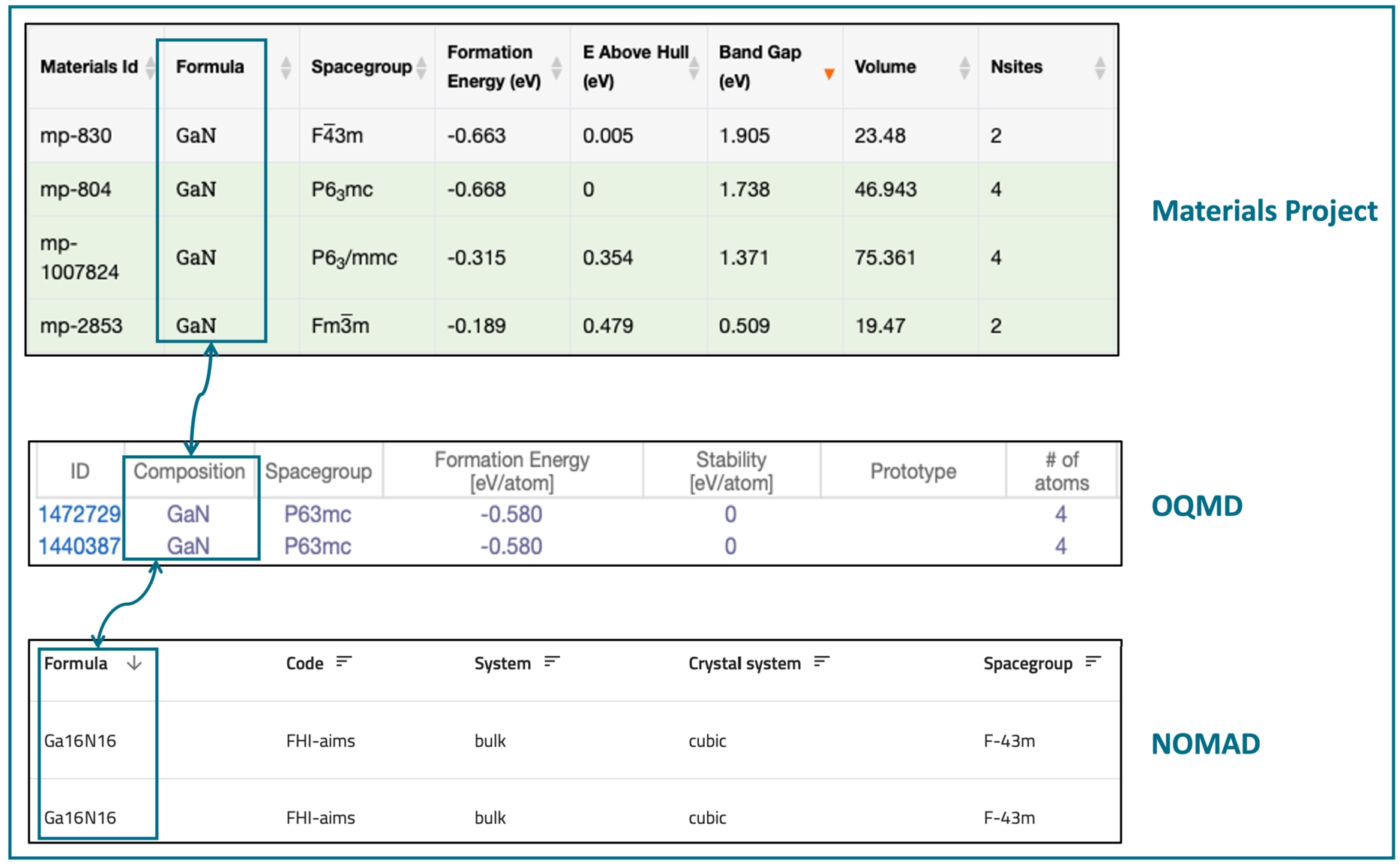
Motivation The materials science domain, like many other domains, is at an early stage when it comes to introducing Semantic Web-based technologies into its data-driven workflows. A large number of research groups and communities have thus developed a variety of data-driven workflows, including data repositories [40,41] and data analytics tools. As data-driven techniques become more prevalent, more data is produced by computer programs and is available from various sources, which leads to challenges associated with reproducing, sharing, exchanging, and integrating data among these sources [1,38,39,53,61]. Figure 6 illustrates an example of searching for gallium nitride materials with the reduced chemical formula of
Data We collect data from the Materials Project and OQMD representing five different types of real-world entities (Calculation, Structure, Composition, Band Gap and Formation Energy). We define semantic mappings (for all the systems, see the next paragraph) based on MDO to interpret such data. We collect data in the sizes of 1K, 2K, 4K, 8K, 16K and 32K from each database for populating the five entities. The size 1K means 1000 entities of each entity type. We represent this data in different formats such as tabular data for relational databases and for CSV files, and JSON-formatted data for JSON files. Additionally, for HyperGraphQL and UltraGraphQL in our evaluation, we create an RDF file based on RML mappings and MDO for each dataset setting. We have six dataset settings for the experiments, which are 1K–1K, 2K–2K, 4K–4K, 8K–8K, 16K–16K and 32K–32K. Taking 2K–2K as an example, for each entity type, the test data contains data in the size of 2K from Materials Project and 2K from OQMD, respectively.
Fig. 7.
Outline of the real case evaluation.
Systems We compare our tool, OBG-gen in two versions (OBG-gen-rdb and OBG-gen-mix) with four systems: Morph-RDB [49], Ontop [50], HyperGraphQL [55], and UltraGraphQL [56]. OBG-gen-rdb represents the case where the generated GraphQL server handles data in relational databases, and OBG-gen-mix represents the case where the generated GraphQL server handles data not only in relational databases but also data in JSON and CSV formats. They take different RML mappings as inputs. Morph-RDB and Ontop are representatives from the group of OBDA-based tools. They can access relational databases as data sources by translating SPARQL queries into SQL queries based on semantic mappings, written in R2RML. As for the group of GraphQL-related tools, we intended to include Morph-GraphQL and Ontology2GraphQL in our evaluation. However, Morph-GraphQL fails to parse mappings; Ontology2GraphQL cannot be run due to a lack of detailed instructions regarding its setup. In the case of GraphQL-LD, since it focuses on querying Linked Data via GraphQL queries and a JSON-LD context using a SPARQL engine instead of a GraphQL interface, we did not consider it in our evaluation. Therefore, HyperGraphQL and its extension UltraGraphQL are the GraphQL engines that are included in our evaluation. They can query Linked Data that may be provided by local RDF files and remote SPARQL endpoints. The semantic mappings for all the systems in the evaluation are based on MDO. OBG-gen generates the GraphQL schema based on MDO. UltraGraphQL and HyperGraphQL use a modified version of the generated schema since they require directive definitions to specify the correspondences between query entries and the data. Figure 7 shows how the systems are configured in the evaluation. HyperGraphQL and UltraGraphQL are provided with the same RDF data for each dataset setting. OBG-gen-rdb is provided with two MySQL database instances hosting data from the Materials Project and OQMD respectively. Morph-RDB and Ontop are provided with one single MySQL database instance hosting data from the two sources. Conceptually, OBG-gen-mix is also provided with two database instances. However, each instance contains different formats of data such as data in a MySQL database, or in CSV or JSON files. More detailed, the instance for Materials Project has Composition data in JSON format and Band Gap data in CSV format. The instance for OQMD has Structure and Band Gap data in JSON format and Formation Energy data in CSV format. The data representing other entities for each instance is stored in MySQL database instances.
Table 3
Features of queries without filter conditions
| Query | Choke points | Domain Interest (DI) | Result Size (RS) |
| Q1 | 2.1, 2.2 | L | |
| Q2 | 2.1, 2.2 | ✓ | L |
| Q3 | 1.1, 2.1, 2.2 | ✓ | L |
| Q4 | 1.1, 2.1, 2.2 | ✓ | L |
| Q5 | 2.2 | L |
Table 4
Features of queries with filter conditions
| Query | Choke points | Domain Interest (DI) | Diffs | Filter expression form | Result Size (RS) |
| Q6 | 1.1, 2.1, 2.2, 4.1, 4.4 | ✓ | A | C | |
| Q7 | 1.1, 2.1, 2.2, 4.1, 4.4 | ✓ | A & B | C | |
| Q8 | 1.1, 2.1, 2.2, 4.1, 4.4, 4.5 | ✓ | ✓ | A & (B | C) | C |
| Q9 | 1.1, 2.1, 2.2, 4.1, 4.4, 4.5 | ✓ | ✓ | A & B | C |
| Q10 | 1.1, 2.1, 2.2, 4.1, 4.4, 4.5 | ✓ | ✓ | A & (B & C) | NL |
| Q11 | 2.2, 4.1, 4.4, 4.5 | ✓ | (A & B) & ((A & B) | C) | NL | |
| Q12 | 2.2, 4.1, 4.4 | ✓ | A | NL |
Queries We create queries that cover different features, aiming to evaluate our system based on qualitative aspects regarding what functionalities the system can satisfy and quantitative aspects regarding how the system performs over different data sizes. Additionally, we use competency questions stated in the requirements analysis of MDO to create queries with domain interests. The features of queries without and with filter expressions are shown in Table 3 and Table 4, respectively. From the perspective of GraphQL, we consider which choke point a query covers. The details of choke points are introduced in LinGBM.1313 These choke points are regarding the key technical challenges. We characterize all queries using the perspectives of choke points, domain interest (DI), and result size (RS). DI indicates that the query is a domain-interest query. Such a query corresponds to a relevant competency question stated in the requirements analysis of MDO. For RS, as the dataset grows, we consider whether the result size increases linearly (L) or more than linearly (NL), or stays a constant value (C). For queries with filter expressions we take into account the filter expression form and whether the filtering AST differs from the query AST (Diffs), such as in the example in Fig. 3b where the filtering AST and the query AST are different.
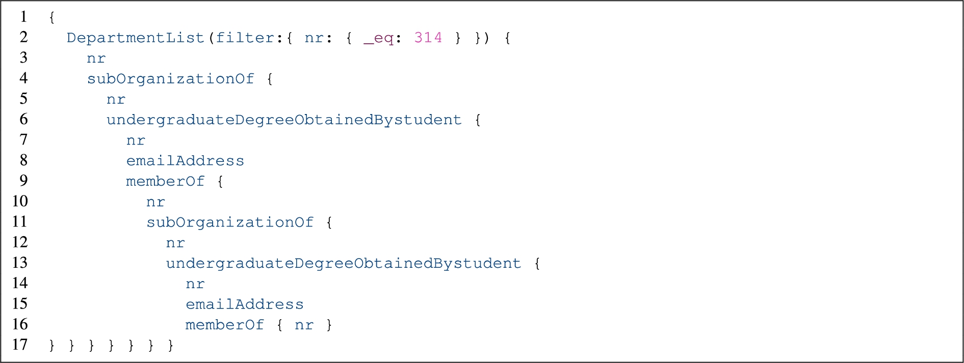
Table 5 shows more details of meanings of different filter expressions for Q6–Q12. The filter expressions for Q6 and Q12 are simpler than those for Q7–Q11 where the filter expressions have sub-expressions connected by boolean operators. Query features in terms of DI, and the filter expression form can help us understand systems qualitatively; Diffs and RS help in understanding systems quantitatively in the scaling analysis over different data sizes. We show Q1 in Listing 10 and Q7 in Listing 12. The results of these two queries are given in Listing 11 and Listing 13, respectively. Q1 requests all the structures containing the reduced chemical formula of each structure composition. Q7 requests all the calculations where the ID is in a given list of values, and the reduced chemical formula is in a given list of values.
Table 5
Meanings of filter expressions in Q6 to Q12
| Query | Filter expression meaning |
| Q6: A | Id is in a list |
| Q7: A & B | Id is in a list and reduced chemical formula is in a list |
| Q8: A & (B | C) | Id is in a list and (reduced chemical formula is in list |
| Q9: A & B | Property name is “Band Gap” and value is greater than 5 |
| Q10: A & (B & C) | Reduced chemical formula is in a list and (property name is “Band Gap” and value is greater than 5) |
| Q11: (A & B) & ((A & B) | C) | (Property name is “Band Gap” and value is greater than 4) and ((property name is “Band Gap” and value is greater than 4) or reduced chemical formula is in a list) |
| Q12: A | Reduced chemical formula contains silicon element |
Experiments and measurements We evaluate the query execution time (QET) of the different systems over the six dataset settings. Separately for each query, we run the query four times and always consider the first run to be a warm-up, then take the averaged value of the remaining three runs. Figure 8 illustrates the measurements over the six data sizes per query (Q1–Q12). Figure 9 and Figure 10 illustrate the measurements of all systems per data size for queries without filtering conditions and with filtering conditions, respectively. The measures for all data sizes and all queries are available online.1414 For UltraGraphQL, we have measurements only for queries Q1–Q4 because UltraGraphQL does not support queries with filtering conditions. For HyperGraphQL answering queries with filter expressions, we have only the measurement for Q6 because the system can only deal with filtering by resource IRIs.
Fig. 8.
Query Execution Time (QET) per query on materials dataset.
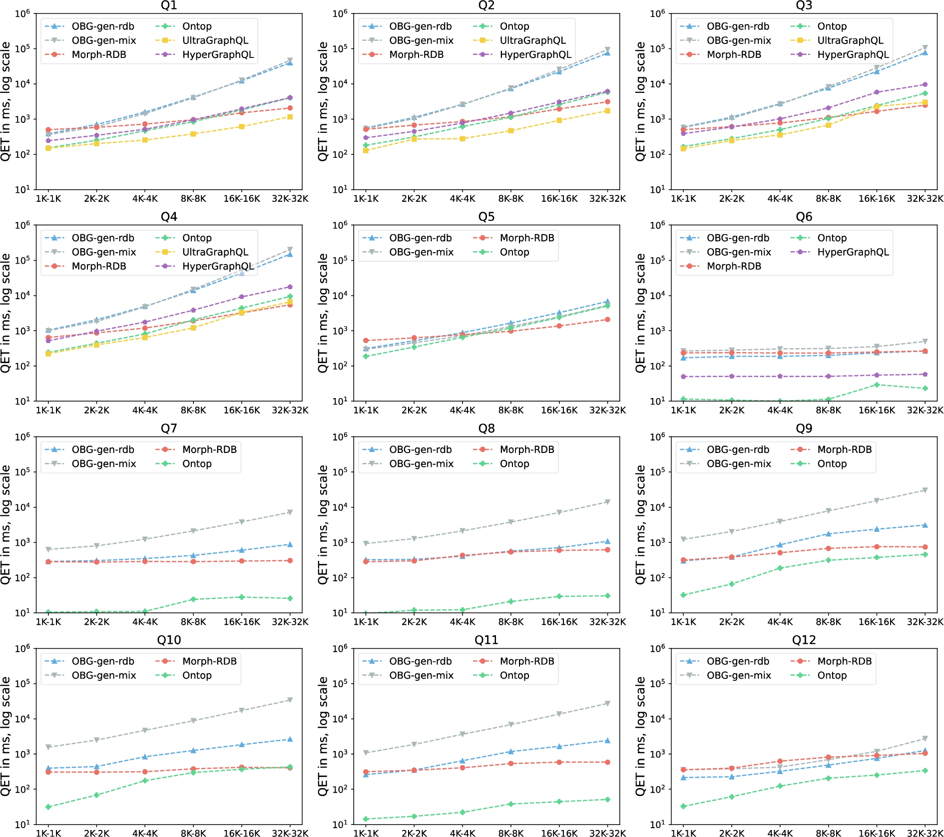
Results and discussion By analyzing the obtained measurements, we summarize three observations. The first observation is that both GraphQL servers generated by OBG-gen-rdb and OBG-gen-mix can answer all 12 of the queries covering different features (such as choke points). Therefore, the framework presented in Section 3 is feasible for data access and integration; this answers RQ1. Particularly, the GraphQL schema generated based on the ontology can provide an (integrated) view of underlying (heterogeneous) data; the generic resolver function based on the semantic mappings is capable of accessing heterogeneous data sources, combining the retrieved data (which may be in different formats), and structuring the data according to the GraphQL schema.
The second observation is regarding queries without filtering conditions (Q1–Q5) (cf. Figs 8 and 9). All of the systems have increases of QETs as the size of the dataset increases. However, Morph-RDB is less sensitive to the data size increase compared with other systems. UltraGraphQL and HyperGraphQL outperform other systems for some smaller datasets (e.g., UltraGraphQL’s QETs of Q1 and Q2, HyperGraphQL’s QETs for Q1 from 1K–1K to 4K–4K). We explain this by the fact that these two systems have additional context information declaring URIs of classes to which instances in the RDF data belong, which is unlike the other systems which have to make use of semantic mappings to output queries to be evaluated against the underlying data sources. OBG-gen-rdb outperforms Morph-RDB for some queries in smaller datasets (e.g., Q1 in 1K–1K, Q5 in 1K–1K and 2K–2K). For some queries, OBG-gen-rdb and Morph-RDB have close QETs (e.g., Q2 in 1K–1K). Ontop outperforms the other two in smaller datasets (e.g., Q1 in 1K–1K to 8K–8K, Q5 in 1K–1K to 4K–4K), but is more sensitive to data size increase compared with Morph-RDB.
Fig. 9.
Query Execution Time (QET) per data size on materials dataset for queries without filtering conditions.
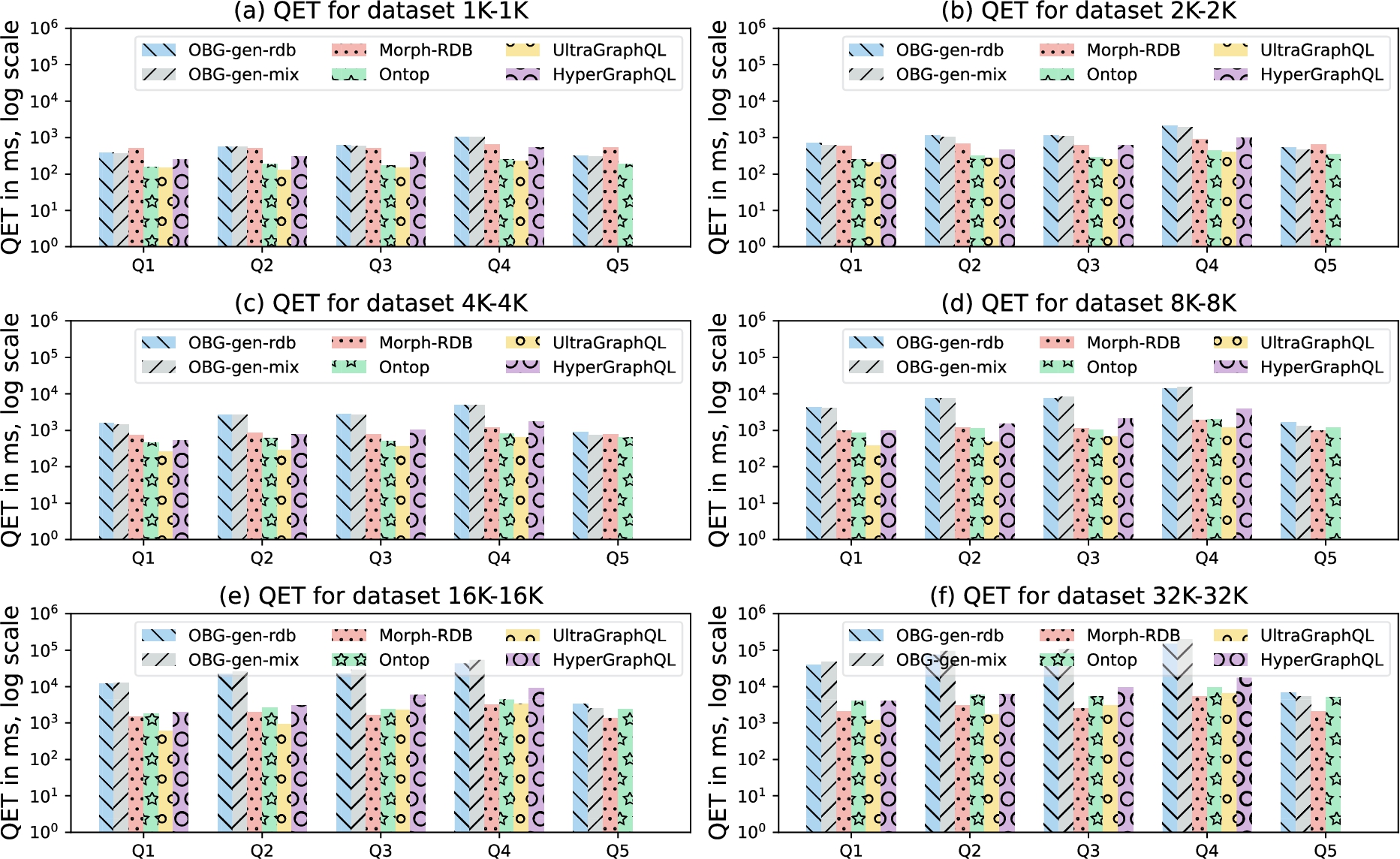
Fig. 10.
Query Execution Time (QET) per data size on materials dataset for queries with filtering conditions.
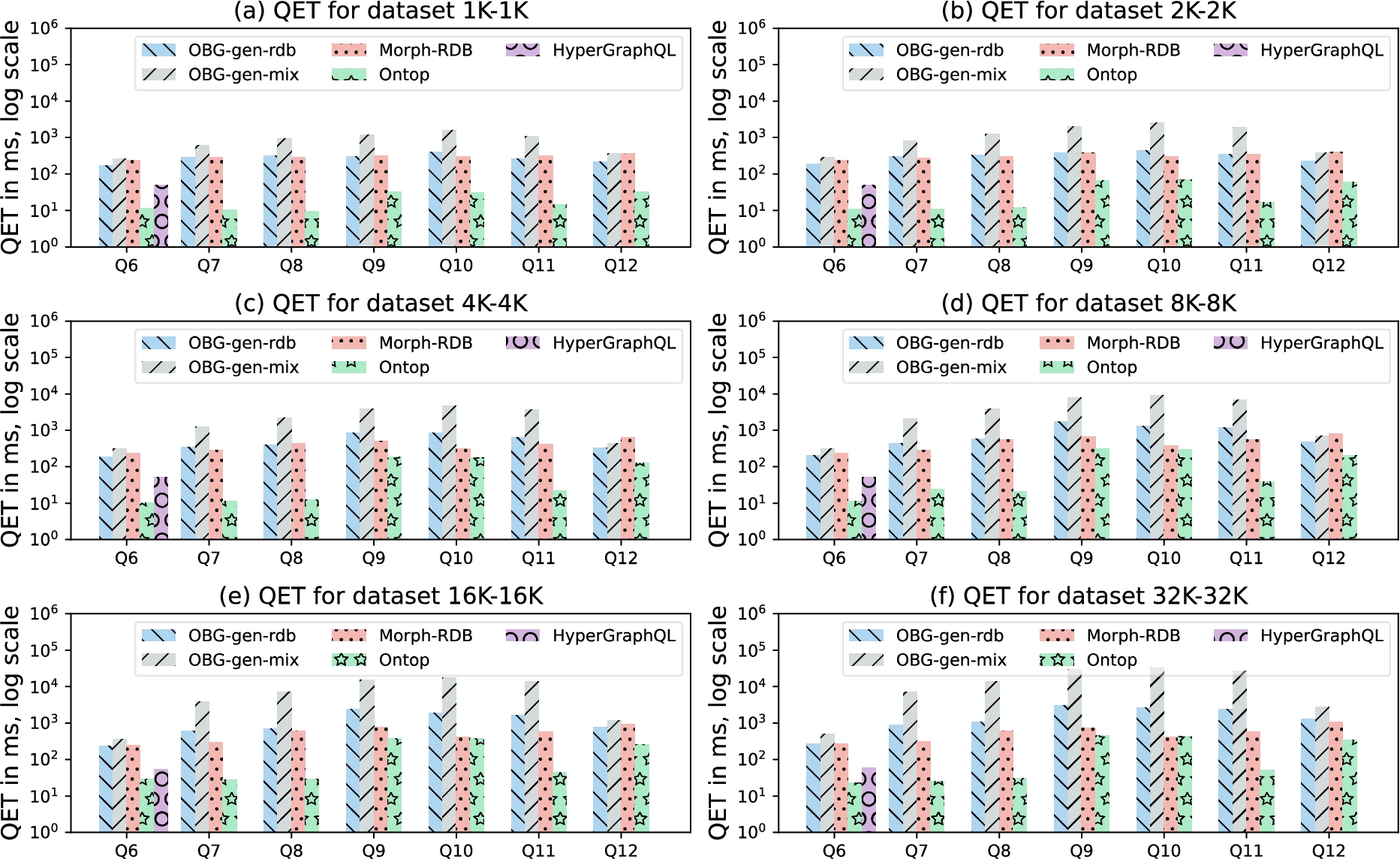
The third observation is regarding how OBG-gen-rdb, Ontop and Morph-RDB perform for queries with filter conditions (Q6–Q12) (cf. Figs 8 and 10). Ontop outperforms the other two engines in most cases but is more sensitive to increases in dataset size (e.g., Q9 from 1K–1K to 8K–8K). According to [13], Ontop has a mapping optimization step which is not included in the query execution period. This could be a reason why Ontop outperforms the other engines. OBG-gen-rdb and Morph-RDB behave similarly for Q6 with stable QETs and Q12 with slight increases, as the data size increases. As Table 4 shows, the result size of Q6 is a constant over all the datasets in different sizes. Additionally, the filter expressions for Q6 and Q12 are simpler compared with those of Q7–Q11. Therefore, the QETs for evaluating filtering expressions for Q6 and Q12 are less than those of Q7–Q11. For other queries (Q7–Q11) Morph-RDB outperforms OBG-gen-rdb, however the differences between the two systems are less than those for queries without filtering conditions (e.g., Q1–Q4). The filtering conditions in GraphQL queries for OBG-gen-rdb and in SPARQL queries for Morph-RDB are written within WHERE clauses in SQL queries, thus will be evaluated against the back-end databases. A similar observation is also found in [17] where the experiment metrics shows that Morph-RDB outperforms other systems (e.g., Morph-GraphQL) as the size of dataset increase due to the SPARQL to SQL optimizations [17].
Based on the second and the third observations, we can answer the research question RQ2. The GraphQL servers generated by OBG-gen perform similarly compared with other systems for queries without filtering conditions, but are more sensitive to the increase of datasets even they can outperform for some queries in smaller datasets. By comparing OBG-gen-rdb, Ontop and Morph-RDB, we summarize the reasons as follows. As shown in Section 5, the implementation of OBG-gen is based on representing a GraphQL query with Abstract Syntax Trees (Fig. 3). In this way, two basic requests are sent to underlying data sources to get the data with respect to the semantic mappings. While for Morph-RDB and Ontop, based on semantic mappings, a SPARQL query is translated into a single SQL query. For queries with filtering conditions, all the three engines (OBG-gen-rdb, Morph-RDB and Ontop) can take the advantages of rewriting filter conditions into SQL queries so that the QETs do not show a significant increase as the data size increases.
7.2.Evaluation based on LinGBM (Linköping GraphQL Benchmark)
To show the generalizability of our system, we conduct an evaluation based on LinGBM. LinGBM provides tools for generating datasets (data generator)1515 and queries (query generator),1616 and for testing execution time and response time (test driver).1717
Data The dataset generated by the data generator is a scalable, synthetic dataset regarding the University domain, including several entity types (e.g., University and Department). We generate data in scale factors (
Listing 9.
A query according to QT5, such a query goes from a given department to its university, then retrieves all graduate students who get the bachelor’s degree from the university, then comes back to department. This cycle is repeated two times
Queries The experiments are performed over eight query sets, where each set contains 100 queries that are generated using the LinGBM query generator based on a query template (QT). A query template has placeholders for input arguments. The query generator can generate a set of actual queries (query instances) based on a query template in which the placeholder in the query template is replaced by an actual value. We select eight query templates (QT1–QT6, QT10 and QT11) for constructing eight query sets (QS1–QS8). We show an example query according to QT5 in Listing 9. The other six query templates from LinGBM require GraphQL servers to have implementations for functionalities such as ordering and paging which are not considered currently by OBG-gen. However, these functionalities are interesting for future extension of OBG-gen.
Experiments, results and discussion Same as the real case evaluation, we evaluate the query execution time (QET) of our system on the three datasets. Each query from a query set is evaluated once. We show the average query execution times for the different query sets in Table 6. Based on the obtained measurements, we observe that our system has slight increases for QS1, QS2, QS4, QS6 and QS7 in terms of the average QETs. For QS3, the average QET is stable for all the three datasets. For QT5, the increase from 0.51 seconds at data scale factor 20 to 13.85 seconds at data scale factor 100 is due to the dramatic increase in result size. More specifically, the queries in QS5 and QS8 need to access the ‘graduateStudent’ table which increases dramatically in size from 50,482 rows in the table (
Table 6
Average QET (in seconds) in the evaluation based on LinGBM
| Scale factor | QS1 (QT1) | QS2 (QT2) | QS3 (QT3) | QS4 (QT4) | QS5 (QT5) | QS6 (QT6) | QS7 (QT10) | QS8 (QT11) |
| 4 | 0.11 | 0.13 | 0.12 | 0.15 | 0.19 | 0.13 | 0.10 | 0.26 |
| 20 | 0.12 | 0.15 | 0.12 | 0.18 | 0.51 | 0.15 | 0.18 | 0.90 |
| 100 | 0.15 | 0.27 | 0.12 | 0.26 | 13.85 | 0.23 | 0.72 | 4.41 |
7.3.Evaluation based on GTFS-Madrid-Bench
We furthermore demonstrate the generalizability of our system by evaluating it against GTFS-Madrid-Bench, which is a benchmark for evaluating OBDI systems.
Data, queries and systems The dataset provided by GTFS-Madrid-Bench is a scalable dataset regarding the Transport domain (the metro system of Madrid), including several entity types (e.g., Route, Stop, Shape and Trip). We use the data generator provided by GTFS-Madrid-Bench to generate data in scale factors (
Experiments, results and discussion Same as the previous two evaluation scenarios, we evaluate the query execution time (QET) of systems on different datasets. We show the measurements in Table 7. According to the measurements, both OBG-gen-rdb and Ontop show increases in QETs for all four queries as the dataset increases. However, as with the observation in the real case evaluation, Ontop behaves less sensitively to the increase in dataset. In terms of how the two systems behave for different queries, both engines spend more time to answer Q1 (without any filter conditions) and Q9 (with several relationship retrievals). For answering Q1, OBG-gen-rdb spends more than 3,600 seconds for scale factors 10 and 50. Although Ontop is able to answer Q1 in less time than OBG-gen, it cannot finish the execution because it runs out of the reserved 4 GB memory for scale factor 50. More specifically, Q1 needs to access the ‘Shape’ table which increases dramatically in size from 58,540 rows in the table (
Table 7
QET (in seconds) in the evaluation based on GTFS-Madrid-Bench
| Scale factor | System | Q1 | Q2 | Q3 | Q4 | Q5 | Q9 | Q13 |
| 1 | OBG-gen-rdb | 82.220 | 0.373 | 0.337 | 0.085 | 0.093 | 209.441 | 0.425 |
| Ontop | 7.311 | 0.132 | 0.100 | 0.014 | 0.035 | 44.003 | 0.058 | |
| 5 | OBG-gen-rdb | 2610 | 1.743 | 1.413 | 0.115 | 0.153 | out of memory | 1.633 |
| Ontop | 37.596 | 0.480 | 0.384 | 0.030 | 0.094 | 252.040 | 0.128 | |
| 10 | OBG-gen-rdb | time out | 4.700 | 3.030 | 0.143 | 0.134 | time out | 4.048 |
| Ontop | 75.072 | 0.939 | 0.703 | 0.048 | 0.129 | out of memory | 0.235 | |
| 50 | OBG-gen-rdb | time out | 84.159 | 50.125 | 0.255 | 0.378 | time out | 48.683 |
| Ontop | out of memory | 8.052 | 4.044 | 0.155 | 0.340 | time out | 0.839 |
7.4.Summary
For evaluating our approach, ontology-based GraphQL server generation, we conducted an experiment motivated by the materials design domain and experiments based on two synthetic benchmark scenarios (LinGBM and GTFS-Madrid-Bench). Based on the measurements of these experiments, we can answer the three research questions presented at the beginning of Section 7. Our approach can generate GraphQL servers for data access and data integration and can be used in various domains (RQ1 and RQ3). The other GraphQL interfaces, HyperGraphQL and UltraGraphQL, can be used for data integration to a limited extent due to the fact that they do not support various filter conditions. This means questions with filter conditions cannot be answered. By comparing our approach with other well-known systems (RQ2), we learn that our system can perform relatively similar to others (e.g., Morph-RDB) in terms of QETs for queries with filter conditions (as shown in Fig. 10), and for some queries without filter conditions in smaller datasets (as shown in Fig. 9). Morph-RDB and Ontop are both less sensitive to the data size increase. The reason for this can be explained by the fact that they have optimization techniques that enable queries to be executed in a shorter amount of time. For instance, Ontop has a mapping optimization step which is not included in the query execution period [13,62]; Morph-RDB has a query rewriting optimization step where projections and selections are pushed down for removing non-correlated subqueries [52,62]. However, our approach supports data integration where the underlying data is from different kinds of sources (i.e., OBG-gen-mix), in contrast to Morph-RDB that only support data integration where the underlying data is from relational databases. This is due to the implementation of the generic resolver function presented in Section 5, that combines data from multiple sources according to a GraphQL schema, as an integrated view of underlying data. Moreover, OBG-gen-mix can integrate data where underlying data is provided in different ways. In contrast, the other systems require the underlying data to be materialized as RDF triple stores (e.g., UltraGraphQL and HyperGraphQL) or to be stored in one single database (e.g., Morph-RDB and Ontop).
8.Discussion and future work
We emphasize that our work aims to enable GraphQL for not only data access (as other GraphQL-based approaches) but also data integration, by automatically generating the server based on an ontology and semantic mappings. Our work presents the first solution to this problem. Essentially, our approach concentrates on providing data access and integration using an ontology in a GraphQL setting with an approach that provides support for practical applications. In this respect, our work fills a gap in GraphQL applications (e.g., [17,30,32,55,60]). Compared with existing GraphQL-based approaches (e.g., UltraGraphQL [32] and HyperGraphQL [55]) for data access, our approach provides more GraphQL query features by supporting arbitrary filtering conditions. Our work can also provide an alternative to build data access and data integration applications, in addition to existing OBDA or OBDI approaches [13,19,28,47,49] (e.g, users can write GraphQL queries).
It should be noted that our current effort of OBG-gen focuses only on the GraphQL language [29] features that support semantics-aware and integrated data access, namely how underlying data can be queried, rather than reflecting the semantics of a complex knowledge representation language in the context of GraphQL schemas. Therefore, not all description logic constructors are used, but rather only those that are necessary for data access via GraphQL. It would be worthwhile to investigate how to represent more complex description logic constructors within the GraphQL context. In the future we will follow the development of the GraphQL language and investigate if any new features for data access can be generated formally based on the description logic currently used by OBG-gen or whether a more expressive language is needed. One specific example is the formal generation of union types in GraphQL schemas, based on ontologies. This will necessitate updates to the schema generator algorithm and the generic resolver function. Another extension related to the schema generator algorithm is to extend the Φ function which is responsible for translating a datatype in the DL TBox to a corresponding datatype in GraphQL. Our current work focuses on generating basic datatypes supported by GraphQL (e.g., String, Float, Integer). However, in GraphQL schemas, custom type definitions can be used to represent datatypes rather than above basic ones. We will extend the Φ function to support translating more datatypes in the DL TBox into custom type definitions in GraphQL schemas.
In contrast to the query languages SQL and SPARQL, which have been specifically designed for relational databases and triple stores, respectively, and encompass a wide range of query features, the capabilities of the GraphQL query language are contingent on the definitions of GraphQL schemas and the implementation of resolver functions. In our work, we implement resolver functions in a generic manner. As a result, along with GraphQL schemas containing input type definitions, OBG-gen enables the support of arbitrary filtering conditions in GraphQL queries. Additional query features, including aggregates (group by, having), solution sequences and modifiers (order by, distinct, offset, limit), are not yet covered but are part of our planned future work. Another extension related to the generic resolver function is to support user-defined functions (e.g., a date normalization function) on underlying data, which is not implemented in our approach currently. To support this, the Function Ontology (FnO) [23] can be used during creating RML mappings. We will work on extending the generic resolver function to enable user-defined functions.
In this work, we conducted a query performance comparison, specifically evaluating query execution times, between our tool and various OBDA-based and GraphQL-based approaches. While our approach shows more ample query capabilities than other GraphQL-based methods, and demonstrates similar performance to other OBDA-based approaches (as demonstrated in Section 7), there is still room for optimizing query performance. We emphasize that we did such comparisons aiming at providing initial insights into the query performance. A direction for future work includes optimizing our generic resolver function to enhance query performance. This may involve adapting the mapping partition group rules recently proposed in [6].
From a practical standpoint, we plan to implement a search system for OPTIMADE in the materials design domain based on our approach. As we mentioned before, OPTIMADE aims to make materials databases inter operable. Our approach can provide an integrated view of data to increase the interoperability. This will result to achieve data integration over more data sources, by considering more material databases. Our previous work in [45] has shown the capability of MDO to represent an integrated view of data over several representative material databases.
9.Concluding remarks
To leverage ontologies for generating GraphQL APIs to support semantics-aware data access and data integration, in this article, we have presented a GraphQL-based framework (Section 3) for data access and integration in which an ontology drives the generation of the GraphQL server. Our approach consists of a formal method to generate a GraphQL schema based on an ontology (Section 4), and a generic implementation of resolver functions (Section 5). In detail, ontologies play two roles in our approach: one is as an integrated view of underlying data sources for generating a GraphQL schema; the other is as a basis for defining semantic mappings on which the generic GraphQL resolver function is based. Generating a GraphQL schema based on an ontology rather than just semantic mappings (e.g., Morph-GraphQL) can ensure to have an integrated view of data in data integration scenarios. Such a schema does not need to be regenerated when new data sources are added, unless the ontology needs to be modified. We show the feasibility and usefulness of our approach in terms of using GraphQL for data integration and avoiding implementing a GraphQL server from scratch, based on a real-world data integration scenario motivated by the materials design domain (Section 7.1) and two synthetic benchmark scenarios, LinGBM and GTFS-Madrid-Bench (Sections 7.2 and 7.3). Additionally, we discuss the strengths and limitations of our approach, moreover show some directions for future work (Section 8).
Notes
3 Examples of a GraphQL schema, a resolver function, a GraphQL query and a query response will be described in Sections 2 and 3.
4 All the material related to the prototype implementation (OBG-gen) is available online at https://github.com/LiUSemWeb/OBG-gen, and a public page, https://liusemweb.github.io/obg-gen/demo/, including pointers to an introduction video and live servers as demonstrated in [46].
7 A statement is in DNF if it is a disjunction of conjunctions of literals. A disjunction uses the OR (∨) operator. A conjunction uses the AND (∧) operator.
8 CSVW is used to annotate CSV files with JSON metadata (https://csvw.org).
9 Morph-GraphQL requires semantic mappings to generate a GraphQL server intended for data access. It does not consider data integration scenarios where integrated views are required.
Acknowledgements
This work has been financially supported by the Swedish e-Science Research Centre (SeRC), the Swedish National Graduate School in Computer Science (CUGS), the Swedish Research Council (Vetenskapsrådet, dnr 2018-04147 and dnr 2019-05655), and the Swedish Agency for Economic and Regional and Growth (Tillväxtverket).
Appendices
Appendix
AppendixExample GraphQL queries for the real case evaluation
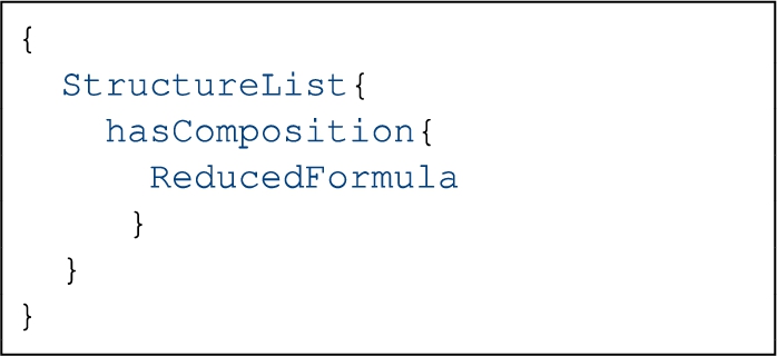
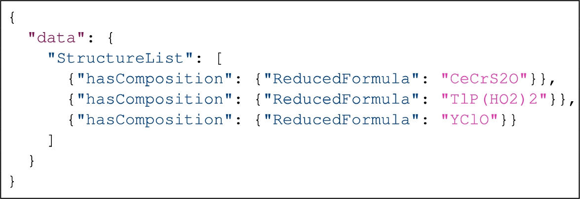
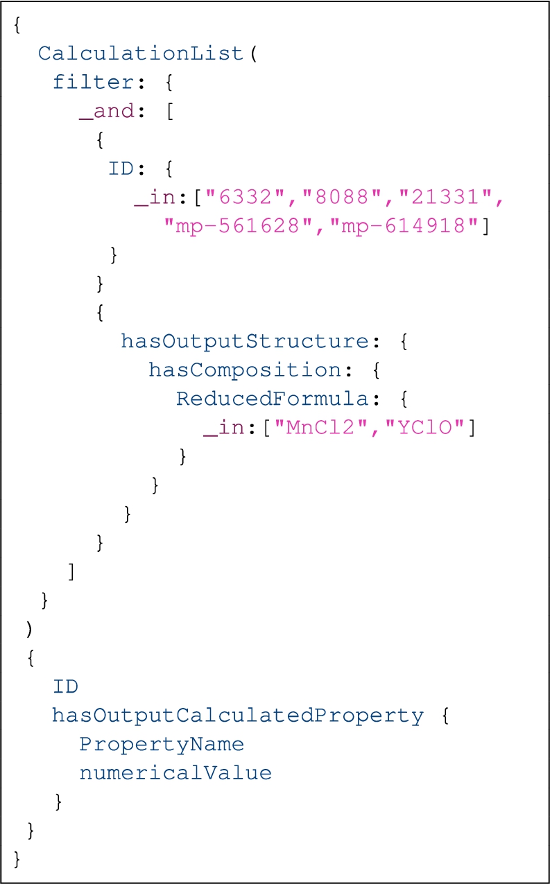
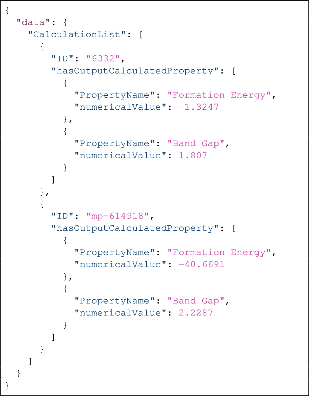
References
[1] | A. Agrawal and A. Choudhary, Perspective: Materials informatics and big data: Realization of the “fourth paradigm” of science in materials science, APL Materials 4: (053208) ((2016) ), 1–10. doi:10.1063/1.4946894. |
[2] | A. Alhazmi, T. Blount and G. Konstantinidis, ForBackBench: A benchmark for chasing vs. query-rewriting, in: Proceedings of the VLDB Endowment – 48th International Conference on Very Large Data Bases, Vol. 15: , Sydney, Australia, 2022, (2022) , pp. 1519–1532. doi:10.14778/3529337.3529338. |
[3] | C.W. Andersen, R. Armiento, E. Blokhin, G.J. Conduit, S. Dwaraknath, M.L. Evans, Á. Fekete, A. Gopakumar, S. Gražulis, A. Merkys, F. Mohamed, C. Oses, G. Pizzi, G.-M. Rignanese, M. Scheidgen, L. Talirz, C. Toher, D. Winston, R. Aversa, K. Choudhary, P. Colinet, S. Curtarolo, D. Di Stefano, C. Draxl, S. Er, M. Esters, M. Fornari, M. Giantomassi, M. Govoni, G. Hautier, V. Hegde, M.K. Horton, P. Huck, G. Huhs, J. Hummelshøj, A. Kariryaa, B. Kozinsky, S. Kumbhar, M. Liu, N. Marzari, A.J. Morris, A.A. Mostofi, K.A. Persson, G. Petretto, T. Purcell, F. Ricci, F. Rose, M. Scheffler, D. Speckhard, M. Uhrin, A. Vaitkus, P. Villars, D. Waroquiers, C. Wolverton, M. Wu and X. Yang, OPTIMADE: An API for exchanging materials data, Scientific Data 8: (217) ((2021) ). doi:10.1038/s41597-021-00974-z. |
[4] | Apollo Inc., Introduction to Apollo federation, accessed: 2022-07-29, https://www.apollographql.com/docs/federation/. |
[5] | M. Arenas, A. Bertails, E. Prud’hommeaux and J. Sequeda, A direct mapping of relational data to RDF, accessed, 2022-07-29, https://www.w3.org/TR/rdb-direct-mapping/. |
[6] | J. Arenas-Guerrero, D. Chaves-Fraga, J. Toledo, M.S. Pérez and O. Corcho, Morph-KGC: Scalable knowledge graph materialization with mapping partitions, Semantic Web ((2022) ). doi:10.3233/SW-223135. |
[7] | F. Baader, D. Calvanese, D.L. McGuinness, D. Nardi and P.F. Patel-Schneider, The Description Logic Handbook: Theory, Implementation and Applications, 2nd edn, Cambridge University Press, (2007) . doi:10.1017/CBO9780511711787. |
[8] | F. Baader, O.F. Gil and M. Pensel, Standard and non-standard inferences in the description logic FL0 using tree automata, in: GCAI-2018. 4th Global Conference on Artificial Intelligence, Vol. 55: , (2018) , pp. 1–14. doi:10.29007/scbw. |
[9] | F. Baader, I. Horrocks, C. Lutz and U. Sattler, An Introduction to Description Logic, 1st edn, Cambridge University Press, (2017) . doi:10.1017/9781139025355. |
[10] | F. Baader, P. Marantidis and M. Pensel, The data complexity of answering instance queries in FL0, in: Companion Proceedings of the Web Conference 2018, WWW ’18, International World Wide Web Conferences Steering Committee, (2018) , pp. 1603–1607. doi:10.1145/3184558.3191618. |
[11] | B. Bhattacharya, An introduction to GraphQL federation, accessed: 2022-07-29, https://tyk.io/blog/an-introduction-to-graphql-federation/. |
[12] | A.S.C. Bizer, The Berlin SPARQL benchmark, International Journal on Semantic Web and Information Systems (IJSWIS) 5: (2) ((2009) ), 11. doi:10.4018/jswis.2009040101. |
[13] | D. Calvanese, B. Cogrel, S. Komla-Ebri, R. Kontchakov, D. Lanti, M. Rezk, M. Rodriguez-Muro and G. Xiao, Ontop: Answering SPARQL queries over relational databases, Semantic Web 8: (3) ((2017) ), 471–487. doi:10.3233/SW-160217. |
[14] | D. Calvanese and G. De Giacomo, Data integration: A logic-based perspective, AI Magazine 26: (1) ((2005) ), 59–59. doi:10.1609/aimag.v26i1.1799. |
[15] | D. Calvanese, G.D. Giacomo, D. Lembo, M. Lenzerini and R. Rosati, Ontology-based data access and integration, in: Encyclopedia of Database Systems, Springer, New York, NY, (2018) , pp. 2590–2596. doi:10.1007/978-1-4614-8265-9_80667. |
[16] | J.J. Carroll, I. Dickinson, C. Dollin, D. Reynolds, A. Seaborne and K. Wilkinson, Jena: Implementing the semantic web recommendations, in: Proceedings of the 13th International World Wide Web Conference on Alternate Track Papers & Posters, Association for Computing Machinery, (2004) , pp. 74–83. doi:10.1145/1013367.1013381. |
[17] | D. Chaves-Fraga, F. Priyatna, A. Alobaid and O. Corcho, Exploiting declarative mapping rules for generating GraphQL servers with Morph-GraphQL, International Journal of Software Engineering and Knowledge Engineering 30: (06) ((2020) ), 785–803. doi:10.1142/S0218194020400070. |
[18] | D. Chaves-Fraga, F. Priyatna, A. Cimmino, J. Toledo, E. Ruckhaus and O. Corcho, GTFS-Madrid-Bench: A benchmark for virtual knowledge graph access in the transport domain, Journal of Web Semantics 65: ((2020) ), 100596. doi:10.1016/j.websem.2020.100596. |
[19] | D. Chaves-Fraga, E. Ruckhaus, F. Priyatna, M. Vidal and O. Corcho, Enhancing virtual ontology based access over tabular data with Morph-CSV, Semantic Web 12: (6) ((2021) ), 869–902. doi:10.3233/SW-210432. |
[20] | S. Cheng and O. Hartig, LinGBM: A performance benchmark for approaches to build GraphQL servers, in: Web Information Systems Engineering – WISE 2022 – 23rd International Conference on Web Information Systems Engineering, Biarritz, France, 2022, Lecture Notes in Computer Science, Vol. 13724: , Springer, Cham, (2022) , pp. 1–3. doi:10.1007/978-3-031-20891-1_16. |
[21] | O. Corcho, F. Priyatna and D. Chaves-Fraga, Towards a new generation of ontology based data access, Semantic Web 11: (1) ((2020) ), 153–160. doi:10.3233/SW-190384. |
[22] | S. Das, S. Sundara and R. Cyganiak, R2RML: RDB to RDF mapping language, accessed: 2022-07-29, https://www.w3.org/TR/r2rml/. |
[23] | B. De Meester, T. Seymoens, A. Dimou and R. Verborgh, Implementation-independent function reuse, Future Generation Computer Systems 110: ((2020) ), 946–959. doi:10.1016/j.future.2019.10.006. |
[24] | A. Dimou, M. Vander Sande, P. Colpaert, R. Verborgh, E. Mannens and R. Van de Walle, RML: A generic language for integrated RDF mappings of heterogeneous data, in: Proceedings of the Workshop on Linked Data on the Web Co-Located with the 23rd International World Wide Web Conference (WWW 2014), CEUR Workshop Proceedings, Vol. 1184: , (2014) , http://ceur-ws.org/Vol-1184/ldow2014_paper_01.pdf. |
[25] | A. Dimou, M. Vander Sande, J. Slepicka, P. Szekely, E. Mannens, C. Knoblock and R. Van de Walle, Mapping hierarchical sources into RDF using the RML mapping language, in: 2014 IEEE International Conference on Semantic Computing, (2014) , pp. 151–158. doi:10.1109/ICSC.2014.25. |
[26] | A. Doan, A. Halevy and Z. Ives, 1 – Introduction, in: Principles of Data Integration, Morgan Kaufmann, (2012) , pp. 1–18. doi:10.1016/B978-0-12-416044-6.00001-6. |
[27] | C. Draxl and M. Scheffler, NOMAD: The FAIR concept for big data-driven materials science, MRS Bulletin 43: (9) ((2018) ), 676–682. doi:10.1557/mrs.2018.208. |
[28] | K.M. Endris, P.D. Rohde, M.-E. Vidal and S. Auer, Ontario: Federated query processing against a semantic data lake, in: Database and Expert Systems Applications – 30th International Conference, DEXA 2019, Linz, Austria, August 26–29, 2019, Lecture Notes in Computer Science, Vol. 11706: , Springer, Cham, (2019) , pp. 379–395. doi:10.1007/978-3-030-27615-7_29. |
[29] | Facebook Inc., Specification for GraphQL – June 2020 edition, accessed: 2022-07-29, http://spec.graphql.org/draft/. |
[30] | C. Farré, J. Varga and R. Almar, GraphQL schema generation for data-intensive web APIs, in: Model and Data Engineering – 9th International Conference, MEDI 2019, Toulouse, France, October 28–31, 2019, Lecture Notes in Computer Science, Vol. 11815: , Springer, Cham, (2019) , pp. 184–194. doi:10.1007/978-3-030-32065-2_13. |
[31] | D. Garijo and M. Osorio, OBA: An ontology-based framework for creating REST APIs for knowledge graphs, in: The Semantic Web – ISWC 2020 – 19th International Semantic Web Conference, Athens, Greece, November 2–6, 2020, Lecture Notes in Computer Science, Vol. 12507: , Springer, Cham, (2020) , pp. 48–64. doi:10.1007/978-3-030-62466-8_4. |
[32] | L. Gleim, T. Holzheim, I. Koren and S. Decker, Automatic bootstrapping of GraphQL endpoints for RDF triple stores, in: Proceedings of the QuWeDa 2020: 4th Workshop on Querying and Benchmarking the Web of Data Co-Located with 19th International Semantic Web Conference (ISWC 2020), CEUR Workshop Proceedings, Vol. 2722: , CEUR-WS, (2020) , pp. 119–134, http://ceur-ws.org/Vol-2722/quweda2020-paper-2.pdf. |
[33] | O. Hartig and J. Hidders, Defining schemas for property graphs by using the GraphQL schema definition language, in: Proceedings of the 2nd Joint International Workshop on Graph Data Management Experiences & Systems (GRADES) and Network Data Analytics (NDA) Co-Located with SIGMOD/PODS ’19: International Conference on Management of Data, GRADES-NDA’19, Association for Computing Machinery, (2019) , pp. 1–11. doi:10.1145/3327964.3328495. |
[34] | O. Hartig and J. Pérez, Semantics and complexity of GraphQL, in: Proceedings of the 2018 World Wide Web Conference, WWW ’18, International World Wide Web Conferences Steering Committee, (2018) , pp. 115–1164. doi:10.1145/3178876.3186014. |
[35] | I. Horrocks, P.F. Patel-Schneider and F. Van Harmelen, From SHIQ and RDF to OWL: The making of a web ontology language, Journal of Web Semantics 1: (1) ((2003) ), 7–26. doi:10.1016/j.websem.2003.07.001. |
[36] | I. Horrocks and U. Sattler, Ontology reasoning in the SHOQ(d) description logic, in: Proceedings of the 17th International Joint Conference on Artificial Intelligence, IJCAI’01, Vol. 1: , Morgan Kaufmann Publishers Inc., (2001) , pp. 199–204. doi:10.5555/1642090.1642117. |
[37] | A. Jain, S.P. Ong, G. Hautier, W. Chen, W.D. Richards, S. Dacek, S. Cholia, D. Gunter, D. Skinner, G. Ceder and K.A. Persson, The materials project: A materials genome approach to accelerating materials innovation, APL Materials 1: (1) ((2013) ), 011002. doi:10.1063/1.4812323. |
[38] | S.R. Kalidindi and M. De Graef, Materials data science: Current status and future outlook, Annual Review of Materials Research 45: ((2015) ), 171–193. doi:10.1146/annurev-matsci-070214-020844. |
[39] | S. Karcher, E.L. Willighagen, J. Rumble, F. Ehrhart, C.T. Evelo, M. Fritts, S. Gaheen, S.L. Harper, M.D. Hoover, N. Jeliazkova, N. Lewinski, R.L.M. Robinson, K.C. Mills, A.P. Mustad, D.G. Thomas, G. Tsiliki and C.O. Hendren, Integration among databases and data sets to support productive nanotechnology: Challenges and recommendations, NanoImpact 9: ((2018) ), 85–101. doi:10.1016/j.impact.2017.11.002. |
[40] | P. Lambrix, R. Armiento, A. Delin and H. Li, Big semantic data processing in the materials design domain, in: Encyclopedia of Big Data Technologies, Springer, Cham, (2019) . doi:10.1007/978-3-319-63962-8_293-1. |
[41] | P. Lambrix, R. Armiento, A. Delin and H. Li, FAIR big data in the materials design domain, in: Encyclopedia of Big Data Technologies, Springer, Cham, (2022) . doi:10.1007/978-3-319-63962-8_293-2. |
[42] | D. Lanti, M.I. Rezk, G. Xiao and D. Calvanese, The NPD benchmark: Reality check for OBDA systems, in: Advances in Database Technology – EDBT 2015, 18th International Conference on Extending Database Technology, Brussels, Belgium, March 23–27, 2015, (2015) , pp. 617–628, OpenProceedings.org. doi:10.5441/002/edbt.2015.62. |
[43] | M. Lenzerini, Data integration: A theoretical perspective, in: Proceedings of the Twenty-First ACM SIGMOD-SIGACT-SIGART Symposium on Principles of Database Systems, PODS ’02, Association for Computing Machinery, (2002) , pp. 233–246. doi:10.1145/543613.543644. |
[44] | H. Li, Ontology-driven data access and data integration with an application in the materials design domain, PhD thesis, Linköping University, Sweden, (2022) . doi:10.3384/9789179292683. |
[45] | H. Li, R. Armiento and P. Lambrix, An ontology for the materials design domain, in: The Semantic Web – ISWC 2020 – 19th International Semantic Web Conference, Athens, Greece, November 2–6, 2020, Lecture Notes in Computer Science, Vol. 12507: , Springer, Cham, (2020) , pp. 212–227. doi:10.1007/978-3-030-62466-8_14. |
[46] | H. Li, O. Hartig, R. Armiento and P. Lambrix, OBG-gen: Ontology-based GraphQL server generation for data integration, in: Proceedings of the ISWC 2023 Posters & Demonstrations, Industry Tracks Co-Located with 22nd International Semantic Web Conference (ISWC 2023), CEUR Workshop Proceedings, CEUR-WS, (2023) . |
[47] | M.N. Mami, D. Graux, S. Scerri, H. Jabeen, S. Auer and J. Lehmann, Squerall: Virtual ontology-based access to heterogeneous and large data sources, in: The Semantic Web – ISWC 2019 –18th International Semantic Web Conference, Auckland, New Zealand, October 26–30, 2019, Lecture Notes in Computer Science, Vol. 11779: , Springer, Cham, (2019) , pp. 229–245. doi:10.1007/978-3-030-30796-7_15. |
[48] | G. Meditskos and N. Bassiliades, DLEJena: A practical forward-chaining OWL 2 RL reasoner combining Jena and Pellet, Journal of Web Semantics 8: (1) ((2010) ), 89–94. doi:10.1016/j.websem.2009.11.001. |
[49] | Morph-RDB, version 3.12.5, accessed: 2022-07-29, https://github.com/oeg-upm/morph-rdb/releases/tag/v3.12.5. |
[50] | Ontop, version 4.2.1, accessed: 2022-07-29, https://github.com/ontop/ontop/releases/tag/ontop-4.2.1. |
[51] | A. Poggi, D. Lembo, D. Calvanese, G. De Giacomo, M. Lenzerini and R. Rosati, Linking data to ontologies, Journal on Data Semantics X ((2008) ), 133–173. doi:10.1007/978-3-540-77688-8_5. |
[52] | F. Priyatna, O. Corcho and J. Sequeda, Formalisation and experiences of R2RML-based SPARQL to SQL query translation using Morph, in: Proceedings of the 23rd International Conference on World Wide Web, WWW ’14, Association for Computing Machinery, (2014) , pp. 479–490. doi:10.1145/2566486.2567981. |
[53] | J. Rumble, J. Broome and S. Hodson, Building an international consensus on multi-disciplinary metadata standards: A CODATA case history in nanotechnology, Data Science Journal 8: (12) ((2019) ), 1–11. doi:10.5334/dsj-2019-012. |
[54] | J.E. Saal, S. Kirklin, M. Aykol, B. Meredig and C. Wolverton, Materials design and discovery with high-throughput density functional theory: The Open Quantum Materials Database (OQMD), JOM 65: ((2013) ), 1501–1509. doi:10.1007/s11837-013-0755-4. |
[55] | Semantic Integration Ltd., HyperGraphQL, version 2.0.0, accessed: 2022-07-29, https://github.com/hypergraphql/hypergraphql/releases/tag/2.0.0. |
[56] | Semantic Integration Ltd., UltraGraphQL, version 1.0.0, accessed: 2022-07-29, https://git.rwth-aachen.de/i5/ultragraphql. |
[57] | B. Smith, Ontology, in: The Furniture of the World, Brill, (2012) , pp. 47–68. doi:10.1163/9789401207799_005. |
[58] | R. Stevens, C.A. Goble and S. Bechhofer, Ontology-based knowledge representation for bioinformatics, Briefings in Bioinformatics 1: (4) ((2000) ), 398–414. doi:10.1093/bib/1.4.398. |
[59] | R. Studer, V.R. Benjamins and D. Fensel, Knowledge engineering: Principles and methods, Data & Knowledge Engineering 25: (1) ((1998) ), 161–197. doi:10.1016/S0169-023X(97)00056-6. |
[60] | R. Taelman, M. Vander Sande and R. Verborgh, GraphQL-LD: Linked data querying with GraphQL, in: Proceedings of the ISWC 2018 Posters & Demonstrations, Industry and Blue Sky Ideas Tracks Co-Located with 17th International Semantic Web Conference (ISWC 2018), CEUR Workshop Proceedings, Vol. 2180: , CEUR-WS, (2018) , http://ceur-ws.org/Vol-2180/paper-65.pdf. |
[61] | A. Tropsha, K.C. Mills and A.J. Hickey, Reproducibility, sharing and progress in nanomaterial databases, Nature Nanotechnology 12: ((2017) ), 1111–1114. doi:10.1038/nnano.2017.233. |
[62] | D. Van Assche, T. Delva, G. Haesendonck, P. Heyvaert, B. De Meester and A. Dimou, Declarative RDF graph generation from heterogeneous (semi-)structured data: A systematic literature review, Journal of Web Semantics 75: ((2023) ), 100753. doi:10.1016/j.websem.2022.100753. |
[63] | P. Vassiliadis, A survey of extract-transform-load technology, integrations of data warehousing, data mining and database technologies, Innovative Approaches 5: (3) ((2009) ), 1–27. doi:10.4018/978-1-60960-537-7.ch008. |
[64] | C. Welty, Ontology research, AI Magazine 24: (3) ((2003) ), 11. doi:10.1609/aimag.v24i3.1714. |
[65] | G. Wiederhold, Mediators in the architecture of future information systems, Computer 25: (3) ((1992) ), 38–49. doi:10.1109/2.121508. |
[66] | G. Xiao, D. Calvanese, R. Kontchakov, D. Lembo, A. Poggi, R. Rosati and M. Zakharyaschev, Ontology-based data access: A survey, in: Proceedings of the Twenty-Seventh International Joint Conference on Artificial Intelligence, IJCAI-18, International Joint Conferences on Artificial Intelligence Organization, (2018) , pp. 5511–5519. doi:10.24963/ijcai.2018/777. |
[67] | G. Xiao, D. Hovland, D. Bilidas, M. Rezk, M. Giese and D. Calvanese, Efficient ontology-based data integration with canonical IRIs, in: The Semantic Web 15th International Conference, ESWC 2018, Heraklion, Crete, Greece, June 3–7, 2018, Proceedings, Lecture Notes in Computer Science, Vol. 10843: , Springer, Cham, (2018) , pp. 697–713. doi:10.1007/978-3-319-93417-4_45. |


