
Microsaccade dysfunction and adaptation in hemianopia after stroke
Abstract
Background:
Besides the reduction of visual field size, hemianopic patients may also experience other poorly understood symptoms such as blurred vision, diplopia, or reduced visual acuity, which may be related to microsaccade function.
Objective:
To determine (i) if microsaccades are altered in hemianopia; (ii) how altered microsaccade features correlate with visual performances; and (iii) how their direction relates to visual field defect topography.
Methods:
In this case-control study, microsaccades of hemianopic stroke patients (n = 14) were assessed with high-resolution eye-tracking technique, compared with those of healthy controls (n = 14), and correlated with visual performances, visual field defect parameters and lesion age.
Results:
Patients’ microsaccades had (i) larger amplitude (P = 0.027), (ii) longer duration (P = 0.042), and (iii) impaired binocular microsaccade conjugacy (horizontal: P = 0.002; vertical: P = 0.035). Older lesions were associated with poorer binocular conjugacy (horizontal: r(14) = 0.67, P = 0.009; vertical: r(14) = 0.75, P = 0.002) and larger microsaccade amplitudes (r(14) = 0.55, P = 0.043). (iv) Half of the patients had a microsaccade bias towards the seeing field (monocular: P = 0.002; binocular: P < 0.001) which was associated with faster reactions to super-threshold visual stimuli in areas of residual vision (P = 0.042). Finally, (v) patients with more binocular microsaccades (r(14) = 0.59, P = 0.027) and lower microsaccade velocity (r(14) = –0.66, P = 0.011) had better visual acuity.
Conclusions:
Hemianopia leads not only to the loss of visual field but also to microsaccade enlargement and impaired binocular conjugacy, suggesting malfunctioning microsaccade control circuits which worsen over time. But a microsaccade bias towards the seeing field, which suggests greater allocation of attention, accelerates stimulus detection. Microsaccades may play a role to compensate for vision impairment and provide a basis for vision restoration and plasticity, which deserves further exploration.
Abbreviation
ARVs | areas of residual vision |
dCX | horizontal disconjugacy index |
dCY | vertical disconjugacy index |
HRP | high-resolution computer-based perimetry |
SC | superior colliculus |
1Introduction
One cause of vision loss is brain stroke or trauma, leading to homonymous hemianopia (Rowe et al., 2009; Sand et al., 2013). While visual field defects in hemianopia can be well characterized with perimetry, visual field size and topography correlate poorly with vision-related quality of life (Gall et al., 2010; Gall et al., 2009; Gall et al., 2008; Papageorgiou et al., 2007). Besides the reduction of visual field size, patients may also experience other still poorly understood symptoms such as blurred vision, diplopia, or reduced visual acuity which is independent of the eye’s optics (de Haan et al., 2015; D. Poggel et al., 2007; Rowe et al., 2013). And there are even deficits in the “intact” field (“sightblindness”) (Bola et al., 2013a, 2013b). One important contributor to these visual impairments may be microsaccades which are tiny but essential for normal vision (Martinez-Conde et al., 2013). The reasons why we suspected microsaccade alterations in hemianopia are two-fold: (i) altered microsaccades can cause blurred (foggy) vision and low visual acuity (Ciuffreda & Tannen, 1995; Foroozan & Brodsky, 2004), which were reported in hemianopia (Rowe et al., 2013); (ii) microsaccades are controlled by a complex brain functional connectivity network involving the superior colliculus (SC) (Hafed et al., 2009), multiple eye fields, and visual cortex (Lynch, 2009). Since brain functional connectivity alterations were reported in vision loss well beyond the local lesion (Bola et al., 2014; Bola et al., 2015), we suspected that even brain regions located at some distance from the lesion (such as the frontal eye fields) may be affected, disturbing microsaccades in hemianopia.
In this case-control study, we compared microsaccade features in hemianopia to those in healthy controls and correlated them with visual performances and lesion age. Based on prior reports, we expected three altered microsaccade features in hemianopia: (i) enlarged microsaccade amplitude due to a decreased inhibition of the SC after visual deafferentation (Shi et al., 2012); (ii) reduced binocular microsaccade conjugacy due to miscalibration of the eye movement control network after visual input deprivation (Schneider et al., 2013); and (iii) microsaccade direction bias towards the deficit side, similar to those changes reported in hemianopia (Reinhard et al., 2014).
2Methods
2.1Protocol approvals, registration, and patient consent
Written informed consent was obtained from all participants according to the Declaration of Helsinki (International Committee of Medical Journal Editors, 1991) after the institutional review board approved the study protocol.
2.2Participants and study design
For this case-control study 14 patients with homonymous hemianopia including incomplete hemianopia (13 male/1 female; mean age: 59, range from 45 to 73) and 14 healthy controls (11 male/3 female; mean age: 60, range from 44 to 71) were recruited and tested from February 2014 to September 2015. Both groups did not differ in age (t(26) = –0.13, P = 0.897). Table 1 shows the patients’ demographic and medical characteristics.
Table 1
Patients’ demographic and medical characteristics
| Patient | Age (year) | Gender | Lesion age | Cause of damage | Visual field defect |
| (month) | |||||
| 01 | 45 | male | 61 | Left PCA infarct | right upper quadrantanopia |
| 02 | 65 | male | 20 | Left PCA infarct | right lower quadrantanopia |
| 03 | 68 | male | 45 | Right OL ischemia | left hemianopia |
| 04 | 73 | male | 19 | Left PCA infarct | right hemianopia |
| 05 | 62 | male | 28 | Left PCA infarct | right hemianopia |
| 06 | 52 | male | 29 | Right PCA infarct | left upper quadrantanopia |
| 07 | 49 | male | 11 | Right PCA infarct | left hemianopia |
| 08 | 66 | male | 49 | Right PCA infarct | left hemianopia |
| 09 | 72 | male | 19 | Right OL stroke | left lower quadrantanopia |
| 10 | 45 | male | 43 | Right PCA infarct | left hemianopia |
| 11 | 53 | male | 93 | Left OL stroke | right hemianopia |
| 12 | 58 | male | 6 | Left OL infarct | right hemianopia and |
| left upper quadrantanopia | |||||
| 13 | 61 | male | 6 | Right PCA and PICA infarct | left hemianopia |
| 14 | 60 | female | 7 | Right PCA infarct | left lower quadrantanopia |
Abbreviations: PCA = posterior cerebral artery; OL = occipital lobe; PICA = posterior inferior cerebellar artery.
Inclusion criteria: hemianopia after posterior artery stroke-related occipital cortex damage with lesion age ≥6 months. Exclusion criteria: complete blindness, visual hemi-neglect, psychiatric diseases (schizophrenia etc.), serious substance abuse, diabetic retinopathy or diabetes mellitus with average blood glucose level above 7 mmol/l, blood pressure instable and >160/100 mmHg, instable or high level of intraocular pressure (>27 mm of hg column), retinitis pigmentosa, pathological nystagmus, and any ophthalmological disorder affecting visual functions.
2.3Eye movement recording
Binocular eye movements were recorded during a fixation task using an EyeLink-1000 system (SR Research, Ontario, Canada) with a sampling rate of 500 Hz. During the fixation task, participants were instructed to maintain fixation at a fixation dot on a gamma corrected monitor (EIZO, CG241W, resolution of 2560×1440) which was placed at 67 cm distance. The white fixation dot (size: 10 pixels, luminance: 90 cd/m2) was presented against grey background (luminance: 29 cd/m2) in 40 trials lasting 7 sec each. The inter-stimulus interval was 3 sec, during which participants could rest their eyes. Participants were tested individually in a silent, dimly lit room with their head fixed by a chin rest during eye tracker calibration, validation and recording.
2.4Visual performances
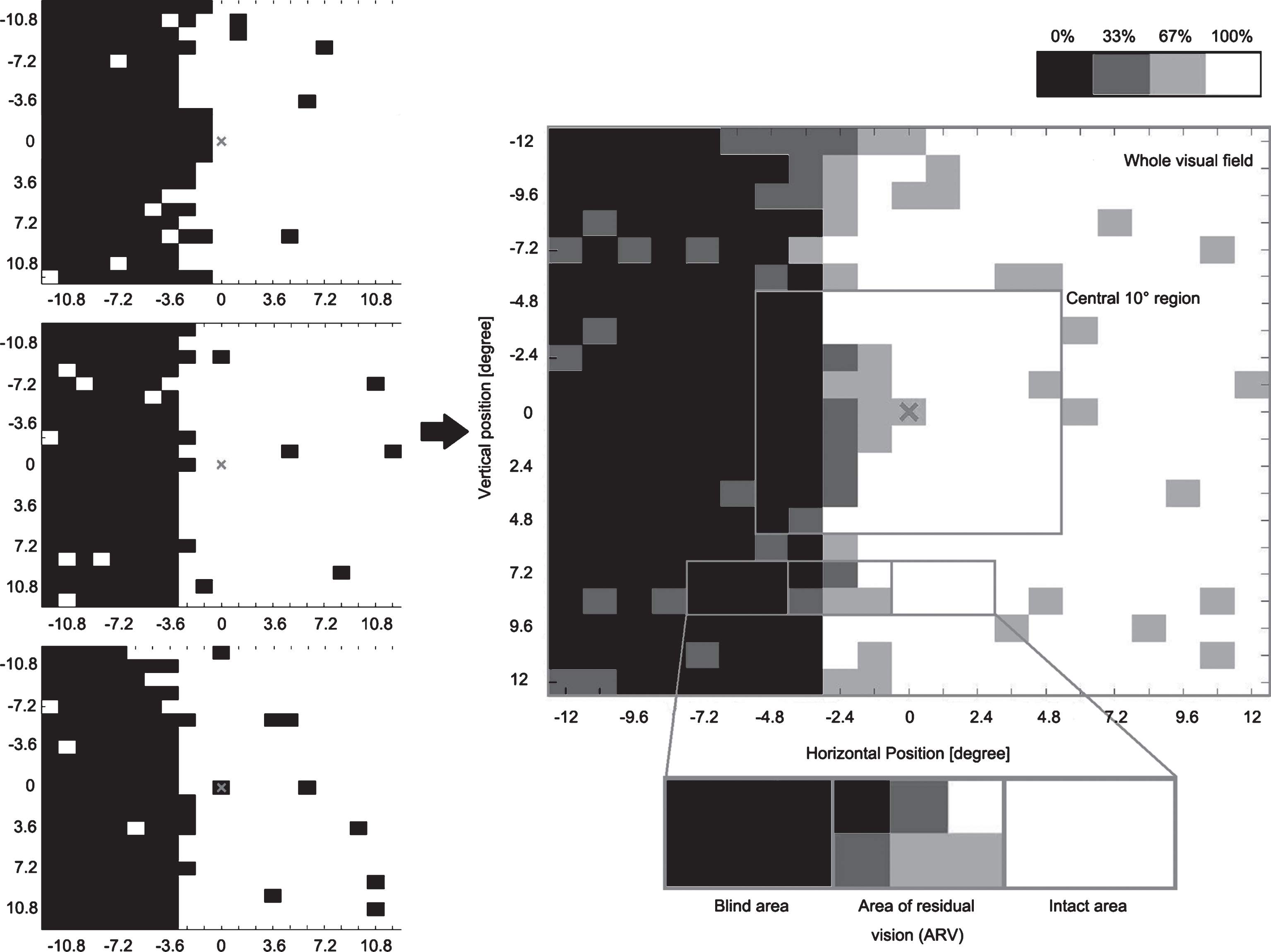
Visual acuity was measured with the standard Landolt ‘C’ test at a 40 cm distance (Standard-Snellen, with see-chart from Oculus), contrast sensitivity with the MARS contrast chart (MARS Perceptrix Corporation), dynamic vision performance with Düsseldorf Dynamic Vision Test, and visual fields parameters with a high-resolution computer-based campimetric visual field test with super-threshold stimuli (High-Resolution computer-based Perimetry, HRP; Fig. 1) (Sabel et al., 2004). For HRP, we analyzed the size of blind areas and areas of residual vision (ARVs) in the whole visual field (covering 25°x25° of subjects’ visual field), response time in the whole visual field, in intact areas and in ARVs. Figure 1 illustrates how we define the central 10° by 10° region, blind areas, ARVs and intact areas.
Fig.1
Visual area categorization based on visual field chart from high-resolution computer-based perimetry (HRP). During HRP, a supra-threshold stimulus detection task was carried out three times, creating three simple detection charts (left column). The white area shows the intact visual field, while the black area shows blind regions. By superimposing these three detection charts, we obtained a new visual chart (right center). The emerging grey area represents visual field sectors where patients’ response accuracy was inconsistent; with light grey representing the area where patients responded to 2/3 targets and dark grey represents areas with 1/3 response. All grey areas together are defined as “areas of residual vision” (ARVs). The black areas and the white areas were defined as being blind or intact, respectively. We also analyzed the central square region 10° by 10°.
2.5Eye movement data analysis
2.5.1Microsaccade detection
Microsaccade detection was based on published algorithms (Engbert & Kliegl, 2003; Engbert & Mergenthaler, 2006) and programmed in Matlab (Mathworks, Massachusetts, U.S.A). The time series of eye positions were transformed to velocities by calculating a moving average of velocities over five data samples. A microsaccade was defined by the following criteria: (i) the velocity exceeded six median-based standard deviations of the velocity distribution; (ii) the duration exceeds 12 msec (6 data samples); (iii) the inter-saccadic interval exceeded 24 msec (12 data samples). The criterion to confirm microsaccade detection validity was the main sequence relationship between microsaccade amplitude and microsaccade velocity (Zuber et al., 1965). Microsaccade features we analyzed were rate (microsaccade number devided by detection time window length), amplitude (the Euclidean distance between the start and end point of the movement), velocity (the peak velocity during one microsaccade) and duration.
2.5.2Conjugacy analysis
Binocular microsaccades were defined as those that occurred in left and right eyes with a temporal overlap as defined by Engbert and Kliegl (Engbert & Kliegl, 2003). After detection of these binocular microsaccades, binocular microsaccade percentage was calculated as the proportion of binocular microsaccades in all detected microsaccades.
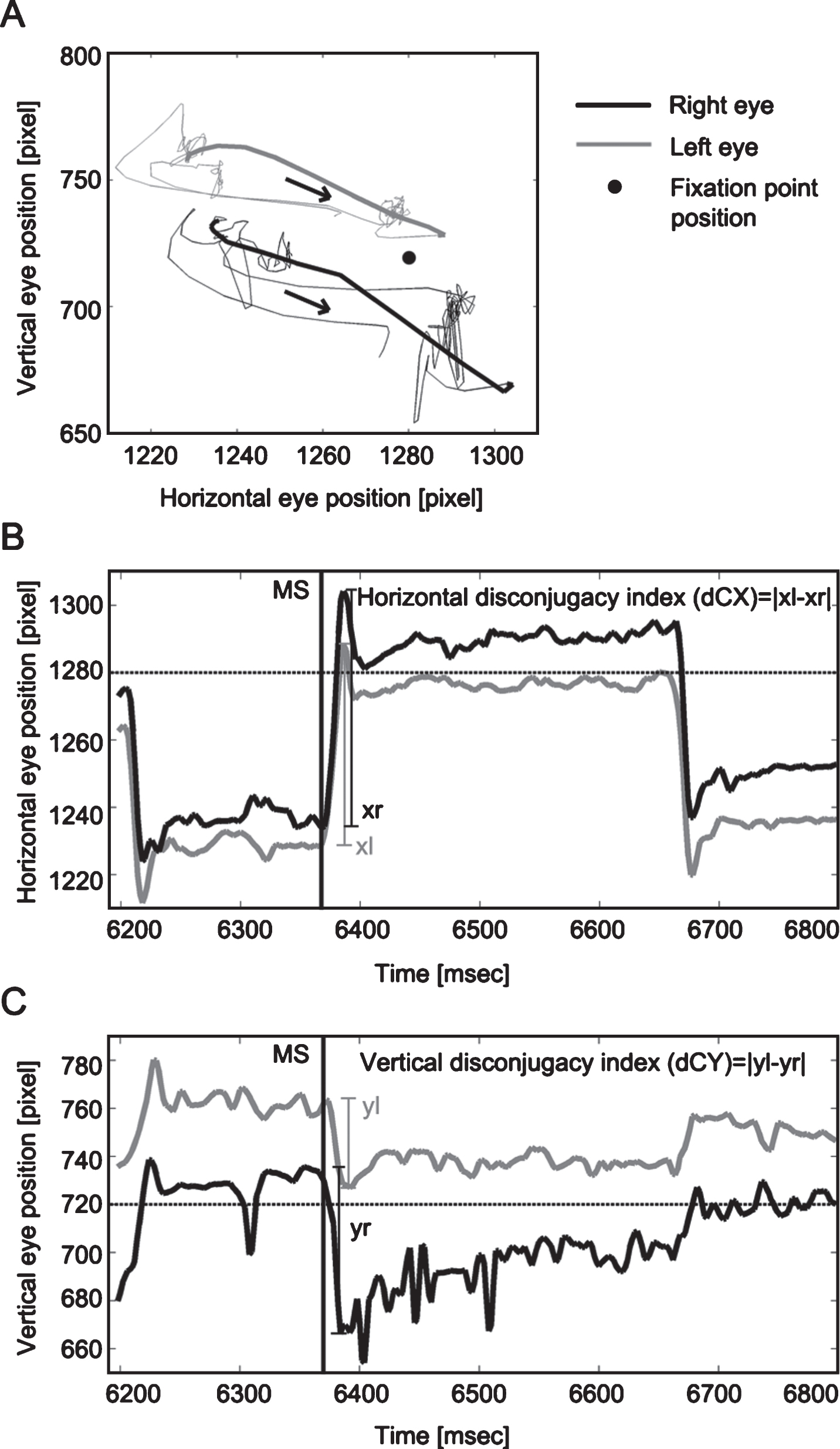
We paired the microsaccades from the two eyes in each overlapped time window and resolved each microsaccade into one horizontal component x and one vertical component y. For each pair of eyes we defined two components for the left (xl and yl) and right eye (xr and yr) to calculate the disconjugacy indices using the following equations:
(1)
(2)
Larger values of these two indices represent larger discrepancy between the two eyes, indicating poorer binocular conjugacy (Fig. 2). Thus, we obtained binocular microsaccade percentage, dCX and dCY for each subject.
Fig.2
Trajectory (A), horizontal (B) and vertical (C) binocular disconjugacy indices of one microsaccade. Panel A presents the trajectory of one microsaccade (bold lines). The black arrows indicate the moving direction of the microsaccade. Panels B and C illustrate the calculation of horizontal (dCX) and vertical disconjugacy index (dCY) for this pair of binocular microsaccades. Left and right eye movements are represented by grey or black solid lines, respectively; the fixation point position is represented by the horizontal dotted lines (in B and C) or black dot (in A). Black solid vertical lines (in B and C) indicate the onset of one microsaccade (around 6360 ms). Larger values of dCX and dCY indicate larger discrepancies between two eyes, i.e. poorer binocular conjugacy.
2.5.3Classifying microsaccades based on their direction
In the hemianopia group, monocular and binocular microsaccades were classified as belonging to one of two categories according to their direction: bias towards the deficit or bias towards the intact hemifield. This direction bias was calculated as follows:
(3)
In incomplete hemianopia, when patients show no bias towards either field, microsaccade direction bias is susceptible to the area ratio of the deficit and intact areas. For convenience of inter-subject comparison, we calculated the microsaccade direction bias in incomplete hemianopia as follows:
(4)
2.6Statistical analysis
Independent-sample t tests were conducted to test the microsaccade feature differences between the heminopia group and the control group. Before conducting between-groups statistical tests, normality of distribution was assessed with Shapiro-Wilk test. For measures violating the normal distribution assumption, Mann-Whitney U test was used. One-sample t tests were performed to test the microsaccade direction bias against 1. A criterion of P = 0.05 (two-tailed) was set for all statistical tests. Bonferroni-Holm correction was performed to correct for multiple comparisons and are reported as Pcor. As this is the first explorative study on microsaccades in hemianopia, we also present the original p values and discussed the results as a reference for future studies.
Pearson’s correlations were calculated between patients’ microsaccade features (binocular microsaccade percentage, dCX, dCY, microsaccade rate, amplitude, velocity, duration, monocular and binocular microsaccade direction bias), lesion age, and visual performances (visual acuity, contrast sensitivity, dynamic vision performance, fixation accuracy during HRP, blind area and ARVs sizes in the whole visual field and central 10 ° region, mean response time in the intact visual field and ARVs). A bootstrapping method was utilized to reduce spurious findings (5000 samples, bias-corrected and accelerated 95% confidence interval).
Statistical analyses were performed using IBM SPSS Statistics 22 (IBM, USA, http://www.ibm.com/software/analytics/spss/) and R-Studio (version 0.99. 903, RStudio Team, USA, http://www.rstudio.com).
3Results
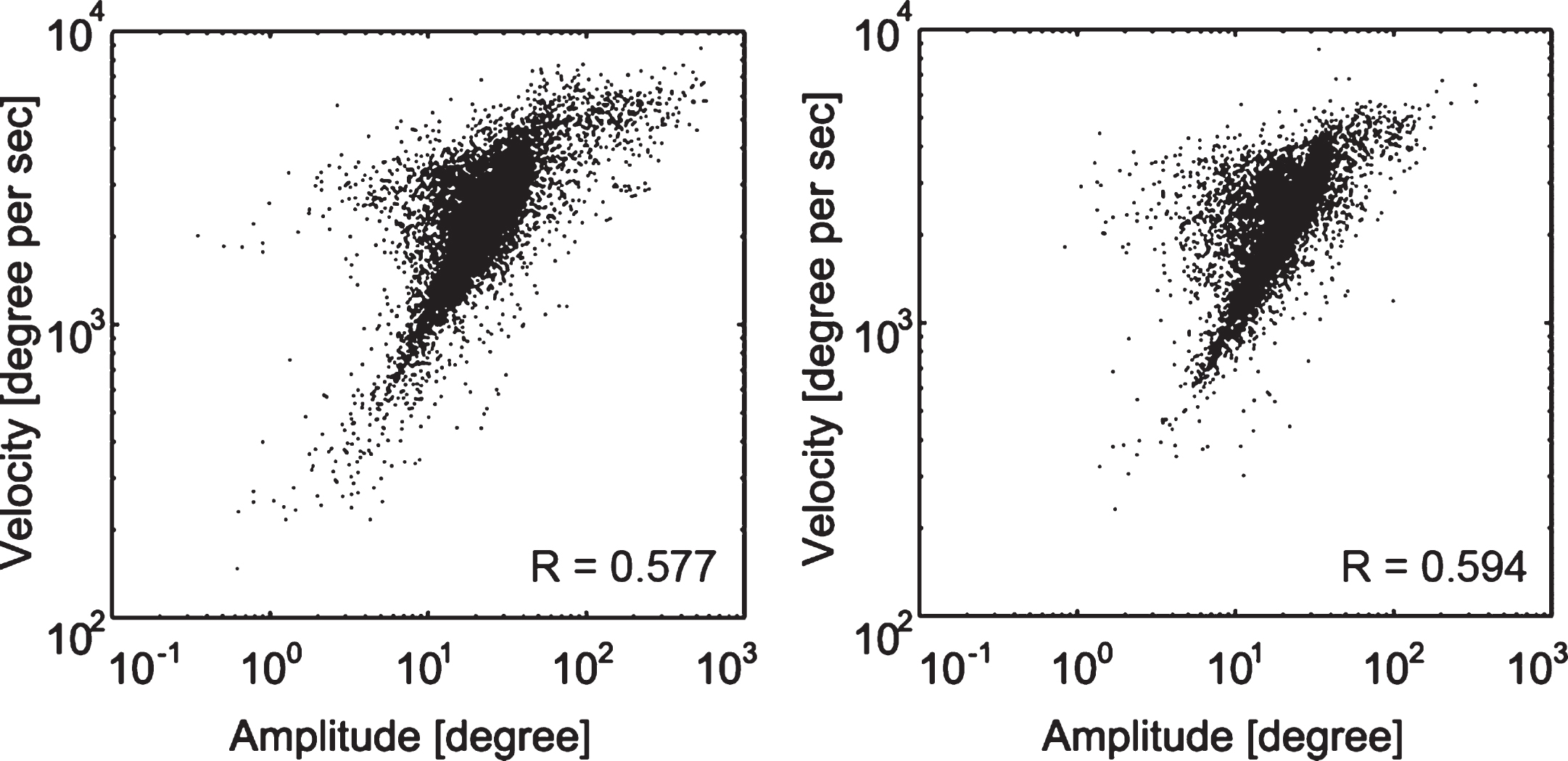
None of the participants dropped out from the study. After microsaccade detection and computation of microsaccade features, main sequences were generated for all microsaccades in both groups (Fig. 3).
Fig.3
Microsaccades main sequence. Main sequence for all microsaccades in the hemianopia (left) and control group (right). The humps toward the left in both groups’ main sequence graphs are due to the slope variance in subjects. The correlation coefficient R values are displayed for each group.
3.1Comparison between hemianopic patients and normal controls
Table 2 presents the summary of all microsaccade features and the statistics of the group differences. Consistent with our hypotheses, the hemianopia group displayed larger microsaccade amplitude and reduced horizontal and vertical binocular conjugacy. Hemianopic patients also exhibited longer microsaccade duration. The group difference in horizontal disconjugacy was significant even when Bonferroni-Holm correction was applied. No group difference was discovered in other microsaccade features such as rate, velocity, and binocular microsaccade percentage.
Table 2
Microsaccade features in hemianopia and control groups and the group differences
| Microsaccade | Hemianopic group | Control group | t | P | P cor | 95% confidence |
| features | (n = 14) | (n = 14) | interval | |||
| Amplitude (degree) | 0.46±0.03 | 0.38±0.02 | 2.34 | 0.027 | 0.162 | –0.009, 0.144 |
| Horizontal disconjugacy (min arc) | 10.39 (20.59)a | 8.01 (4.39)a | 31.00b | 0.002 | 0.014 | n/a |
| Vertical disconjugacy (min arc) | 9.62 (30.24)a | 7.57 (7.98)a | 52.00b | 0.035 | 0.175 | n/a |
| Binocular Microsaccade percentage (%) | 0.48±0.06 | 0.55±0.04 | –0.98 | 0.336 | 0.744 | –0.205, 0.072 |
| Microsaccade rate (num per sec) | 1.41±0.23 | 1.37±0.20 | 0.13 | 0.894 | 0.894 | –0.581, 0.663 |
| velocity (degree per sec) | 43.21±1.44 | 41.05±1.12 | 1.18 | 0.248 | 0.744 | –1.589, 5.894 |
| Duration (msec) | 17.64±0.92 | 15.42±0.44 | 2.18 | 0.042 | 0.175 | 0.086, 4.349 |
aNormal distributed microsaccade feature values are displayed as mean±SEM, while non-normal distributed feature values are displayed as median (range). bMann-Whitney U tests were performed and U values are presented here because the data was not normally distributed.
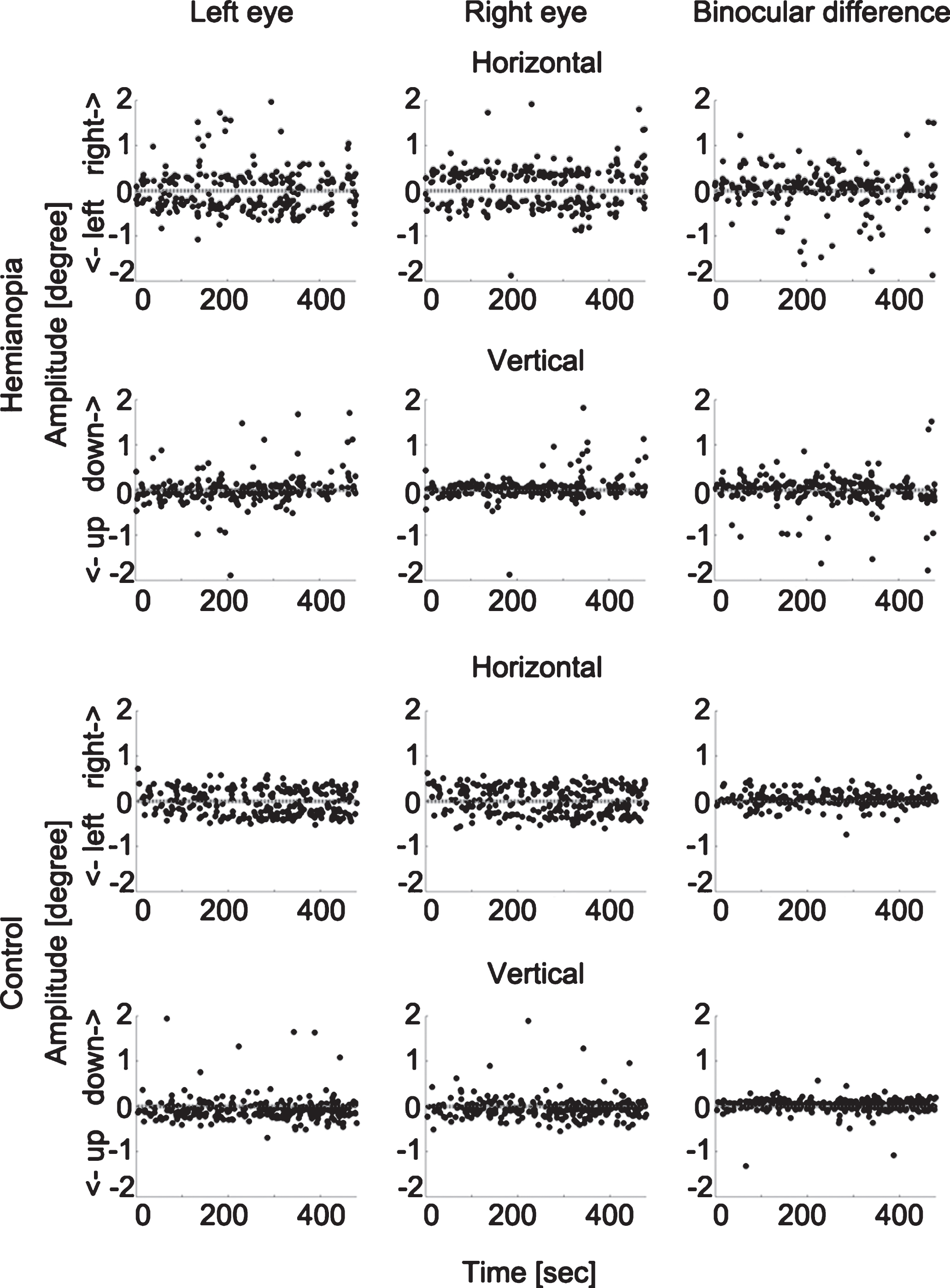
To rule out the possibility that such binocular disconjugacy was due to the differences in eye tracker calibration, we compared the binocular difference in calibration outcomes of the hemianopia and control groups with an independent sample two-tailed t test and found them to be comparable (hemianopia: mean = 0.14 deg, SEM = 0.06 deg; controls: mean = 0.06 deg, SEM = 0.01 deg; t(14.22) = 1.25, P = 0.230). Figure 4 displays examples of the binocular conjugacy patterns of one patient and one control subject.
Fig.4
Microsaccade binocular conjugacy patterns in one hemianopic patient and one control subject. The upper two rows show the horizontal and vertical microsaccade components of one participant with hemianopia and the binocular difference. The lower two rows display the same for one control subject. Each dot represents one microsaccade. The horizontal dotted lines represent the fixation point position. The hemianopic patient shows larger binocular difference, both in the horizontal and vertical directions.
3.2Microsaccade direction bias in hemianopia
One-sample t-test results showed that the hemianopia group’s monocular (mean = 0.89, SEM = 0.11) and binocular microsaccade direction bias (mean = 1.03, SEM = 0.24) were not significantly different from 1 (t(13) = –1.07, P = 0.304; t(13) = 0.13, P = 0.898).
Further examination of patients’ individual microsaccade distribution revealed that 7 of 14 patients showed a microsaccade direction bias towards the intact areas whereas the other seven did not have any bias, i.e. we found not a single case with a direction bias towards the hemianopic hemifield. To explore the difference between these two kinds of responses, we subdivided the hemianopia group into two subgroups: a biased and a non-biased group. Figure 5 illustrates their respective monocular and binocular microsaccade direction bias.
Fig.5
HRP visual charts, monocular and binocular microsaccade angular histograms of representative hemianopia cases of the biased (A) and the non-biased group (B). The HRP visual charts (first column) and angular histograms of monocular (second column) and binocular (third column) microsaccades from four patients with hemianopia (two in each subgroup) are presented. In the biased group, the angular histograms show more microsaccades towards the intact area. In the non-biased group, the angular histograms show no specific bias of microsaccade direction towards the blind or intact areas. Note: The angular histograms do not convey information about microsaccade amplitudes. Bar length rather represents microsaccade numbers.

To confirm that our selection led to distinct subgroups, we tested their microsaccade direction bias against 1. The results confirmed that both monocular and binocular microsaccades were towards the intact area in the biased group (monocular: mean = 0.66, SEM = 0.06, t(6) = –5.41, p = 0.002; binocular: mean = 0.41, SEM = 0.08, t(6) = –7.45, p < 0.001) while the non-biased group showed no specific bias (monocular: mean = 1.12, SEM = 0.16, t(6) = 0.73, p = 0.494; binocular: mean = 1.66, SEM = 0.33, t(6) = 2.02, p = 0.090).
Next we tested the subgroup differences in all microsaccade features, lesion age, visual field defect parameters and visual performances. The two subgroups differed in reaction time in ARVs: the biased group (mean = 0.50 sec, SEM = 0.02 sec) responded significantly faster to the visual stimuli than the non-biased group (mean = 0.56 sec, SEM = 0.03 sec; t(12) = –2.28, p = 0.042, pcor = 0.456). This observation suggests that a direction bias towards the seeing field is adaptive and facilitates visual processing. However, this difference did not reach the significance level after Bonferroni-Holm correction for multiple comparison and the interpretation should therefore be considered indicative but not definitive.
Considering the fact that only half of the hemianopia group displayed a microsaccade direction biased towards the intact area, one possibility exists that such a bias is a function of the amount of residual vision on the hemianopic side. In other words, a larger seeing area in the impaired hemifield might lead to a more balanced distribution of microsaccades towards the two visual hemifields resulting, in turn, in a smaller microsaccade direction bias value. But a Pearson’s correlation analysis revealed no such relationship between microsaccade direction bias and the size of the seeing areas in the impaired hemifields (r(14) = 0.19, P = 0.512, bootstrapped CI_95 = –0.42 to 0.67). Also, no difference was observed regarding the size of the seeing areas between the two subgroups (t(12) = –0.62, p = 0.546). Thus, the size of the seeing area on the hemianopic side does not explain the development of the microsaccade direction bias. Another possibility is that the microsaccade direction bias was caused by their tendency to produce microsaccades toward one direction, i.e. towards the right or the left. But checking the influence of the hemianopic side of the biased group revealed that 3 patients were left hemianopic and 4 patients were right hemianopic, which does not support this possibility.
3.3Correlations between microsaccade features, lesion age and pathological parameters
Lesion age was found to be positively correlated with dCX (r(14) = 0.67, P = 0.009, bootstrapped CI_95 = 0.09 to 0.88), dCY (r(14) = 0.75, P = 0.002, bootstrapped CI_95 = 0.12 to 0.92) and microsaccade amplitude (r(14) = 0.55, P = 0.043, bootstrapped CI_95 = 0.12 to 0.87). Visual acuity was positively correlated with binocular microsaccade percentage (r(14) = 0.59, P = 0.027, bootstrapped CI_95 = 0.09 to 0.86), and negatively correlated with microsaccade velocity (r(14) = –0.66, P = 0.011, bootstrapped CI_95 = –0.89 to –0.22).
4Discussion
We report the first comprehensive assessment of microsaccade features in patients with homonymous hemianopia and their relation with lesion age, visual field defect topography and visual performances. We found microsaccades to be enlarged in amplitude, prolonged in duration and impaired in their binocular conjugacy. These alterations were more severe in patients with older lesions, suggesting that these alterations are the consequence of the enduring experience of the vision loss, rather than a direct consequence of the brain damage and the associated acute visual field loss. Yet, microsaccade velocity was not significantly different from that of control subjects, indicating that motor aspects of eye movement generation were preserved despite the posterior artery stroke damage (Shakespeare et al., 2015). Hemianopic patients did not show a microsaccade direction bias towards the deficit area as might be predicted when considering Reinhard et al.’ study (Reinhard et al., 2014). Interestingly, we found the opposite: half of our patients showed a microsaccade direction bias towards the seeing field and exhibited faster stimulus detection in ARVs. In addition, patients with a greater number of binocular microsaccades and slower microsaccade velocity performed better in visual acuity tests.
We found microsaccade enlargement in combination with prolonged microsaccade duration and interpret this to indicate decreased inhibition of the SC after the cortical damage. The microsaccade control network is known to involve the SC and downstream nuclei (Hafed et al., 2009) and it receives visual input from different cortical regions that, aligned with the retino-collicular map (Triplett et al., 2009), can modulate the excitation-inhibition balance in the SC (Populin, 2005). Visual input deprivation can cause insufficient inhibition of the SC, resulting in microsaccade enlargement in amblyopia (Shi et al., 2012) and progressive supranuclear palsy (Otero-Millan et al., 2011). In hemianopia, visual field defects deprive the SC of visual input, which may cause insufficient inhibition by the SC, resulting in microsaccade enlargement and prolongation.
We also discovered that the microsaccade binocular conjugacy was impaired in hemianopia. Such impaired binocular conjugacy was also described in monocular vision loss by Schneider et al. (Schneider et al., 2013) who proposed that visual inputs play a significant role in optimizing the eye movement network performance and that deprivation of it will disturb the calibration of this eye movement control network. This hypothesis is supported by the lesion-age dependency of microsaccade alterations we found: it suggests that the extended time of visual deprivation is a critical factor in the chronic phase of stroke, i.e. the longer the visual deficit lasts, the greater the disturbance of calibration reference and coordination within the brain functional connectivity network. As time passes, the eye movement control network then becomes gradually more uncoordinated, like an airplane going slightly off course for a short time will have a smaller impact on its displacement than when this deviation lasts longer.
In addition, it is conceivable that the brain functional connectivity network disturbance that develops after brain damage may also affect eye movement control. Bola et al. (2014) reported a loss of occipito-frontal functional connectivity in patients with optic nerve damage. The status of the functional connectivity between occipital and frontal areas is of great relevance to communication between the frontal eye field and visual cortex. But how the brain functional connectivity network between eye fields and visual cortex is disturbed in hemianopia and how this disturbance influences eye movements needs to be clarified in future studies.
Finally, we correlated microsaccade features and visual performance and found that microsaccades and their binocular conjugacy help explain the visual impairments in hemianopia. Patients’ binocular microsaccade percentage correlated positively with their visual acuity. Furthermore, smaller microsaccade velocity was associated with better visual acuity. This supports the significant role of binocular microsaccades in high resolution vision and their role of preventing fading (Martinez-Conde, 2006) and correcting binocular disparity (Engbert & Kliegl, 2004). We speculate that too fast microsaccades might cause unstable and blurred vision, reducing visual acuity.
4.1Microsaccade direction: Towards the intact or the deficit area?
Reinhard et al. reported more fixational eye movements towards the deficit area in hemianopia (Reinhard et al., 2014). This is similar to the well-known strategy for macrosaccades in hemianopic patients after several months post trauma (Bahnemann et al., 2014; Meienberg et al., 1981; Pambakian et al., 2000) or after saccade training (Kommerell et al., 1999; Nelles et al., 2001). However, our results revealed the opposite: half of the hemianopia group showed a microsaccade direction bias towards the intact area, while the other half showed no direction bias.
In contrast to Reinhard's study (Reinhard et al., 2014), which includes microsaccades, tremors and drifts, in our study we specifically focused on the distribution of the microsaccades only. One source of the discrepancy between both studies may be a difference between microsaccade direction and drift direction. In our 14 patients, we observed two microsaccade distribution patterns, a biased and a non-biased one. We applied post hoc tests to explore the subgroup difference in visual field defect parameters and visual functional performance and found that the biased group detected visual stimuli faster in ARVs compared to the non-biased group. Although this difference did not survive the multiple comparison correction, it may guide us to generate a new hypothesis. Because microsaccade direction bias has already been suggested to reflect increased attention (Engbert, 2006; Engbert & Kliegl, 2003; Otero-Millan et al., 2008; Pastukhov et al., 2013), we hypothesize that a microsaccade direction bias in about half of the hemianopic patients is a sign of a greater allocation of attention towards their seeing field (including ARVs). Such an adaptive attention allocation in the ARVs may be the cause why such patients had faster reaction times in ARVs.
In any event, in the intact area of the visual field the bottom-up activation by visual stimulus presentation is sufficient for the visual signals to reach the perceptual threshold. In ARVs, however, the relative defects caused by diffuse cell loss or cell inactivity supports only inconsistent response accuracies (Sabel et al., 2011). But whether or not the visual stimulus in ARVs reaches the perceptual threshold depends on the activity state of the partial (bottom-up) visual input and a sufficient (top-down) influence of attention. Because both acute and chronic attention allocation to the ARVs improves stimulus detection (Poggel et al., 2004, 2006) and because microsaccade biases may be a function of attention allocation, we propose that the microsaccade direction bias towards the seeing field in hemianopia is adaptive for visual field deficits and may support vision recovery and restoration.
In sum, we uncovered a microsaccade pattern that is different from that of macrosaccades which may be explained by their different functions in normal vision. Whereas in hemianopia macrosaccades (1–30 degrees of visual angle) are used to move objects located in the deficit area into to the intact visual field, microsaccades are very small (up to 1 degree) and their function is rather to refresh vision, prevent fading, and serve as a sampling tool in a relative small and more local region of the visual field. We propose that whereas macrosaccades help to capture visual scenes on the deficit side in hemianopia, microsaccades are adaptive for visual perception itself and thus improve acuity and visual performance in the intact and in the partially damaged visual field. Further studies are needed to clarify the visual functions and performance differences between patients with different microsaccade patterns to be able to determine which elements are maladaptive and which are adaptive for vision.
Overall, we propose that microsaccade alterations in hemianopia are both good and bad news. On one hand, microsaccade enlargement and impaired binocular conjugacy suggest malfunctioning microsaccade control circuits due to visual deprivation and disturbed brain functional connectivity network. On the other hand, among hemianopic patients, those who give up their normal microsaccade behaviors and adopt a microsaccade bias towards the seeing field might have better visual perception. New microsaccade patterns seem to allow patients to make better use of the visual capacities they still have. Our findings justify microsaccade testing as part of the routine visual function assessments in hemianopia. Future methods are needed to monitor or modulate microsaccade to open new avenues for vision restoration and rehabilitation.
Microsaccades may be tiny, but not too tiny to care.
Acknowledgments
Dr. C. Gall, D. Brösel, S. Heinrich, and N. Mäter contributed in project organization, subject recruitment, and data acquisition.
Dr. Michal. Bola programmed the experimental task.
Dr. Reinhold. Kliegl gave valuable comments on the manuscript.
This study was funded by German Ministry for Education and Research grant ERA-net Neuron (BMBF 01EW1210) and by the Otto-von-Guericke University of Magdeburg.
References
1 | Bahnemann M. , Hamel J. , De Beukelaer S. , Ohl S. , Kehrer S. , Audebert H. , et al. ((2014) ). Compensatory eye and head movements of patients with homonymous hemianopia in the naturalistic setting of a driving simulation. Journal of Neurology, 262: , 316–325. |
2 | Bola M. , Gall C. , Moewes C. , Fedorov A. , Hinrichs H. , & Sabel B.A. ((2014) ). Brain functional connectivity network breakdown and restoration in blindness. Neurology, 83: (6), 542–551. |
3 | Bola M., Gall C., & Sabel B.A. ((2013) a). The second face of blindness: Processing speed deficits in the intact visual field after pre-and post-chiasmatic lesions. PLoS One, 8: (5), e63700. |
4 | Bola M., Gall C., & Sabel B.A. ((2013) b). Sightblind”: Perceptual deficits in the “intact” visual field. Frontiers in Neurology, 4: , 80. |
5 | Bola M. , Gall C. , & Sabel B.A. ((2015) ). Disturbed temporal dynamics of brain synchronization in vision loss. Cortex, 67: , 134–146. |
6 | Ciuffreda K.J. , & Tannen B. ((1995) ). Eye Movement Basics for the Clinician: Mosby Incorporated. |
7 | de Haan G.A. , Heutink J. , Melis-Dankers B.J.M. , Brouwer W.H. , & Tucha O. ((2015) ). Difficulties in Daily Life Reported by Patients With Homonymous Visual Field Defects. Journal of Neuro-Ophthalmology, 35: , 259–264. |
8 | Engbert R. ((2006) ). Microsaccades: A microcosm for research on oculomotor control, attention, and visual perception. Progress in Brain Research, 154: , 177–192. |
9 | Engbert R. , & Kliegl R. ((2003) ). Microsaccades uncover the orientation of covert attention. Vision Research, 43: (9), 1035–1045. |
10 | Engbert R. , & Kliegl R. ((2004) ). Microsaccades keep the eyes’ balance during fixation. Psychological Science, 15: (6), 431–431. |
11 | Engbert R. , & Mergenthaler K. ((2006) ). Microsaccades are triggered by low retinal image sli. Proceedings of the National Academy of Sciences, 103: (18), 7192–7197. |
12 | Foroozan R. , & Brodsky M.C. ((2004) ). Microsaccadic opsoclonus: An idiopathic cause of oscillopsia and episodic blurred vision. American Journal of Ophthalmology, 138: (6), 1053–1054. |
13 | Gall C. , Franke G.H. , & Sabel B.A. ((2010) ). Vision-related quality of life in first stroke patients with homonymous visual field defects. Health and Quality of Life Outcomes, 8: (1), 1. |
14 | Gall C. , Lucklum J. , Sabel B.A. , & Franke G.H. ((2009) ). Vision-and health-related quality of life in patients with visual field loss after postchiasmatic lesions. Investigative Ophthalmology & Visual Science, 50: (6), 2765–2776. |
15 | Gall C. , Mueller I. , Kaufmann C. , Franke G. , & Sabel B. ((2008) ). Visual field defects after cerebral lesions from the patient’s perspective: Health-and vision-related quality of life assessed by SF-36 and NEI-VFQ. Der Nervenarzt, 79: (2), 185–194. |
16 | Hafed Z.M. , Goffart L. , & Krauzlis R.J. ((2009) ). A neural mechanism for microsaccade generation in the primate superior colliculus. Science, 323: (5916), 940–943. |
17 | Kommerell G. , Lieb B. , & Münßinger U. ((1999) ). Rehabilitation bei homonymer Hemianopsie. Z Prakt Augenheilkd, 20: , 344–352. |
18 | Lynch J. ((2009) ). Oculomotor control: Anatomical pathways. Encyclopedia of Neuroscience, 7: , 17–23. |
19 | Martinez-Conde S. ((2006) ). Fixational eye movements in normal and pathological vision. Progress in Brain Research, 154: , 151–176. |
20 | Martinez-Conde S. , Otero-Millan J. , & Macknik S.L. ((2013) ). The impact of microsaccades on vision: Towards a unified theory of saccadic function. Nature Reviews Neuroscience, 14: (2), 83–96. |
21 | Meienberg O. , Zangemeister W.H. , Rosenberg M. , Hoyt W.F. , & Stark L. ((1981) ). Saccadic eye movement strategies in patients with homonymous hemianopia. Annals of Neurology, 9: (6), 537–544. |
22 | Nelles G. , Esser J. , Eckstein A. , Tiede A. , Gerhard H. , & Diener H.C. ((2001) ). Compensatory visual field training for patients with hemianopia after stroke. Neuroscience Letters, 306: (3), 189–192. |
23 | Otero-Millan J. , Serra A. , Leigh R.J. , Troncoso X.G. , Macknik S.L. , & Martinez-Conde S. ((2011) ). Distinctive features of saccadic intrusions and microsaccades in progressive supranuclear palsy. Journal of Neuroscience, 31: (12), 4379–4387. |
24 | Otero-Millan J. , Troncoso X.G. , Macknik S.L. , Serrano-Pedraza I. , & Martinez-Conde S. ((2008) ). Saccades and microsaccades during visual fixation, exploration, and search: Foundations for a common saccadic generator. Journal of Vision, 8: (14), 21–21. |
25 | Pambakian A.L.M. , Wooding D. , Patel N. , Morland A. , Kennard C. , & Mannan S. ((2000) ). Scanning the visual world: A study of patients with homonymous hemianopia. Neurosurgery & Psychiatry, 69: (6), 751–759. |
26 | Papageorgiou E. , Hardiess G. , Schaeffel F. , Wiethoelter H. , Karnath H.-O. , Mallot H. , et al. ((2007) ). Assessment of vision-related quality of life in patients with homonymous visual field defects. Graefe’s Archive for Clinical and Experimental Ophthalmology, 245: (12), 1749–1758. |
27 | Pastukhov A. , Vonau V. , Stonkute S. , & Braun J. ((2013) ). Spatial and temporal attention revealed by microsaccades. Vision Research, 85: , 45–57. |
28 | Poggel D. , Müller-Oehring E. , Gothe J. , Kenkel S. , Kasten E. , & Sabel B. ((2007) ). Visual hallucinations during spontaneous and training-induced visual field recovery. Neuropsychologia, 45: (11), 2598–2607. |
29 | Poggel D.A. , Kasten E. , Müller-Oehring E.M. , Bunzenthal U. , & Sabel B.A. ((2006) ). Improving residual vision by attentional cueing in patients with brain lesions. Brain Research, 1097: (1), 142–148. |
30 | Poggel D.A. , Kasten E. , & Sabel B.A. ((2004) ). Attentional cueing improves vision restoration therapy in patients with visual field defects. Neurology, 63: (11), 2069–2076. |
31 | Populin L.C. ((2005) ). Anesthetics change the excitation/inhibition balance that governs sensory processing in the cat superior colliculus. Journal of Neuroscience, 25: (25), 5903–5914. |
32 | Reinhard J.I. , Damm I. , Ivanov I.V. , & Trauzettel-Klosinski S. ((2014) ). Eye movements during saccadic and fixation tasks in patients with homonymous hemianopia. Journal of Neuro-Ophthalmology, 34: , 354–361. |
33 | Rowe F. , Brand D. , Jackson C.A. , Price A. , Walker L. , Harrison S. , et al. ((2009) ). Visual impairment following stroke: Do stroke patients require vision assessment? Age and Ageing, 38: (2), 188–193. |
34 | Rowe F.J. , Wright D. , Brand D. , Jackson C. , Harrison S. , Maan T. , et al. ((2013) ). A prospective profile of visual field loss following stroke: Prevalence, type, rehabilitation, and outcome. BioMed Research International, 2013: , 1–12. |
35 | Sabel B.A. , Henrich-Noack P. , Fedorov A. , & Gall C. ((2011) ). Vision restoration after brain and retina damage: The “residual vision activation theory”. Progress in Brain Research, 192: (1), 199–262. |
36 | Sabel B.A. , Kenkel S. , & Kasten E. ((2004) ). Vision restoration therapy (VRT) efficacy as assessed by comparative perimetric analysis and subjective questionnaires. Restorative Neurology and Neuroscience, 22: , 399–420. |
37 | Sand K. , Midelfart A. , Thomassen L. , Melms A. , Wilhelm H. , & Hoff J. ((2013) ). Visual impairment in stroke patients–a review. Acta Neurologica Scandinavica, 127: (s196), 52–56. |
38 | Schneider R.M. , Thurtell M.J. , Eisele S. , Lincoff N. , Bala E. , & Leigh R.J. ((2013) ). Neurological basis for eye movements of the blind. PLoS One, 8: (2), e56556. |
39 | Shakespeare T.J. , Kaski D. , Yong K.X. , Paterson R.W. , Slattery C.F. , Ryan N.S. , et al. ((2015) ). Abnormalities of fixation, saccade and pursuit in posterior cortical atrophy. Brain, 138: (7), 1976–1991. |
40 | Shi X.-F.F. , Xu L.-m. , Li Y. , Wang T. , Zhao K.-x. , & Sabel B.A. ((2012) ). Fixational saccadic eye movements are altered in anisometropic amblyopia. Restorative Neurology and Neuroscience, 30: (6), 445–462. |
41 | Triplett J.W. , Owens M.T. , Yamada J. , Lemke G. , Cang J. , Stryker M.P. , et al. ((2009) ). Retinal input instructs alignment of visual topographic maps. Cell, 139: (1), 175–185. |
42 | Zuber B.L. , Stark L. , & Cook G. ((1965) ). Microsaccades and the velocity-amplitude relationship for saccadic eye movements. Science, 150: (3702), 1459–1460. |


