Short-term forecast of U.S. COVID mortality using excess deaths and vector autoregression

1.Introduction

COVID-19 was first detected in China in late 2019, and by early 2020 there were infections in most countries around the world, leading to one of the largest pandemics in a hundred years, comparable with H2N2 in 1957–1958, H3N2 in 1968 and H1N1pdm09 in 2009. The first manifestation of the pandemic was the increased mortality detected in many countries and not necessarily attributed to known diseases. As infection and death rates rose, this unprecedented global public health event led to nation-wide lockdowns and other imposed measures as countries hoped to stem the tide. As more data came out on infections, data scientists needed to use a variety of methods to monitor the pandemic development and to find effective measures to control it. Even now, more than two years later, new ways of looking at existing data are useful for policy and decision making. The present paper seeks to make a statistical and mathematical attempt to quantify several aspects of the COVID-19 pandemic. Using existing state-level and nation-wide data and relatively simple actuarial and econometric methods, such as vector autoregression (VAR) and ARIMA, we look to produce a reasonable approach to data interpretation and short-term predictions for new cases, hospitalizations and deaths.

In problems of estimating the effects of epidemiological factors on human mortality, it is often difficult to make a definitive conclusion on the cause of death in any particular case. Deaths directly attributed to an epidemic can be either underreported (for instance, in the onset of an epidemic when the causes may be unknown) or overreported (determining the cause of death in presence of several contribution factors). Therefore, one of the possible approaches is to ignore the causes of deaths and compare mortality patterns for the period in study with those for appropriate reference periods (previous years) (Weinberger et al., 2020). This approach does not attribute mortality to specific factors thus avoiding underreporting or overreporting biases. It also allows one to address the effects of an epidemic accounting for the reasons associated with an epidemic indirectly: general stress, changes of lifestyle, lack or delay of regular healthcare procedures, etc.

The main drawbacks of the excess mortality approach include our inability to address the cause of death. Various mortality factors can develop during a pandemic: for instance, we are likely to see a higher number of deaths among patients with chronic illnesses and a higher number of suicides; on the other hand, with the lifestyle changes caused by a pandemic, we may expect lower number of traffic accidents and lower number of deaths due to diseases similar to the pandemic cause (in case of COVID, we can suggest common flu), which is associated with the preventive measures (social distancing, hand washing and mask wearing). Therefore, for the later period of the pandemic, we also analyze mortality attributed to COVID, along with COVID cases and hospitalizations, at the specific state level (Minnesota, Wisconsin, Colorado and Georgia). Our goal is to develop parametric models allowing for a short-term prediction of mortality based on available public information.

There exist many mathematical and statistical models of COVID-19 pandemic development. A good comprehensive review of early COVID models including SIR-type, structured metapopulation and agent-based network models developed by the Imperial College in London, Northeastern University and Swedish institutions is presented in (Adiga et al., 2020). More models have been recently suggested by CDC and IHME to address the effects of new variants, vaccination, and other preventive measures as well as other health policy decisions. Another broad review of epidemic modeling with emphasis on forecasting is presented by the Carnegie-Mellon Delphi group in (Rosenfeld & Tibshirani, 2021). Bayesian evidence synthesis was used to reconstruct the course of COVID-19 in the U.S. in (Chitwood et al., 2020). These models can be effective and powerful, but they also depend on rigorous data collection from multiple sources and thus may be susceptible to such data issues as underreporting, overreporting, and misinterpretation. Problems related to the performance of SIR-like models under uncertainty and model identifiability are summarized in (Piazzola et al., 2021).

Time series analysis has been widely used in econometrics and finance, but also finds its ways into epidemiology and actuarial research. Since at least 1980-s, ARIMA methods have been applied to model interest rates in life contingencies (Bellhouse & Panjer, 1981) and to reserving (Kremer, 2005). ARIMA approach to mortality modeling was suggested in (Lee & Carter, 1992). Threshold ARIMA or SETAR, a more advanced modification, was used in (Watier & Richardson, 1995) to analyze epidemiological time series. In the COVID-19 context, there is a number of recent publications suggesting the use of time series analysis. Robust forecasting techniques using flexible trend extraction were considered in (Doornik et al., 2022). Hybrid high-dimensional time series were applied in (Bhattacharyya et al., 2022) and hierarchical models in (Oliveira & Moral, 2021) to daily case forecasting. Traditional ARIMA models were used to forecast daily cases in the top five affected countries of the world in (Sahai et al., 2020). Autoregressive neural networks (Conde-Gutierrez et al., 2021) and model-free Euler methods (Antulov-Fantulin & Böttcher, 2022) were also suggested to forecast fatalities. Problems arising with this forecast are discussed in (Bilinski & Salomon, 2021).

Unfortunately, forecast quality is not perfect for even the best and the most complicated models. (CDC COVID-19 Forecasts, 2022) use ensemble approach incorporating results of multiple models developed by different groups, providing a one-week to four-week forecasts of COVID mortality based on a large number of variables. Two standard measures of forecast quality are mean absolute error (MAE) and mean absolute percentage error (MAPE). It is also common to measure the forecast quality by the percentage coverage of actual future values with 95% prediction intervals. To give an idea of the confidence interval range, as of May 2022 the four-week 95% prediction intervals spanned from 1,700 to 6,700 for the U.S. nationally, and from 10 to 110 for Minnesota. (Johansson et al., 2020) analyzed 2,512 ensemble forecasts made April 27 to July 20 with outcomes observed in the weeks ending May 23 through July 25, 2020. Forecast accuracy was adequate but deteriorated at longer prediction horizons of up to four weeks. The MAE of four-week ahead point predictions was more than three times the MAE of one-week ahead predictions. For example, the national-scale one-week ahead MAE indicated an average difference of 760 deaths from the eventually observed values, while the four-week ahead forecasts had a MAE of about 2,400 deaths. The original 95% prediction intervals captured only 87–90% of observations. After rounding, the 95% prediction intervals were better calibrated, with coverage rates of 92–96%. Similar reports of (Imperial College COVID Response Team, 2022) using ensemble transmissibility model provide a 7-day (1 week) COVID death forecast for 41 countries provide median MAPE of 21% with 83% coverage by 95% confidence intervals. Both MAE and MAPE do not guarantee a good basis of comparison when we consider populations of different sizes. For instance, MAPE can assume large values for smaller populations where death is a relatively rare event. Confidence interval coverage provides a more reasonable means to judge model practicality.

Our approach is different from most of these sources in two ways: we use publicly available weekly data, and restrict the number of variables to the bare minimum. First, we build time series excess mortality models using weekly data without attribution to particular causes of death. When more public data become available, we analyze weekly reported cases, hospitalizations, and deaths attributed to COVID for a given population. This approach will not allow us to effectively forecast the peaks and troughs in the mortaility patterns due to new variants or public health decisions. However, it may be a fast and efficient tool for a short-term prediction of mortality patterns. These data are also subject to underreporting, but to a lesser extent. They are also available on timely basis and can be easily updated. Section 2 contains the description of the methods we use: Box-Jenkins methodology (ARIMA) and vector autoregression (VAR).

This choice of methodology provides a good way to obtain short-term forecasts based on the past behavior of the variables of interest without a wider study of the demographic and epidemiological environment. Our focus is on the construction of simple models using public data obtainable in real time and subject to quick updates. On the other hand, VAR provides an opportunity to study several time series simultaneously and get short-term mortailty predictions based on some related data such as cases and hospitalizations when they are available. In actuarial literature, VAR applications can be found in the field of asset allocation efficiency and pension fund analysis (Musawa & Mwangaa, 2017; Park et al., 2022), but seem to be relatively new for mortality studies. Some recent papers, following (Guibert et al., 2019), address high-dimensional VAR for multi-population mortality, see also (Li & Shi, 2021).

In the present paper, we will analyze open source data related to COVID-19 provided by CDC, state governments of Minnesota, Wisconsin, Colorado, and Georgia, and Johns Hopkins University. Our goal is to build explanatory and short-term predictive mortality models using the time series approach. We will use available weekly data on overall mortality, COVID-related mortality, COVID cases and hospitalizations. Section 3 contains a more detailed description of the data and some background terms and definitions.

Section 4 deals with U.S.-wide excess mortality modeling. While it is evident that mortality in 2020 increased dramatically due to COVID-19, we might suggest some evidence of positive excess mortality as early as late 2019. In our analysis, we are looking for a strutural break in excess mortality time series, which would indicate the onset of COVID epidemic in the U.S. Then we perform similar analysis separately for the state of Minnesota.

Section 5 considers COVID-related mortality modeling at the state level, with an emphasis on methodology: low-dimensional VAR model selection, parametric estimation, diagnostics and model validation. Section 6 compares COVID-related mortality models in the midwestern states of Minnesota and Wisconsin, followed by inclusion of Colorado (western state representative) and Georgia (south-eastern state representative) as geographically diverse examples.

Section 7 illustrates the pros and cons of short-term forecasting with VAR using vaccination data from Minnesota in Spring 2021. We will see that the predictions are reliable in pre-vaccination and post-vaccination periods, while their accuracy is reduced during the peak of vaccination.

Section 8 summarizes the principal conclusions.

2.ARIMA and VAR

3.Data description

4.Excess mortality modeling

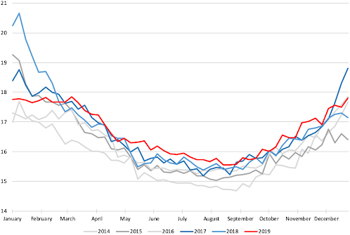
Figure 1 shows mortality rates per 100,000 in the U.S. week by week, taken separately for years from 2014 to 2019. We see strong similarity of the annual patterns with clear increase in the winter months. Year 2017 was known for especially deadly flu season, which is reflected in the curve of 2017 ending up high and the curve of 2018 starting up very high on the graph.

Figure 1.

U.S. weekly mortality in 2014–2019 (rate per 100,000).

To better illustrate our point, consistently with (Leavitt, 2021), we will adjust the numbers to the growing U.S. population using mortality rates rather than counts, and defining weekly excess mortality rate for week t=1,…,52 of the year s=2014,2015,…⁢2020 as the ratio

where mortality rate is defined as R⁢(t,s)=D⁢(t,s)/P⁢(s), where D⁢(t,s) is the death count, and P⁢(s) is adjusted mid-year population. The baseline mortality rate ∑u=20142018R⁢(t,u) is calculated as the average for non-perturbed (pre-COVID years).

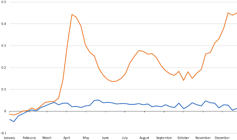
Figure 2 shows the values of 𝐸𝑀𝑅⁢(t,2019) in blue and 𝐸𝑀𝑅⁢(t,2020) in red. It is clear that while the graphs for 2019 and 2020 look very similar from January to March, year 2020 has seen dramatic increase of mortality for the remaining nine months. However, excess mortality in 2019 also stays above the average for most of the year. It is also interesting to observe higher variability of weekly data towards the end of 2019.

Figure 2.

U.S. weekly EMR, 2019 (blue) and 2020 (red).

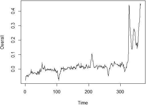
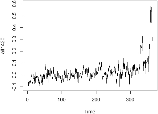
In order to analyze this effect further, we will look at the combined time series of excess mortality for 364 consecutive weeks 𝐸𝑀𝑅⁢(t,2014),…,𝐸𝑀𝑅⁢(t,2020) in Fig. 3. Applying ADF test for unit root and KPSS stationarity test, we observe evident lack of stationarity. It looks like there may exist a structural break between pre-COVID and COVID periods. We will try to identify the timing of this break and then further analyze pre-COVID and COVID time series separately.

Figure 3.

U.S. weekly EMR, from 2014 through 2020.

4.1ARIMA model for U.S. excess mortality rate

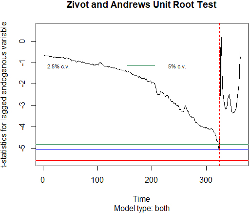
As it is suggested by Fig. 3, we will apply Zivot-Andrews structural break unit root test (Zivot & Andrews, 1992), and then suggest two possibly different time series models describing two periods: before and after the break. Zivot-Andrews test suggests a potential break at week 324 corresponding to the end of March 2020. It confirms the general timing of the pandemic onset in the U.S.

Figure 4.

Zivot-Andrews test results for weekly EMR, 2014-2020.

The next step is to build ARIMA models for the first 324 weeks starting in 2014 (pre-COVID period) and the last 40 weeks of 2020 (COVID period). As demonstrated by ADF unit root test rejected with p<0.01 and KPSS stationarity test not rejected with p>0.1, the pre-COVID time series may be considered stationary. Analysis of residual ACF, PACF and Box-Ljung-Pierce tests suggest the model ARIMA (2, 0, 0).

On the contrary, COVID time series (it is much shorter, so statistical conclusions may be less decisive) may be considered stationary by KPSS test with p>0.1, but ADF with p=0.557 test suggests existence of a unit root. Comparing ARIMA (1, 0, 0) and ARIMA (1, 1, 0) models from residual analysis point of view, we can make conclusion in favor of ARIMA (1, 1, 0). Higher p-values of Box-Ljung test suggest the absence of residual correlation.

Table 1

Model comparison for the U.S. excess mortality pre-COVID and COVID

	a0	a1	a2	AIC	Box-Ljung
	(st.error)	(st.error)	(st.error)		p-value
pre-COVID
(324 weeks)
𝐴𝑅𝐼𝑀𝐴⁢(1,0,0)	0.003	0.918)		-1965	0.002
	(0.007)	(0.024)
𝐴𝑅𝐼𝑀𝐴⁢(2,0,0)	0.003	0.708	0.235	-1981	0.210
	(0.010)	(0.055)	(0.055)
COVID
(40 weeks)
𝐴𝑅𝐼𝑀𝐴⁢(1,0,0)	0.267	0.908		-124	0.23
	(0.066)	(0.069)
𝐴𝑅𝐼𝑀𝐴⁢(1,1,0)	0	0.638		-136	0.80
		(0.156)

Statistically significant results in parametric estimation are boldfaced in Table 1.

The following Table 2 shows the one-week to four-week ahead forecast of U.S. excess mortality using the first 20 weeks after the structural break in the end of March 2020 and further accumulated data: we use 20 weeks to forecast weeks 21–24, then 24 weeks to forecast weeks 25–28, etc.

Table 2

Excess mortality forecast in the 2020 after the stuctural break using ARIMA (1, 1, 0)

Week	Lower bound	Forecast	Upper bound	Actual actual	MAE	MAPE
21	0.17	0.25	0.33	0.26
22	0.07	0.24	0.41	0.25
23	0	0.23	0.50	0.21
24	0	0.23	0.60	0.19	0.02	10%
25	0.09	0.17	0.24	0.17
26	0	0.15	0.31	0.16
27	0	0.14	0.39	0.18
28	0	0.13	0.47	0.14	0.02	11%
29	0.03	0.11	0.18	0.18
30	0	0.08	0.23	0.15
31	0	0.06	0.30	0.18
32	0	0.04	0.37	0.19	0.10	59%
33	0.12	0.20	0.28	0.26
34	0.05	0.21	0.37	0.27
35	0	0.22	0.45	0.31
36	0	0.22	0.53	0.33	0.08	27%
37	0.26	0.34	0.42	0.38
38	0.20	0.35	0.51	0.45
39	0.13	0.36	0.58	0.44
40	0.06	0.36	0.66	0.45	0.08	18%

It is difficult to compare the forecast quality with other sources since our use of excess mortality rather than the number of deaths is not standard. However, prediction interval coverage for the period is 100% and MAPE values are reasonable with the exclusion of Summer weeks 29–32, when new COVID growth occured but was not predicted by the model. It is not unusual for ARIMA models to fall behind with prediction in presence of new effects though the models eventually adjust to incorporate these effects in future forecasts.

4.2ARIMA model for Minnesota excess mortality rate

Performing similar analysis for the state of Minnesota, we consider excess mortality rates obtained by the same methodology as we applied to the entire U.S. Analyzing the weekly time series for 364 weeks from the beginning of 2014 to the end of 2020, we observe clear loss of stationarity in the last year of observations. Applying the structural break test, we detect a break at week 328 (early April) with a second possible structural break at week 345 (October), corresponding to the second wave of COVID in the Midwest.

ADF and KPSS tests show that the first 328 weeks do not expose non-stationarity, and by information criteria and residual analysis we can suggest ARIMA (3, 0, 0) to describe the behavior of the time series. COVID time series containing 36 weeks of 2020 is much harder to model with the existing data, and we end up with a highly non-stationary model. This is the result of building an ARIMA model by the data from the early period of pandemic, when the growth in mortality is highly non-stationary and non-linear. That is why in the next section we consider a longer period of time, establishing more reliable mortality patterns for the epidemic. While we will not be able to effectively predict further peaks, parametric model for a longer observation period will incorporate more patterns from the past and will be able to provide reasonable short-term forecasts.

Figure 5.

Minnesota weekly EMR, from 2014 through 2020.

Our analysis of overall mortality data from 2014–2020 shows in Fig. 5 the expected large rise in mortality in 2020 compared to other years. Less expected, the data also shows some positive excess mortality in 2019, even when accounting for the seasonality of deaths using ARIMA. Higher excess deaths are seen in the US generally and in Minnesota specifically starting as early as the fall of 2019, while structural breaks suggesting a significant increase in mortality can be detected in March 2020 in the U.S. and in April 2020 in Minnesota. A study from the Centers for Disease Control and Prevention tested U.S. blood donor samples from December 2019–January 2020 and found samples positive for COVID-19 antibodies in every one of the nine states surveyed (Basavaraju et al., 2020). A follow-up study from the National Institute of Health “All of Us” study also found COVID-19 antibodies in a number of stored blood samples from early 2020, suggesting the presence of COVID-19 prior to first reports (Althoff et al., 2021). These studies align with other international studies which suggest that COVID-19 was spreading around the world before the first reports of spread in winter of 2020 (Du et al., 2020; Apolone et al., 2020). (Lopreite et al., 2021) analyzed twitter mentions of pneumonia throughout Europe in late 2019/early 2020. Increased number of tweets concerned about pneumonia were noticed, especially in areas that later turned out to be major COVID hot-spots. As suggested in (Roberts et al., 2021), first case of COVID-19 in China may have been circulating as early as October 2019. Data from other nations, including France and Russia, have shown an abnormally high number of cases of and deaths from non-specific pneumonia in the fall of 2019 (Deslandes et al., 2020). It is possible that this rise in excess deaths in fall 2019 may suggest that COVID was affecting U.S. mortality earlier than currently believed.

Table 3

Model comparison for Minnesota excess mortality pre-COVID and COVID

	a0	a1	a2	a3	AIC	Box-Ljung
	(st.error)	(st.error)	(st.error)	(st.error)		p-value
pre-COVID
(328 weeks)
𝐴𝑅𝐼𝑀𝐴⁢(3,0,0)	0.007	0.265	0.124	0.239	-1177	0.60
	(0.006)	(0.054)	(0.056)	(0.055)
COVID
(36 weeks)
𝐴𝑅𝐼𝑀𝐴⁢(2,2,0)	0	- 0.746	- 0.272		-65	0.17
	0	(0.162)	(0.163)

This analysis in Table 3 demonstrates that at the state level, the excess mortality at the pandemic stage is substantially non-stationary and exposes one or two structural breaks. Since early 2020, it became possible to address the causes of death and analyze the total number of COVID cases. Therefore the further analysis introduces new variables for more extensive period of time. After a rapid rise in early 2020, the pandemic developed in rising and falling waves which suggests a possibility to use the tools fit for stationary time series.

5.VAR model for Minnesota

Using entire dataset available from the onset of COVID-19 up to the summer of 2021 on weekly observations of new COVID cases, hospitalizations, and deaths in the state of Minnesota (total of 67 weeks), we build VAR models (5) with k=3 and different lag depth. Since we analyze new weekly cases, hospitalizations, and deaths, stationarity of the time series is more feasible than for total (accumulated) cases deaths as analyzed in (Sahai et al., 2020).

First, we apply the KPSS test to check stationarity of the time series, which is not rejected for any of the three individual series with high p-value (>0.1), since the hypothesis of stationarity, the choice of d=0 and model 𝑉𝐴𝑅⁢(p) appear reasonable. Then we proceed with the model selection, which in our case suggests the choice of lag p. When we apply ’vars’ package in R (Pfaff & Stiegler, 2018), the lags from 1 to 4 are recommended by different information criteria: SIC is the most conservative with p=1, HQC and TPE concur on p=2, while AIC suggests p=4, which is almost prohibitive in terms of model size. If we start with p=1, we obtain the following results of parametric estimation and diagnostic tests.

When we analyze the variable Y(3)=𝐷𝑒𝑎𝑡ℎ, we do not see any significance of the lagged values of Y(1)=𝐶𝑎𝑠𝑒𝑠 and of Y(2)=𝐻𝑜𝑠𝑝.

In Table 3, the adjusted R2=0.9247. Boldface indicates significance of the coefficient. However, when we analyze the other two variables as dependent, they demonstrate a more complicated association pattern.

In Table 4, the adjusted R2=0.8876. Boldface indicates significance of the coefficients, and we see that new cases along with a stable association with the last week’s cases, acquire a negative dependence on last week’s deaths.

In Table 5, the adjusted R2=0.9121. We can see that new hospitalizations along with the last week’s data are also negatively associated with the last week’s deaths. This negative association may be a result of a mis-specified model. However, the size of this effect is relatively minor if we take into account the overall number of new cases vs deaths. It can be attributed to changes of the relative share of the vulnerable population in the course of pandemic development. These tables support our hypothesis that three variables we are studying are closely associated, and data on all three of them might be helpful while predicting the short-term future behavior of any of the variables.

Multivariate ARCH Lagrange multiplier test does not detect any heteroscedascticity in the model and CUSUM test does not detect significant structural breaks. However, Jarque-Bera test as well as skewness and curtosis tests suggest the absence of normality which indicates that VAR (1) model might be too small and there are some factors which it does not address. Also, a portmanteau test built into ‘vars’ package, yields p-value of 0.026 for the null hypothesis of no serial residual correlation and hints at possible autocorrelations in the residuals, which suggests possibly a higher number of lags. The graphs of PACF for all three variables support this suggestion.

However, running VAR model with higher number of lags (e.g., p=2, as suggested by HQC and TPE) does not provide a better overall result and more accurate forecasts. Jarque-Bera test confirms normality of residuals and portmanteau test confirms the absence of residual correlation, which suggests that depth p=1 is sufficient (see Table 7).

The adjusted R2=0.9225. Boldface indicates significance of the coefficient. However, most of the coefficients of lag 2 in Table 6 are not statistically significant, which might be an indication of multicollinearity. It allows us to suspect overparameterization and, agreeing with SIC, recommend the more parsimonious choice of p=1, which we will adopt in the sequel. It would be more intuitive to establish statistical relationships of Deaths time series with lagged values of hospitalizations and cases, however the model shows that a more reliable association is established with lagged Deaths, which is an evidence of strong autocorrelation in this series.

6.Comparison of VAR models for states

Minnesota and Wisconsin are two adjacent midwestern states sharing the border on the St. Croix river. Geographical and demograhic situation of the states is similar: both states have substantial rural populations along with some high-populated metro areas.

In summer of 2020, the state of Minnesota introduced a comprehensive program of social distancing measures including mandatory use of masks indoors, restriction of social gatherings both indoors and outdoors, closing and restricting activity of government public services, fitness facilities, bars and restaurants. In the meantime, restrictions in Wisconsin were much weaker, with fitness clubs and bars open without restrictions for most of the summer.

We will use the daily and weekly counts of COVID cases, hospitalizations and deaths obtained from state public health databases (MN Dept of Health, 2021; WI Dept of Health Services, 2021) to model the COVID development in Minnesota and Wisconsin, and also, for the sake of comparison, in such geographically distant states as Colrado (CO Dept of Public Health and Environment, 2021) and Georgia (GA Dept of Hublic Health and Environment, 2021). We will look for similarities and differences of COVID epidemic development in these four states.

The objective is to build VAR models for COVID-19 development in different states and compare the parametric values, analyzing possible sources of discrepancies. Colorado and Georgia were included for comparison to represent differing COVID measures and actions in different regions of the country. Colorado has high tourism and travel rates, which potentially augmented COVID spread and COVID cases and deaths. Georgia and the US South had lower vaccination rates as well as higher COVID transmission likely due to lack of comprehensive measures.

Minnesota, Wisconsin, Georgia, Colorado state differences in COVID rates could reflect differences in population density (MN: 70.5 residents per square mile, WI: 107.3 residents per square mile, GA: 149 residents per square mile, CO: 59 residents per square mile), timing and severity of stay-at-home orders and closures, mask mandates, extent of school distance learning, travel in and out of state, etc.

We will concentrate on the mortality with 𝐷𝑒𝑎𝑡ℎ𝑠t being the principal dependent variable. First, let us look at the weekly mortality data for four states in question. It looks like both Minnesota and Colorado demonstrate two distinct mortality peaks coresponding to two waves of the disease corresponding to the first and the second half of 2020. From Table 8 we see In case of Wisconsin, the first peak is less expressed and the second is wider, beginning earlier and ending up later. Georgia demonstrates a more complicated pattern, with additionasl peaks in Summer 2020 and delayed rise of mortality in early 2021. One should also pay attention to the difference in the vertical scale for Georgia graph, exposing a higher overall mortality or relative populations of states.

Figure 6.

Weekly COVID mortality in Minnesota.

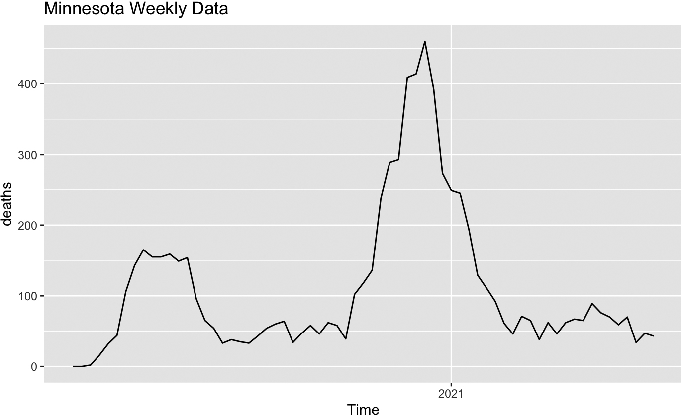
Figure 7.

Weekly COVID mortality in Colorado.

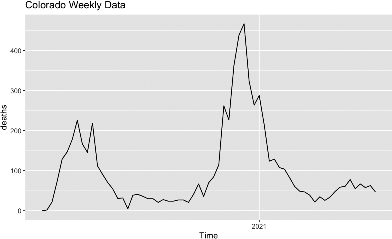
The next step of analysis will allow us to see how the patterns visualized on the graphs reveal themselves in VAR (1) models suggested for different states. Similar to the case of Minnesota discussed in Scetion 5, model selection for the other states also suggests restricting our attention to lag p=1. We will be able to provide some pairwise comparisons. For that purpose, let us list in one table the coefficients for all three lag 1 variables with two-standard error intervals. The boldfaced values correspond to non-overlapping intervals or coefficients for other states, which are statistically significantly different from those for Minnesota.

Figure 8.

Weekly COVID mortality in Wisconsin.

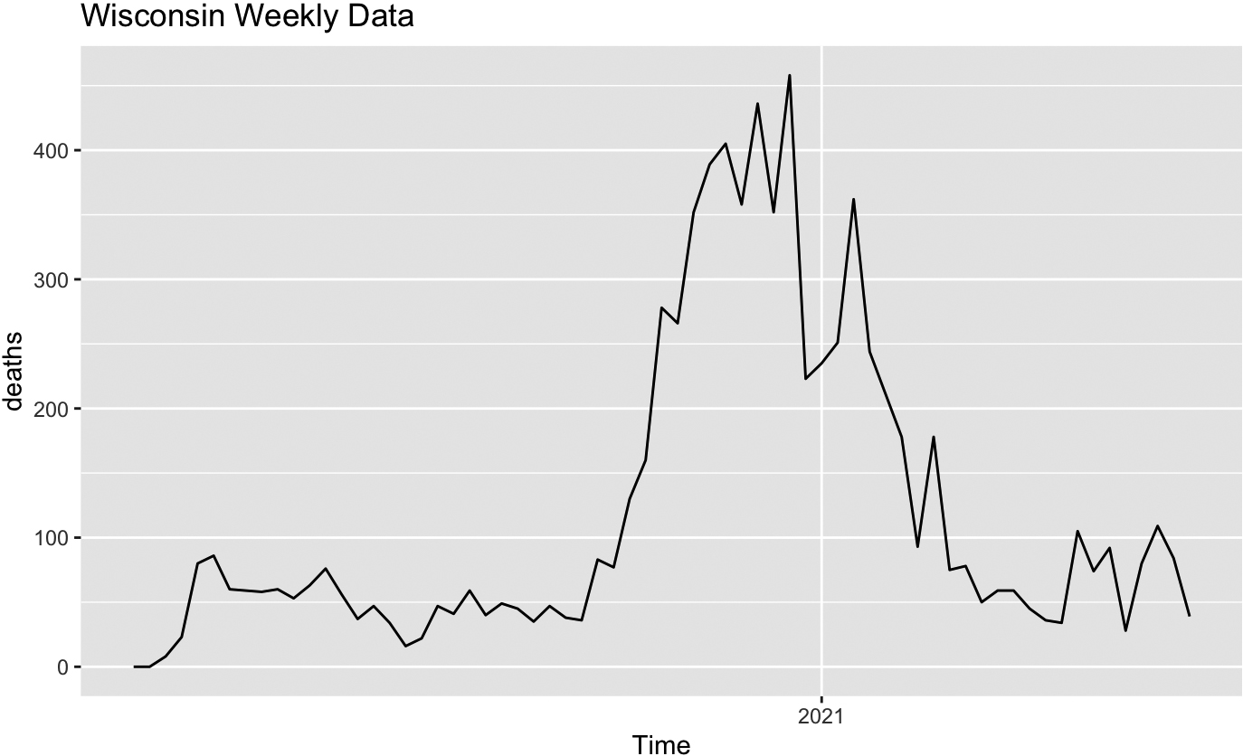
Figure 9.

Weekly COVID mortality in Georgia.

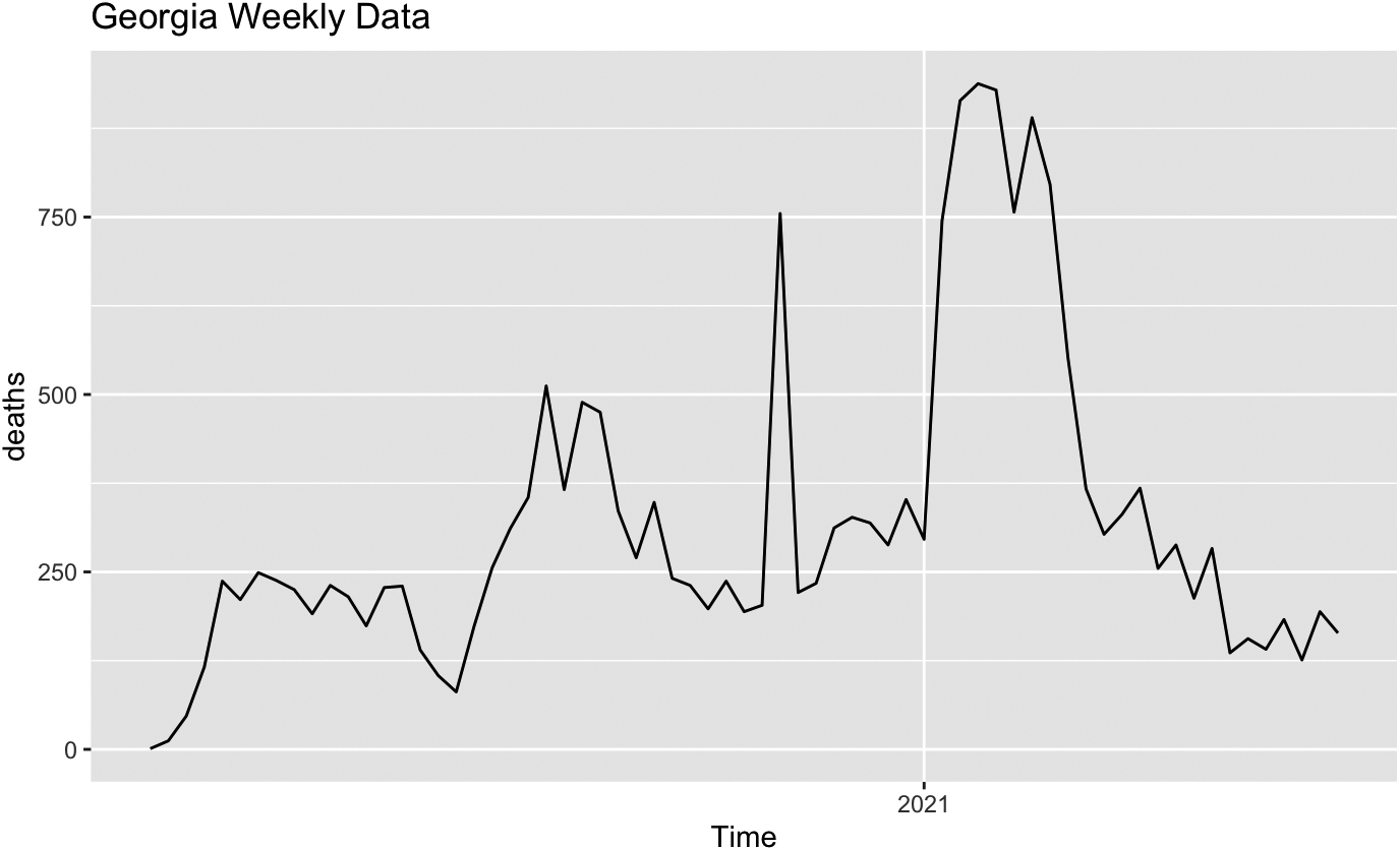
From Table 7 we see that, while Colorado and Minnesota provide quite similar VAR (1) models, where the previous week’s death count is sufficient to predict the next week’s count, the model for Wisconsin also suggests that knowledge of previous week’s hospitalizations is also helpful for death forecast, and the model for Georgia suggests that the previous week’s case count might matter.

Comparison of COVID cases, hospitalizations and deaths in four states based on VAR models may be based on estimated model parameters for different states. This analysis does not allow for a definitive conclusion whether geographical differences and/or the distinctly different approach to preventive quarantine measures brings about different patterns of epidemics development. Models for Minnesota and Colorado look simiar while models for Minnesota and Wisconsin are somewhat different, with Wisconsin showing a wider first peak and a later secondary peak of infections. Georgia looks different from the other three, with a much later peak in cases. All these features are reflected in the difference of model parameters. This comparison cannot be used to justify any further conclusions related to the efficiency of the quarantine measures since there are other factors to be taken into account, there is no rigid boundary between the states, and interstate travel was not restricted in any way.

7.Vaccination and VAR forecast

The standard out-of-sample validation approach suggests that we can use part of the data for model construction and the rest of the data for model validation, when we compare forecasted and actual values of the dependent variables. To illustrate the short-term predictive quality of VAR models with or without external effects, we will use the example of COVID-related deaths in Minnesota observed for 67 weeks from March 2020 to June 2021. Out-of-sample forecast for weeks 52–55 is based on the model parameters estimated by the first 51 observations, weeks 56–59 based on the first 55 observations, etc. A four-week window is recommended in (Bilinski & Salomon, 2021) and other related analyses.

Numerical values for four-week out-of-sample forecast (with 95% prediction intervals) based on previous observations are compared to actual values in Table 9 in the following table. Four-week periods are separated by horizontal lines. Asterisks correspond to the cases when actual values did not fit into 95% prediction intervals. They appear in the third four-week period analyzed (weeks 60–63: April/May 2021). This is the period following the most active vaccination of elderly population in Minnesota.

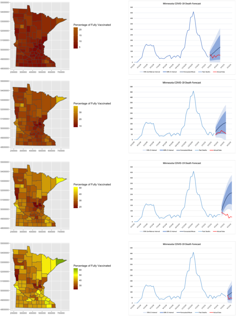
Figure 10.

Forecast based on VAR models.

Overall, MAE and MAPE values are high, but not out of line with the predictions discussed in (Johansson et al., 2020). Coverage by confidence intervals is 87.5%. Parametric estimation and forecasting was also carried out for VAR (2) and VAR (4), but the forecast errors are even larger for these.

In order to provide a graphical insight, four horizontal panels of Fig. 10 demonstrate performance of the models based on pre-vaccination periods ending in March and April 2021, vaccination period ending in May 2021, and post-vaccination period ending in June 2021, when they are used for short-term (four-week) forecast.

Left sub-panels reflect the vaccination maps measuring accumulated percentages of fully vaccinated by county in the end of the each of four months (February through May). Right sub-panels depict actual data on COVID-related deaths, followed for illustrative purposes by the eight-week out-of-sample forecast. Solid blue lines correspond to predicted deaths, with dark blue and light blue bands corresponding to 90% and 95% prediction intervals. The red lines show actual deaths.

Pre-vaccination (February and March) models behave reasonably well, with actual data within prediction intervals, while the peak vaccination (April/May) model’s forecast substantially overestimates the actual mortality. This difference between models built by different periods may be used to demonstrate the strong negative effect of vaccination on COVID-related mortality since the model predicts higher mortality without vaccination. It also shows that the model should be used with caution when new effects, such as vaccination or variants, are introduced. It is interesting that post-vaccination (May/June) model returns to feasible forecast accuracy since the past data include the vaccination period, and its effect is taken into account.

8.Conclusions

We suggest ARIMA models of excess deaths as a simple tool of addressing mortality at the early pandemic stages, using mortality history only without getting deep into specific epidemiological factors. These models are not going to provide full long-term picture, but may be helpful for short-term forecast. Structural breaks, bringing about non-stationarity and substantial growth in mortality are detected in March for the U.S., and in April and October for Minnesota.

In the present paper we do not compare excess mortality to official COVID mortality as reported by CDC.We analyze excess mortality at the early pandemic stages, when COVID-specific data are not available. At the later stages, we used COVID-specific data as provided by CDC and state healthcare systems.

VAR models built for Minnesota suggest that the past experience of COVID cases, hospitalizations and deaths studied in their interdependence can provide valuable modeling information for the later pandemic stages. The advantage of vector autoregressive time series modeling is in avoiding the use of external pandemic factors which might be unclear or controversial. Comparison of four different states suggests both similarities and differences in COVID-19 development, which may help to address local public health policy decisions.

Out-of-sample validation of VAR models of COVID-related deaths in Minnesota provided satisfactory results with the exclusion of the peak vaccination period when actual mortality was overestimated by the model built by pre-vaccination data. This may serve as an indirect confirmation of the efficiency of vaccination in slowing down the disease-related mortality, compare (Moghadas et al., 2021).

Finally, one of the objectives is to introduce low-dimensional vector autoregresion (VAR) technique to an actuarial mortality study. VAR is widely used in such fields as econometrics, but it is less popular in eplidemiology, and even less so in actuarial mortality modeling. Our conclusion is that low-dimensional VAR may serve as an efficient tool in presence of several related variables (such as cases, hospitalizations and deaths) observed on a regular basis and having a structure of a vector time series. Our short-term (four-week) predictions based on VAR implementation were effective as demonstrated by out-of-sample validation, confirming conclusions of (Bilinski & Salomon, 2021).

Once sufficient time passes, there will be a need to use the most recent CDC “corrected data” (notably, the CDC periodically revises datasets) to refine this paper with updated deaths and include the added adjustments referred to in the earlier sections. Our predictive model professes to be useful in making short-term best estimate projections of deaths, in conjunction with ARIMA, VAR and the actuarial techniques outlined herein.

References

[1] | Adiga, A., Dubhashi, D., Lewis, B., et al. ((2020) ). Mathematical models for COVID-19 pandemic: A comparative analysis. J Indian Inst Sci, 100: , 793-807. doi: 10.1007/s41745-020-00200-6. |
[2] | Akaike, H. ((1974) ). A new look at the statistical model identification. IEEE Transactions on Automatic Control, 19: (6), 716-723. |
[3] | Althoff, K.N., Schlueter, D.J., Anton-Culver, H., et al. ((2021) ). Antibodies to SARS-CoV-2 in All of Us Research Program Participants, January 2–March 18, 2020, Clinical Infectious Diseases, ciab519. doi: 10.1093/cid/ciab519. |
[4] | Antulov-Fantulin, N., & Böttcher, L. ((2022) ). On the accuracy of short-term COVID-19 fatality forecasts. BMC Infect. Dis., 22: , 251. doi: 10.1186/s12879-022-07205-9. |
[5] | Apolone, G., Montomoli, E., Manenti, A., et al. (Nov (2020) ). Unexpected detection of SARS-CoV-2 antibodies in the prepandemic period in Italy. Tumori, 11: : 300891620974755. doi: 10.1177/0300891620974755. Epub ahead of print. PMID: 33176598. |
[6] | Basavaraju, S.V., Patton, M.E., Grimm, K., et al. (15 June (2021) ). Serologic Testing of US Blood Donations to Identify Severe Acute Respiratory Syndrome Coronavirus 2 (SARS-CoV-2) – Reactive Antibodies. December 2019–January 2020, Clinical Infectious Diseases, V. 72–12, e1004-E1009. doi: 10.1093/cid/ciaa1785. |
[7] | Bellhouse, D.R., & Panjer, H.H. ((1981) ). Stochastic Modeling of Interest Rates with Applications to Life Contingencies. The Journal of Risk and Insurance, part I: 47(1), 91-110; part II: 48(4), 628-637. |
[8] | Bhattacharyya, A., Chakraborty, T., & Rai, S.N. ((2022) ). Stochastic forecasting of COVID-19 daily new cases across countries with a novel hybrid time series model. Nonlinear Dyn, Jan 13, 1-16. doi: 10.1007/s11071-021-07099-3. PMID: 35039713; PMCID: PMC8754528. |
[9] | Bilinski, A., & Salomon, J.A. ((2021) ). Pandemic Models Can Be More Useful: Here’s How, Health Affaris Forefront, 202110.1377/forefront.20210831.560758. |
[10] | Box, G.E.P. ((2015) ). Time Series Analysis: Forecasting and Control, Wiley, ISBN 978-1-118-67502-1. |
[11] | Box, G.E.P., & Jenkins, G. ((1970) ). Time Series Analysis Forecasting and Control, Published by (HD), SF CA USA, ISBN 10: 1619605848ISBN 13: 9781619605848 |
[12] | CDC COVID-19 Forecasts: Death. ((2022) ). Reported and forecasted new and total COVID-19 deaths as of May 9, 2022. https://www.cdc.gov/coronavirus/2019-ncov/science/forecasting/forecasting-us.html. |
[13] | CDC Wonder. ((2021) ). Available online https://wonder.cdc.gov/ucd-icd10.html (accessed December 17, 2021). |
[14] | Chitwood, M.H., Russi, M., Gunasekera, K., Havumaki, J., Pitzer, V.E., Salomon, J.A., Swartwood, N., Warren, J.N., Weinberger, D.M., Cohen, T., & Menzies, N.A. ((2020) ). Reconstructing the course of the COVID-19 epidemic over 2020 for US states and counties: results of a Bayesian evidence synthesis model. doi: 10.1101/2020.06.17.20133983. |
[15] | Colorado Department of Public Health and Environment. ((2021) ). Available online https://covid19.colorado.gov/data (accessed December 17, 2021). |
[16] | Conde-Gutiérrez, R.A., Colorado, D., & Hernández-Bautista, S.L. ((2021) ). Comparison of an artificial neural network and Gompertz model for predicting the dynamics of deaths from COVID-19 in México. Nonlinear Dyn., 104: (4), 4655-4669. doi: 10.1007/s11071-021-06471-7. Epub 2021 Apr 30. PMID: 33967393. |
[17] | Deslandes, A., Berti, V., Tandjaoui-Lambotte, Y., Chakib, A., Carbonnelle, E., Zahar, J.R., Brichler, S., & Cohen, Y. ((2020) Jun). SARS-CoV-2 was already spreading in France in late December 2019. Int J Antimicrob Agents, 55: (6), 106006. doi: 10.1016/j.ijantimicag.2020.106006. |
[18] | Doornik, J.A., Castle, J.L., & Hendry, D.F. ((2022) ). Short-term forecasting of the coronavirus pandemic. International Journal of Forecasting, 38: (2), 453-466. ISSN 0169-2070, doi: 10.1016/j.ijforecast.2020.09.003. |
[19] | Du, Z., Javan, E., Nugent, C., Cowling, B.J., & Meyers, L.A. ((2020) Sep). Using the COVID-19 to influenza ratio to estimate early pandemic spread in Wuhan, China and Seattle, US. EClinicalMedicine, 26: , 100479. doi: 10.1016/j.eclinm.2020.100479. Epub 2020 Aug 12. PMID: 32838239; PMCID: PMC7422814. |
[20] | Georgia Department of Public Health. ((2021) ). Available online https://dph.georgia.gov/covid-19-daily-status-report (accessed December 17, 2021). |
[21] | Guibert, Q., Lopez, O., & Piette, P. ((2019) ). Forecasting mortality rate improvements with a high-dimensional VAR. Insurance: Mathematics and Economics, 88: , 255-72. |
[22] | Hamilton, J. ((1994) ). Time Series Analysis, Princeton University Press, ISBN 9780691042893. |
[23] | Hannan, E.J., & Quinn, B.G. ((1996) ). The Determination of the order of an autoregression. Journal of the Royal Statistical Society, Series B, 41: , 190-195. |
[24] | Imperial College COVID Response Team. ((2022) ). Short-term forecasts of COVID-19 deaths in multiple countries. May 2022. https://mrc-ide.github.io/covid19-short-term-forecasts/. |
[25] | Johansen, S. ((1996) ). Likelihood Based Inference in Conitegrated Vector Autoregression Models, Oxford University Press, Oxford. |
[26] | Johansson, M.A., Reich, N.G., et al. ((2020) ). Ensemble Forecasts of Coronavirus Disease 2019 (COVID-19) in the U.S. doi: 10.1101/2020.08.19.20177493. |
[27] | Kotze, K. ((2020) ). Tutorial: Vector Autoregession Models, http://kevinkotze.github.io/ts-7-tut. |
[28] | Kremer, E. ((2005) ). The correlated chain-ladder method for reserving in case of correlated claims developments. Blätter DGVFM, 27: , 315-322. doi: 10.1007/BF02808313. |
[29] | Leavitt, R. 2021. (2020). Excess Deaths in the U.S. General Population by Age and Sex, Mortality and Logevity, 2021, February, Society of Actuaries. |
[30] | Lee, R.D., & Carter, L.R. ((1992) ). Modeling and Forecasting U.S. Mortality. Journal of the American Statistical Association, 87: (419). |
[31] | Li, H., & Shi, Y. ((2021) ). Mortality Forecasting with an Age-Coherent Sparse VAR Model. Risks, 9: , 35. doi: 10.3390/risks9020035. |
[32] | Lopreite, M., Panzarasa, P., Puliga, M., et al. ((2021) ). Early warnings of COVID-19 outbreaks across Europe from social media. Sci Rep, 11: , 2147. doi: 10.1038/s41598-021-81333-1. |
[33] | Lütkepohl, H. ((2006) ). New Introduction to Multiple Time Series Analysis, Springer, New York. |
[34] | Minnesota Department of Health. ((2021) ). Available online https://www.health.state.mn.us/diseases/coronavirus (accessed December 17, 2021). |
[35] | Moghadas, S.M., Sah, P., Fitzpatrick, M.C., Shoukat, A., Pandey, A., Vilches, T.N., Singer, B.H., Schneider, E.C., & Galiani, A.P. ((2021) ). COVID-19 deaths and hospitalizations averted by rapid vaccination rollout in the United States. doi: 10.1101/2021.07.07.21260156. |
[36] | Mukhaiyar, U., Widyanti, D., & Vantika, S. ((2021) ). The time series regression analysis in evaluating the economic impact of COVID-19 cases in Indonesia, Model Assisted Statistics and Applications, 16: (3), 197-210. |
[37] | Musawa, N., & Mwaanga, C. ((2017) ). The Impact of Pension Funds’ Investments on the Capital Market – The Case of Lusaka Securities Exchange. American Journal of Industrial and Business Management, 7: , 1120-1127. doi: 10.4236/ajibm.2017.710080. |
[38] | Oliveira, T.P., & Moral, R.A. ((2021) ). Global short-term forecasting of COVID-19 cases. Sci Rep, 11: , 7555. doi: 10.1038/s41598-021-87230-x. |
[39] | Park, C., Kim, D.-S., & Lee, K.Y. ((2022) ). Asset allocation efficiency from dynamic and static strategies in underfunded pension funds, Journal of Derivatives and Quantitative Studies. doi: 10.1108/JDQS-10-2021-0025. |
[40] | Pfaff, B., & Stigler, M. ((2018) ). Package ‘vars’. http://www.pfaffikus.de. |
[41] | Piazzola, C., Tamellini, L., & Tempone, R. ((2021) ). A note on tools for prediction under uncertainty and identifiability of SIR-like dynamical systems for epidemiology, Mathematical Biosciences, 332, February 2021. doi: 10.1016/j.mbs.2020.108514. |
[42] | Roberts, D.L., Rossman, J.S., & Jarić, I. ((2021) ). Dating first cases of COVID-19. PLOS Pathogens, 17: (6), e1009620. doi: 10.1371/journal.ppat.1009620. |
[43] | Rosenfeld, R., & Tibshirani, R.J. ((2021) ). Epidemic tracking and forecasting: Lessons learned from a tumultuous year. PNAS, 118: , 51. doi: 10.1073/pnas.2111456118. |
[44] | Sahai, A.K., Rath, N., Sood, V., & Singh, M.P. ((2020) ). ARIMA modelling and forecasting of COVID-19 in top five affected countries. Diabetes Metab. Syndr., 14: (5), 1419-1427. doi: 10.1016/j.dsx.2020.07.042. Epub 2020 Jul 28. PMID: 32755845. |
[45] | Schwarz, G.E. ((1978) ). Estimating the dimension of a model. Annals of Statistics, 6: (2), 461-464. doi: 10.1214/aos/1176344136. |
[46] | Sims, C. ((1980) ). Macroeconomics and reality. Econometrica, 48: (1), 1-48. doi: 10.2307/1912017. JSTOR 1912017. |
[47] | Watier, L., & Richardson, S. ((1995) ). Modelling of an epidemiological time series by a threshold autoregressive model. The Statistician, 44: (3), 353-364. |
[48] | Weinberger, D.M., Chen, J., Cohen, T., et al. ((2020) ). Estimation of Excess Deaths Associated With the COVID-19 Pandemic in the United States, March to May 2020. JAMA Intern Med., published online July 01, 2020. doi: 10.1001/jamainternmed.2020.3391. |
[49] | Wisconsin Dept of Public Services. ((2021) ). Available online https://www.dhs.wisconsin.gov/covid-19/index.htm (accessed December 17, 2021). |
[50] | Zivot, E., & Andrews, D.W.K. ((1992) ). Further evidence on the great crash, the oil-price shock, and the unit-root hypothesis. Journal of Business and Economic Statistics, 10: (3), 251-270. doi: 10.2307/1391541. |