
Nonparametric modeling of multiple decrements subject to dependent censoring and masking
Abstract
In this paper we develop self-consistent and smoothed dependent estimators for the cause-specific failure time density in a competing risks context, employed in the presence of both left-censored and right-censored data, while allowing for masking of the failure cause. Dependence will be incorporated between the failure times and both the censoring times and the masked causes with the use of both Kernel Regression and Multivariate Multiple Regression at each iteration of the algorithm. Our approach to modeling the cause-specific failure times is intended to be the most automated and data-driven approach possible.
1.Introduction
The theory of competing risks is employed by statisticians, actuaries (multiple decrement theory), engineers (reliability theory), demographers, biologists, and others. Scientists from these various disciplines who are involved in the modeling of time-to-event data with competing modes of failure will very likely encounter censored and/or masked data, as well as statistical dependence issues, in their work. This present work addresses a significant void in the literature by providing a nonparametric framework for modeling competing risks data while simultaneously allowing for the possibility of censoring, masking, and the statistical dependence of these latter phenomena with the failure times themselves. The doubly-censored and nonparametric SC-CR Algorithm of Adamic (2010) will be utilized as the engine to generate the cumulative incidence probabilities. However, the SC-CR Algorithm will be enhanced at each iteration by employing either Kernel Regression or Multivariate Multiple Regression (MMR) to account for the dependence between the censoring times and the masked failure causes with the failure time distribution, but in such a manner so as to maintain the statistical attribute of self-consistency for the resulting estimators. For illustrative purposes, the proposed models will be applied to a bivariate Trypanosomiasis data set.
This research fits in well within the overall trajectory of scholarship that has taken shape in the niche area of nonparametric competing risks research. Nonparametric maximum likelihood estimators (NPMLEs) of the cumulative incidence for competing risks data were pioneered by Aalen (1976) and Kalbfleisch and Prentice (1980). Subsequently, Dinse (1982) proposed an NPMLE for right-censored and masked competing risks data to be computed with the explicit use of a Dempster et al. (1977) Expectation-Maximization (EM) algorithm. Hudgens et al. (2001) first presented an NPMLE estimated using an EM algorithm for competing risks data, subject to both interval-censoring and truncation. Jewell et al. (2003) and Groeneboom et al. (2008) follow this trajectory with similar studies of nonparametric maximum likelihood estimators for current status data. More recently, Adamic (2010), Adamic et al. (2010), and Adamic and Guse (2016) developed generalizations of Turnbull’s (1974, 1976) classical univariate algorithms for modeling competing risks. These models, based on Turnbull’s self-consistent algorithm, can be shown to be species of EM algorithms. Overall, distribution-free models that can be employed in a multiple decrement context have received relatively little attention to date, in part due to the complexity that censoring and masking carry in their respective trains. Our research is geared towards developing models that are as automated as possible, by keeping the number of assumptions to an absolute minimum – and this aim is actualized in the present work.
2.The SC-CR Algorithm for doubly-censored data
The first portion of Section 2, which summarizes the SC-CR Algorithm for doubly-censored data, is predominantly from Adamic (2010) and/or Adamic et al. (2010) and can be implemented as follows. The steps, statements, and logic of the algorithm will be directly generalized from those of the single variable algorithm of the standard textbook by Klein & Moeschberger (1997).
2.1The SC-CR algorithm for doubly-censored data
Step 0: Provide initial estimates of the overall survival probabilities at each
Step 1: Using the current estimates of
(1)
Step 2: Using the results of the previous step, estimate the number of cause-specific failures at time
(2)
Step 3: Compute
(3)
jointly for all of the time points
Partial masking can be introduced into the algorithm. For details, consult Adamic and Guse (2016). In terms of self-consistency, Adamic (2010) outlines a proof that the SC-CR Algorithms (for both the partially masked and completely masked cases) produce self-consistent estimators of the CIF’s for each failure mode. Although we strongly suspect that the CIF’s derived from the SC-CR Algorithms are also NPMLE’s, we will be content to rely on the statistical merits of self-consistency for the present work.
Despite the novelty of modeling masked competing risks data using an EM-type algorithm, there is a significant drawback associated with the various approaches that have been developed to date. As opined in Hudgens et al. (2001), estimators of this type will have the unwelcome property that the resulting estimators of the survival distribution will be undefined over a potentially large set of regions. Indeed, the problem is even more acute in the multiple-decrement environment: the SC-CR Algorithms of Adamic (2010) and Adamic and Guse (2016) can be seen to converge only over a class of intervals that were dubbed cause-specific innermost intervals. To remedy this problem, we have chosen to generalize a univariate kernel density estimator found in Braun et al. (2005) that was used to fill in the gaps between the univariate innermost intervals that were created by invoking the self-consistent EM algorithm of Turnbull (1976). The converged estimator of the failure rate distribution is often difficult to smooth, due to the large gaps often exhibited between innermost intervals, as well as the attendant multi-modal dispersion of the probability distribution that will typically arise when there are many gaps between the probability masses. As mentioned in Duchesne and Stafford (2001), adopting a kernel smoothed estimator at each iteration avoids the bias created by arbitrarily assigning probability mass at the right end points of the innermost intervals, as is also recommended by Pan (2000), and is furthermore better at borrowing more information from neighboring data points than would otherwise be the case. Duchesne and Stafford (2001) go on to state that since the innermost intervals are effectively no longer present, the kernel modification moves the algorithm away from problem causing areas – areas where Turnbull’s algorithm can sometimes get stuck at local solutions (also see Li et al., 1997, for further details on this point).
3.Kernel Regression modification to the SC-CR Algorithm
For motivation, let us first assume the survival data are interval-censored. Stafford (2005), drawing on the work of Goutis (1997), argues that a natural extension of the standard kernel smoothing weight is to define
(4)
the kernel density estimate of
(5)
for a fixed kernel function
The function npreg, part of the nonparametric np Package in R, is used to execute the Kernel Regression, an approach based on Li and Racine (2003), Li and Racine (2004), and Racine and Li (2004). The function utilizes data-driven (sometimes referred to as automated) bandwidth selection methods. As noted by Li and Racine (2003), traditional nonparametric kernel methods presume that the underlying data is continuous in nature, which is frequently not the case (and is not the case in the way we are regressing on censored and masked data, which are indicator based, and hence categorical), and so they develop their methodology using what they call generalized product kernels. Further details regarding the npreg function can easily be found online in the R documentation for the np Package.
Using a kernel smoothing mechanism at each iteration of the SC-CR Algorithm, the density estimate at the
(6)
conditioning on all observations,
(7)
where it is understood that the estimator is derived from the particulars of the chosen Kernel Regression routine. The span,
The following theorem shows that as the bandwidth tends to zero, the smoothed estimator of the CIF approaches the self-consistent CIF. The theorem statement, steps, and logic of the proof are direct generalizations of an analogous univariate proof from Braun et al. (2005).
.
Let
(8)
Proof: The self-consistent CIF is,
(9)
(10)
since
(11)
The kernel weight function is also a valid PDF that approaches the empirical distribution, and so,
(12)
(13)
since
(14)
(15)
(16)
4.MMR modification to the SC-CR Algorithm
The multivariate linear regression model is
(17)
where
(18)
with
(19)
or, summarily,
(20)
Using least squares estimates
(21)
(22)
The orthogonality present among the residuals, predicted values, and columns of
The foregoing was felicitous, as we want to explicitly maintain the statistical attribute of self-consistency when adding the dependent smoothing at each iteration of the SC-CR Algorithm. A proof to this effect is as follows.
4.1Proof for the self-consistency of the MMR estimators
Generalizing and adapting the preceding notation, the MMR estimator at a failure time
By keeping track of the censoring and masking types at each time point, we can construct indicator (or categorical, as necessary) regressors just like we did for Kernel Regression. We can run the modified SC-CR Algorithm just as before, only this time, using MMR regression at each iteration.
5.Application to a data set
The Trypanosoma brucei is a parasite that causes the rare disease African trypanosomiasis, colloquially referred to as African sleeping sickness. There are two forms that the disease can assume: the neurological form (N) and the lymphatic-sanguine (LS) form. These will comprise the two competing modes of failure, where the failure time,
Table 1
Summary of the trypanosomiasis data
| Case | Year | Age at infection | Form of disease |
|---|---|---|---|
| 1 | 1980 | [20,20] | N |
| 2 | 1981 | (0,29] | LS |
| 3 | 1981 | [29,29] | LS |
| 4 | 1981 | (0,32] | LS |
| 5 | 1981 | [43,43] | N |
| 6 | 1982 | (0,19] | LS |
| 7 | 1982 | [23,23] | N |
| 8 | 1983 | (0,40] | LS or N |
| 9 | 1984 | [24,24] | N |
| 10 | 1984 | (0,31] | N |
| 11 | 1986 | [13,13] | N |
| 12 | 1988 | [2,2] | N |
| 13 | 1988 | (0,34] | N |
| 14 | 1990 | [27,27] | N |
| 15 | 1991 | [34,34] | N |
| 16 | 1992 | (0,62] | LS or N |
| 17 | 1992 | (0,50] | N |
| 18 | 1993 | (0,30] | N |
| 19 | 1993 | [27,27] | LS |
| 20 | 1993 | [30,30] | N |
| 21 | 1996 | [53,53] | N |
| 22 | 1997 | (0,53] | LS |
| 23 | 1998 | [45,45] | LS |
| 24 | 1999 | (0,50] | LS |
| 25 | 1999 | (0,34] | LS or N |
| 26 | 2001 | [28,28] | N |
The SC-CR Algorithm was applied to the data. The raw results are given in the first and second columns of Table 2 under the subheading, “Unsmoothed”. As can be gleaned from the abundance of zeros, there is the conspicuous presence of many gaps between the cause-specific innermost intervals. Therefore, the use of Kernel Regression smoothing is especially opportune. The first Kernel Regression used only the masking information for creating the regressors, not the censoring. Masking regressors (or covariates) can easily be created by assigned an indicator of 1 or 0, if a specific cause (in this case, cause N or LS) was possible at each failure time point in the data set. The npreg Kernel Regression routine was then executed at each iteration of the SC-CR Algorithm.
Table 2
Dependent kernel regression results
| Age | Unsmoothed | Dep masking | Dep censoring | Dep mask/cens | ||||
|---|---|---|---|---|---|---|---|---|
|
|
|
|
|
|
|
|
|
|
| 2 | 0.112 | 0.000 | 0.097 | 0.002 | 0.098 | 0.011 | 0.111 | 0.000 |
| 13 | 0.112 | 0.000 | 0.082 | 0.002 | 0.082 | 0.011 | 0.091 | 0.000 |
| 19 | 0.000 | 0.000 | 0.001 | 0.015 | 0.001 | 0.001 | 0.000 | 0.000 |
| 20 | 0.075 | 0.000 | 0.074 | 0.002 | 0.074 | 0.011 | 0.079 | 0.000 |
| 23 | 0.075 | 0.000 | 0.071 | 0.002 | 0.071 | 0.011 | 0.077 | 0.000 |
| 24 | 0.075 | 0.000 | 0.070 | 0.002 | 0.070 | 0.011 | 0.077 | 0.000 |
| 27 | 0.075 | 0.075 | 0.067 | 0.015 | 0.076 | 0.041 | 0.075 | 0.075 |
| 28 | 0.075 | 0.000 | 0.065 | 0.002 | 0.065 | 0.011 | 0.076 | 0.000 |
| 29 | 0.000 | 0.075 | 0.001 | 0.038 | 0.057 | 0.011 | 0.000 | 0.075 |
| 30 | 0.068 | 0.000 | 0.072 | 0.002 | 0.056 | 0.011 | 0.068 | 0.000 |
| 31 | 0.000 | 0.000 | 0.062 | 0.002 | 0.000 | 0.001 | 0.000 | 0.000 |
| 32 | 0.000 | 0.000 | 0.001 | 0.015 | 0.000 | 0.001 | 0.000 | 0.000 |
| 34 | 0.054 | 0.000 | 0.056 | 0.002 | 0.051 | 0.011 | 0.055 | 0.000 |
| 40 | 0.000 | 0.000 | 0.000 | 0.002 | 0.000 | 0.001 | 0.000 | 0.000 |
| 43 | 0.046 | 0.000 | 0.041 | 0.002 | 0.036 | 0.011 | 0.046 | 0.000 |
| 45 | 0.000 | 0.046 | 0.000 | 0.015 | 0.033 | 0.011 | 0.000 | 0.046 |
| 50 | 0.000 | 0.000 | 0.032 | 0.015 | 0.000 | 0.001 | 0.000 | 0.000 |
| 53 | 0.042 | 0.000 | 0.030 | 0.015 | 0.036 | 0.011 | 0.042 | 0.000 |
| 62 | 0.000 | 0.000 | 0.000 | 0.002 | 0.000 | 0.001 | 0.000 | 0.000 |
Figure 1.
Converged CIF’s for the kernel regression models.
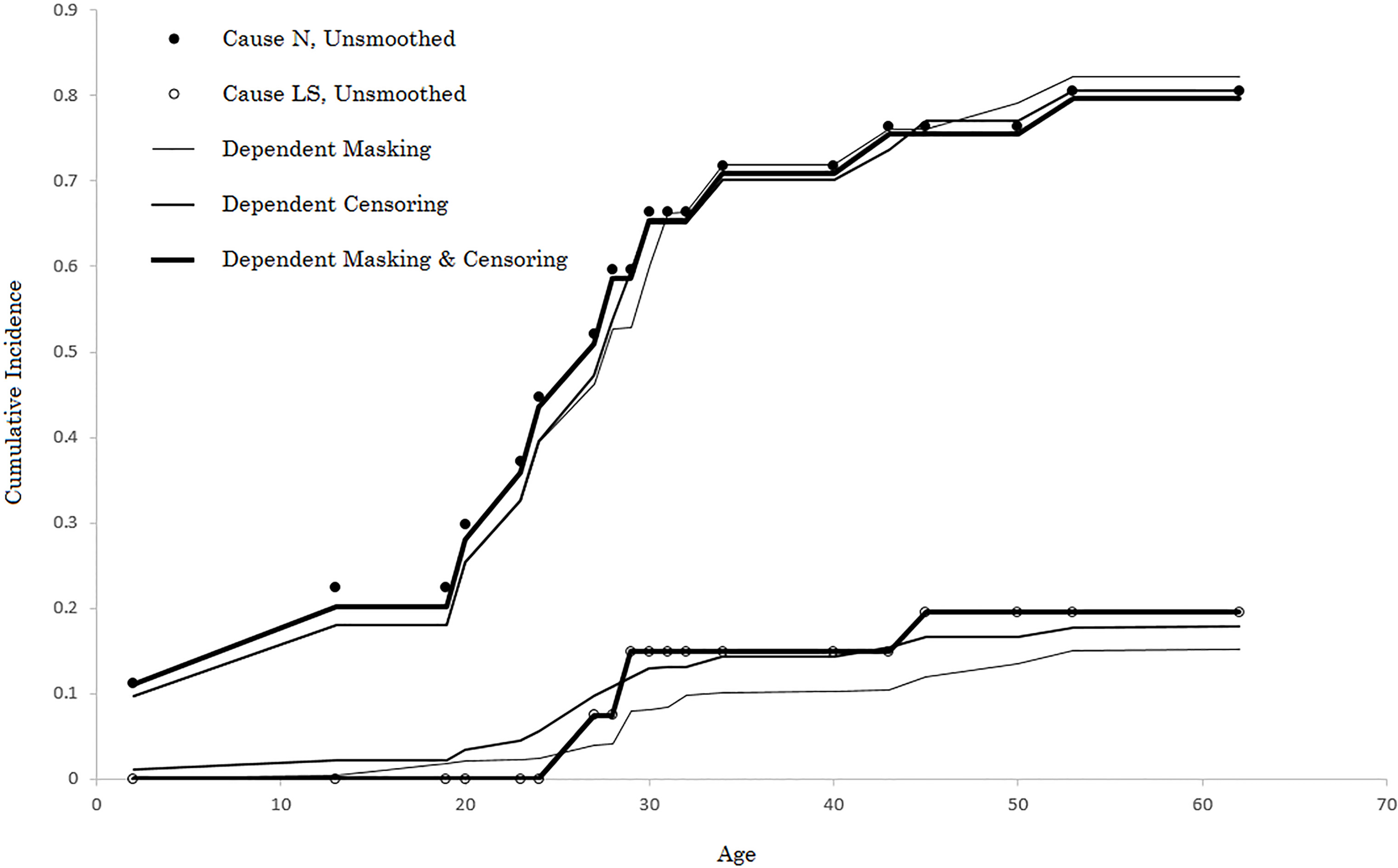
The first set of results are shown under the “Dep Masking” subheading in Table 2, with the result rounded to the nearest one-thousandth. Note that the innermost intervals are no longer present (the few zeros that remain, to the nearest one-thousandth, are due to their numbers being very small; they are not nil). In particular, for cause LS, so many more meaningful failure probabilities are now available, that have the additional benefit of drawing on the dependence between the type of masking and the failure time. Indeed, the lymphatic-sanguine (LS) risk was more associated with higher ages of onset of infection than the neurological form, N. Also, note that the magnitudes of the failure probabilities are themselves revealing. For example, consider age 50. Before the kernel modification, it was not known whether failure due to cause N or cause LS was more likely (since they were both zero). Now, we can estimate that infection at age 50 is over twice as likely to be due to form N than form LS.
The next Kernel Regression was fit to only the censoring-type expressed in terms of regressors, the results being summarized under the subheading, “Dep Censoring” in Table 2. Creating the regressors was yet again not difficult, as there were only left-censored and exact observations for this specific data set (that is, indicator variables sufficed). As can be deduced from a cursory inspection of the data, left-censoring was far more common than exact observations at the higher ages, on average. As such, accounting for this by utilizing a dependent smoothing mechanism is advantageous, leading to more accurate estimates of the failure probabilities than by simply using an independent kernel approach. Interestingly, the results for cause N under dependent censoring exhibited almost the same results as under dependent masking, especially at the lower ages.
Table 3
MMR dependence model results
| Age | Unsmoothed | Dep masking | Dep censoring | Dep mask/cens | ||||
|---|---|---|---|---|---|---|---|---|
|
|
|
|
|
|
|
|
|
|
| 2 | 0.112 | 0.000 | 0.096 | 0.005 | 0.092 | 0.007 | 0.095 | 0.005 |
| 13 | 0.112 | 0.000 | 0.081 | 0.001 | 0.079 | 0.010 | 0.085 | 0.004 |
| 19 | 0.000 | 0.000 | 0.031 | 0.030 | 0.029 | 0.000 | 0.007 | 0.010 |
| 20 | 0.075 | 0.000 | 0.073 | 0.000 | 0.070 | 0.012 | 0.078 | 0.004 |
| 23 | 0.075 | 0.000 | 0.069 | 0.000 | 0.067 | 0.012 | 0.075 | 0.004 |
| 24 | 0.075 | 0.000 | 0.067 | 0.000 | 0.065 | 0.013 | 0.074 | 0.003 |
| 27 | 0.075 | 0.075 | 0.046 | 0.030 | 0.098 | 0.041 | 0.081 | 0.058 |
| 28 | 0.075 | 0.000 | 0.062 | 0.000 | 0.061 | 0.014 | 0.071 | 0.003 |
| 29 | 0.000 | 0.075 | 0.000 | 0.059 | 0.053 | 0.018 | 0.006 | 0.065 |
| 30 | 0.068 | 0.000 | 0.085 | 0.000 | 0.052 | 0.018 | 0.076 | 0.000 |
| 31 | 0.000 | 0.000 | 0.058 | 0.000 | 0.015 | 0.000 | 0.030 | 0.000 |
| 32 | 0.000 | 0.000 | 0.014 | 0.025 | 0.013 | 0.000 | 0.000 | 0.009 |
| 34 | 0.054 | 0.000 | 0.066 | 0.008 | 0.040 | 0.023 | 0.063 | 0.006 |
| 40 | 0.000 | 0.000 | 0.008 | 0.000 | 0.004 | 0.000 | 0.006 | 0.000 |
| 43 | 0.046 | 0.000 | 0.043 | 0.000 | 0.042 | 0.018 | 0.056 | 0.002 |
| 45 | 0.000 | 0.046 | 0.000 | 0.021 | 0.040 | 0.018 | 0.019 | 0.039 |
| 50 | 0.000 | 0.000 | 0.016 | 0.023 | 0.000 | 0.001 | 0.000 | 0.000 |
| 53 | 0.042 | 0.000 | 0.012 | 0.022 | 0.024 | 0.024 | 0.019 | 0.027 |
| 62 | 0.000 | 0.000 | 0.000 | 0.000 | 0.000 | 0.000 | 0.000 | 0.000 |
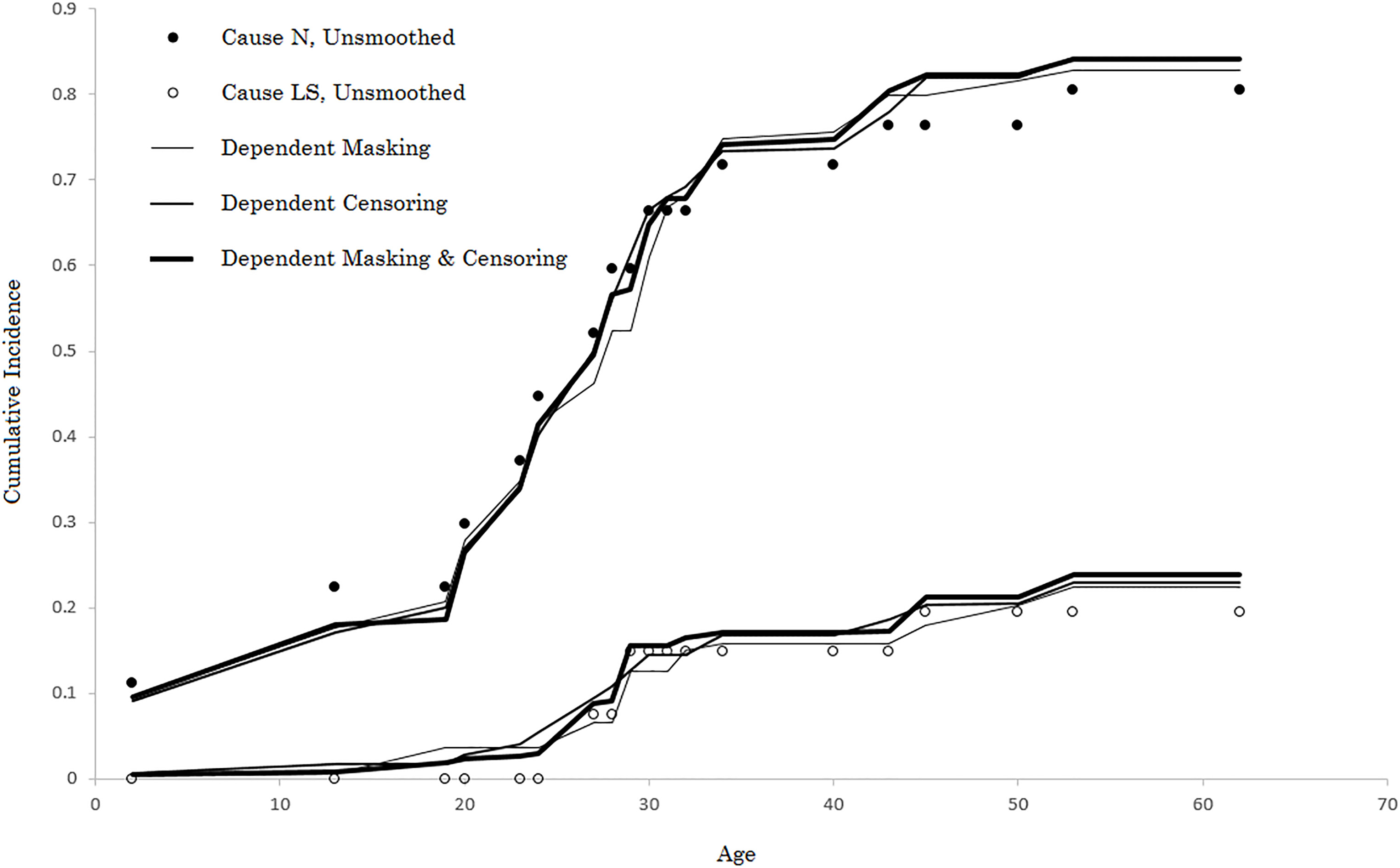
Figure 2.
Converged CIF’s for the MMR dependence models.
The final Kernel Regression was fit to all of the created regressors, whether masking-based or censored-based. The final two columns of Table 2 furnish the results. The probability distribution seems very consistent with the results from the previous two model fits for cause N. However, for cause LS, there was virtually no smoothing that ensued. One possible explanation for this might be over-parameterization of the model in this case (i.e. too many regressors for a relatively small number of data points); but this theory is inconclusive. Figure 1 depicts all of the final CIF curves for all three Kernel Regression fits.
The entire process can be performed again, this time using MMR instead of Kernel Regression. Table 3 illustrates the results. The results from the MMR fits were similar in many ways to the kernel approach, but different in other respects. In terms of similarities, the results for cause N mimic quite closely the pattern exhibited from the kernel approach: the probability distributions were roughly equivalent and the dependent masking and censoring fit again produced similar results to when just masking or just censoring information is utilized. However, the results were very different for cause LS: less smoothing transpired for the MMR models fits when only censoring or only masking information were used, whereas more smoothing emerges for the MMR fits when both masking and censoring were employed in aggregate. Figure 2 plots all of the resulting MMR fits.
The main advantages of the MMR approach over a kernel-based method are (a) ease of understanding; (b) ease in adopting further enhancements such as adding, say, interaction terms between the created masking and censoring covariates, if desired; and (c) computational efficiency. Indeed, this was corroborated by experience, as the algorithms converged much more quickly using the MMR approach. The main advantage of the Kernel Regression over the MMR approach is that it is entirely nonparametric, with the user not required to make any distributional/parametric assumptions whatsoever.
6.Conclusion
The purpose of this paper was to relax the restrictive independence assumption commonly invoked between failure times and the censoring and masking variables found in nonparametric competing risks modeling. This was achieved by incorporating dependent smoothing of the cause-specific failure time density into the SC-CR paradigm, while maintaining the statistical attribute of self-consistency. Dependence was incorporated between the failure times and both the censoring times and the masked causes by employing both Kernel Regression and Multivariate Multiple Regression at each iteration of the SC-CR Algorithm. Our approach to modeling the CIF’s in a multiple decrement setting is intended to be the most automated and data-driven approach possible, and in this respect is unrivaled in the literature to date.
7.Future work
In terms of future work, we note first that the dependent smoothing enhancements can also be incorporated into the interval-censored version of the SC-CR Algorithm of Adamic et al. (2010). This would represent a valuable contribution to the literature, as interval-censoring is extremely commonplace in practice. A second avenue to explore would be whether or not a multivariate copula approach could be used to account for the dependence between failure times with censoring and/or masking, as opposed to the regression approaches we have adopted in the present work. We have already made reference in the introduction to active research in copula-based competing risks scholarship, and a thorough investigation as to whether these methods can be used in the SC-CR framework is certainly warranted. Specifically, the use of a fully nonparametric copula would be in keeping with our goals to provide models that require the least number of assumptions for the analyst. Some research in this regard in the survival analysis sphere has already begun to take shape; a good example is Gribkova and Lopez (2015), who espouse a nonparametric copula approach under bivariate censoring.
Acknowledgments
This work was supported by the Government of Canada, Natural Sciences and Engineering Research Council of Canada under a 2017 Discovery Grant, RGPIN-2017-05595: Actuarial Modeling of Competing Risks Under Various Dependence Structures.
References
[1] | Aalen, O., ((1976) ). Nonparametric inference in connection with multiple decrement models. Scandinavian Journal of Statistics, 3: , 15-27. |
[2] | Adamic, P., ((2010) ). Modeling Multiple Risks in the Presence of Double Censoring. Scandinavian Actuarial Journal, 2010: (1), 68-81. |
[3] | Adamic, P., Dixon, S., & Gillis, D., ((2010) ). Multiple Decrement Modelling in the Presence of Interval Censoring and Masking. Scandinavian Actuarial Journal, 2010: (4), 313-327. |
[4] | Adamic, P., & Guse, J., ((2016) ). LOESS smoothed density estimates for multivariate survival data subject to censoring and masking. Annals of Actuarial Science, 10: (2), 285-302. |
[5] | Braun, J., Duchesne, T., & Stafford, J.E., ((2005) ). Local likelihood density estimation for interval censored data. The Canadian Journal of Statistics, 33: (1), 39-60. |
[6] | Dempster, A.P., Laird, N.M., & Rubin, D.B., ((1977) ). Maximum likelihood from incomplete data via the EM algorithm. Journal of the Royal Statistical Society, Series B, 39: , 1-38. |
[7] | Dinse, G.E., ((1982) ). Nonparametric estimation for partially-complete time and type of failure data. Biometrics, 38: (2), 417-431. |
[8] | Duchesne, T., & Stafford, J.E., ((2001) ). A kernel density estimate for interval censored data. Technical Report No. 0106, University of Toronto. |
[9] | Goutis, C., ((1997) ). Nonparametric estimation of a miixing density via the kernel method. Journal of the American Statistical Association, 92: , 1445-1450. |
[10] | Gribkova, S., & Lopez, O., ((2015) ). Non-parametric copula estimation under bivariate censoring. Scandinavian Journal of Statistics, 42: , 925-946. |
[11] | Groeneboom, P., Maathuis, M.H., & Wellner, J.A., ((2008) ). Current Status Data with Competing Risks, Consistency and Rates of Convergence of the MLE. The Annals of Statistics, 36: , 1031-1063. |
[12] | Hudgens, M.G., Satten, G.A., & Longini, I.M., Jr. ((2001) ). Nonparametric maximum likelihood estimation for competing risks survival data subject to interval censoring and truncation. Biometrics, 57: , 74-80. |
[13] | Jewell, N.P., Van Der Laan, M., & Henneman, T., ((2003) ). Nonparametric estimation from current status data with competing risks. Biometrika, 90: , 183-197. |
[14] | Kalbfleisch, J.D., & Prentice, R.L., ((1980) ). The Statistical Analysis of Failure Time Data. Wiley, New York. |
[15] | Klein, J.P., & Moeschberger, M.L., ((1997) ). Survival Analysis, Techniques for Censored and Truncated Data. Springer, New York. |
[16] | Legros, F., Ancelle, T., & Le réseau A., ((2006) ). Trypanosomiase humaine africaine, recensement des cas d’importation observés en France, 1980–2004. Bulletin épidémiologique Hebdomadaire, 7: , 57-59. |
[17] | Li, L., Watkins, T., & Yu, Q., ((1997) ). An EM algorithm for smoothing the self-consistent estimator of survival functions with interval-censored data. Scandinavian Journal of Statistics, 24: , 531-542. |
[18] | Li, J., & Yu, Q., ((2016) ). A consistent NPMLE of the joint distribution function with competing risks data under the dependent masking and right-censoring model. Lifetime Data Analysis, 22: (1), 63-99. |
[19] | Li, Q., & Racine, J.S., ((2003) ). Nonparametric estimation of distributions with categorical and continuous data. Journal of Multivariate Analysis, 86: , 266-292. |
[20] | Li, Q., & Racine, J.S., ((2004) ). Cross-validated local linear nonparametric regression. Statistica Sinica, 14: , 485-512. |
[21] | Pan, W., ((2000) ). Smooth estimation of the survival function for interval censored data. Statistics in Medicine, 24: , 531-542. |
[22] | Racine, J.S., & Li, Q., ((2004) ). Nonparametric estimation of regression functions with both cate-gorical and continuous data. Journal of Econometrics, 119: , 99-130. |
[23] | Stafford, J., ((2005) ). Exact’ Local Likelihood Estimators. http,//www.gla.ac.uk/external/RSS/RSScomp/Stafford.pdf [accessed Jan 25 2018]. |
[24] | Turnbull, B.W., ((1974) ). Nonparametric estimation of a survivorship function with doubly censored data. Journal of the American Statistical Association, 69: , 169-173. |
[25] | Turnbull, B.W., ((1976) ). The empirical distribution function with arbitrarily grouped, censored and truncated data. Journal of the Royal Statistical Society, 38: , 290-295. |
Appendices
Appendix
Proof that E[E[X
Proof that E[E[X
Let
Thus, it follows that


