
IntelliScan: Improving the quality of x-ray computed tomography surface data through intelligent selection of projection angles
Abstract
X-ray computed tomography (XCT) enables the dimensional measurement and inspection of highly geometrically complex engineering components that are unmeasurable using optical and tactile instruments. Conventional XCT scans use a circular scan trajectory where X-ray projections are acquired with a uniform angular spacing; this approach treats all projections as being of equal importance, in practice, some projections contain more object information than others. In this work we capitalize on this concept by intelligently selecting projections with a view to improve the quality of surface models extracted from an XCT data-set. Our approach relies on using a priori object information to select X-ray projections in which the surfaces of the object are aligned with a ray-path, thus ensuring the surface of the object is fully sampled. Results are presented showing that the proposed method is able to reduce CAD comparison errors by 16%, reduce surface form error by 3%, and improve edge contrast by 14% for a machined aluminium component.
1Introduction
X-ray computed tomography (XCT) is increasingly used as a measurement tool for verifying that engineering components have been made correctly. XCT is particularly well-suited for the measurement and inspection of metal additively manufactured components, as it enables the measurement of inaccessible internal features that are unmeasurable using tactile and optical methods.
Since its invention, XCT systems have mostly utilized a circular scan trajectory, whereby either the object to be scanned is rotated between a stationary X-ray source and detector, as per industrial XCT scanners, or the X-ray source and detector rotate around a stationary object, as per medical XCT scanners. The popularity of the circular scan trajectory is perhaps due to its simplicity, combined with the mathematics underpinning Fourier-based reconstruction algorithms. Most practitioners will agree that for the vast majority of cases, a circular scan trajectory leads to an acceptable quality of XCT data. However, as engineering components become more geometrically complex due to advances in manufacturing technology, perhaps more exotic XCT scan trajectories may offer some advantages [1–4].
Computer aided design (CAD) data is almost always available for modern engineering components; it seems illogical to ignore the information provided by a CAD model when planning an XCT scan. Additional information such as the material of the component should also be readily available.
The concept of using a priori object information to improve the quality of XCT reconstructions is not new. A review of the literature shows that a number of methods for optimizing the XCT scan strategy based on a priori object information have been proposed [5–13]. These approaches generally aim to select an optimal object scan orientation, or source-detector scan trajectory; this is achieved by simulating projections for all possible object orientations, and then selecting the object orientation or source-detector trajectory that maximizes some quality metric. This general approach is clearly computationally expensive, and not all end users have access to XCT simulation tools which will stifle adoption.
Heinzl et al. [5] selected an optimal scan orientation of an object by evaluating material penetration lengths and the completeness of Radon sampling from simulations of the object in all possible orientations. Fischer et al. [6] developed an algorithm to select the optimal projection angle for a given object feature; the optimality of a projection is quantified by evaluating the modulation transfer function and the noise power spectrum of the system matrix of an iterative reconstruction algorithm. Ito et al. [7] selected an optimal object scan orientation by simulating projections of all possible object orientations and evaluating metrics indicative of metal artifacts, beam hardening artifacts and cone-beam artifacts, the object orientation that simultaneously minimised the metrics was selected as optimal; aspects of this approach were further developed in [8] to include the fusion of multiple XCT data sets in order to minimise metal artifacts. Herl et al. [9] developed a method to select projection angles to reconstruct a region of interest of an object using a dual robot XCT system; the completeness of Radon sampling and material penetration lengths were used to select projections from a set of candidate projections. Herl et al. further developed their method in [10] by investigating the use of an alternative quality metric based on the modulation transfer function and noise power spectrum of the reconstruction, which has also been utilised in recent work by Bauer et al. [12].
The main limitation of many of the studies referenced above is that exhaustive simulations of an object in all possible scan orientations or scan trajectories must be conducted. We propose to overcome this by simply inspecting the features of an object and then calculating the projection angles required to reconstruct them; no exhaustive XCT simulation is required, nor an optimisation algorithm. The aim of our method is to improve the quality of object surfaces, such that a surface model of an object can be extracted from a CT data set for subsequent analysis [14, 15]. Our approach is inspired by that of Zheng et al. [11] and Qunito et al. [13] who noted that the surface of an object can only be reliably reconstructed if a ray-path is tangent to the surface; this was also recently exploited by Butzhammer et al. [16]. Therefore, we propose to focus on selecting projections that contain X-rays that are tangent to the object’s surfaces; we hereafter refer to this approach as IntelliScan.
It is worth noting that a body of work exists on seeking to optimize XCT and MRI scans on-the-fly, i.e. the next image to be acquired in a scan is estimated based on the projection set and partial reconstruction currently available [17–21]; this is not the focus of the present work. It is assumed throughout this work that the object to be scanned is known by means of an engineering drawing or CAD model, thus the projection selection can be undertaken offline, before scanning takes place.
2Methodology
The methodology adopted is as follows: the general approach for intelligently selecting projection angles is first described (Section 2.1); a suitable test sample is selected to demonstrate the proposed method (Section 2.2); the application of the general approach to the test sample is described (Section 2.3), XCT scan conditions and data processing methods are described (Section 2.4); and results presented (Section 3).
2.1Projection selection approach
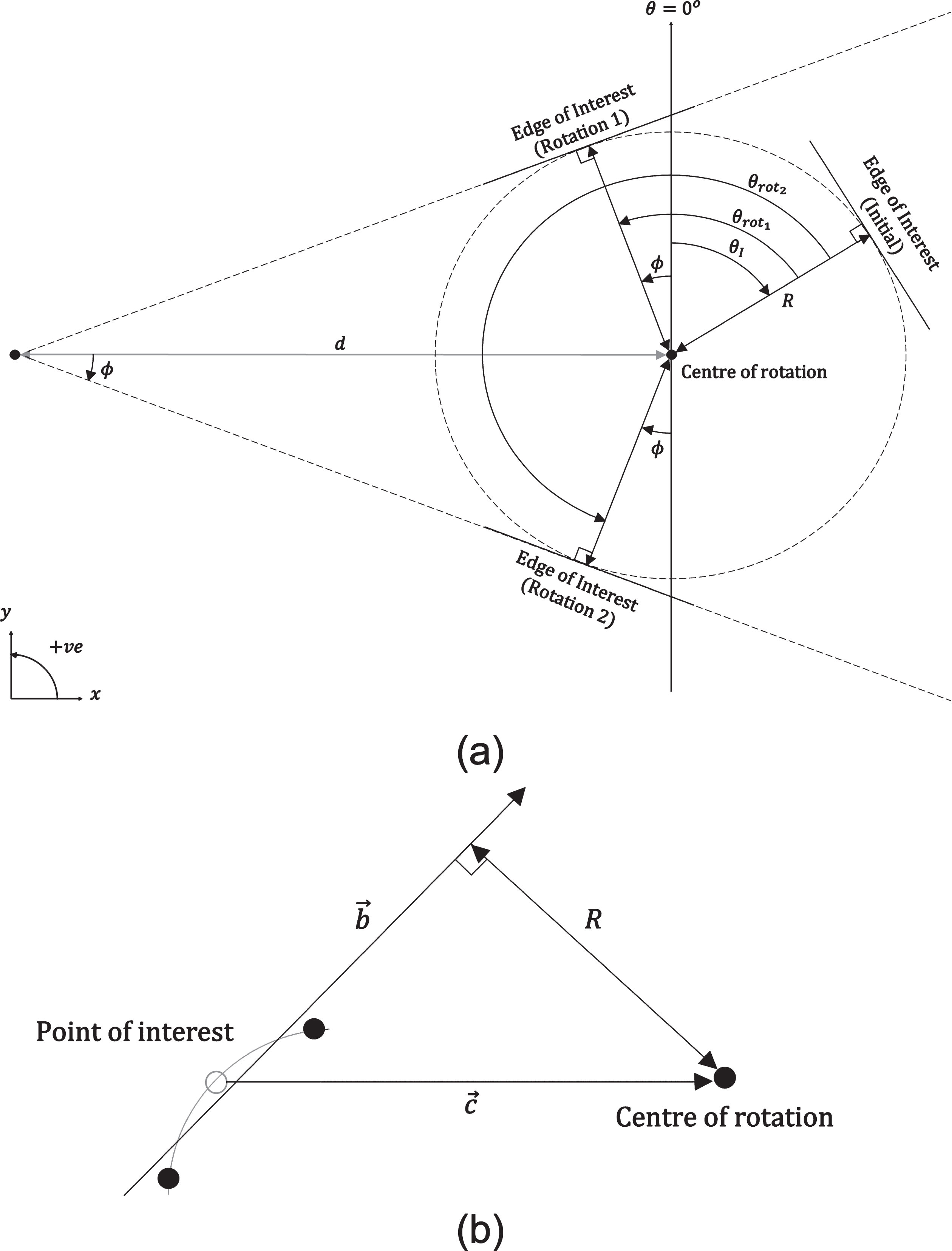
Assuming a flat detector, and a ray-path from the source to each detector pixel, there are two projection angles where ray-paths are tangent to a given edge in the XY plane, θrot1 and θrot2, see Fig. 1a. The projection angles θrot1 and θrot2 can be calculated by determining the initial rotation of an edge, θI, and the angle at which the considered edge is aligned with a ray-path, φ and 180o - φ respectively:
(1)
(2)
Assuming the sample is rotated about its geometric center, let R be the perpendicular distance from the sample’s center of rotation to the considered edge. Furthermore, let the distance from the X-ray focal spot to the sample’s center of rotation be d. The angle at which the edge of interest is aligned with a ray-path, φ, is calculated as:
(3)
The above approach only considers edges; let us now consider an arbitrary point that lies on a curve. The projection angle required for a given point is calculated in the same way as for an edge, although R is calculated as the cross product of the point’s local direction,
(4)
Fig. 1
(a) Illustration of the projection selection method with the edge of interest highlighted. (b) Illustration of projection selection method for a point on a curve; the point direction is perpendicular to the surface normal.
2.2Test sample
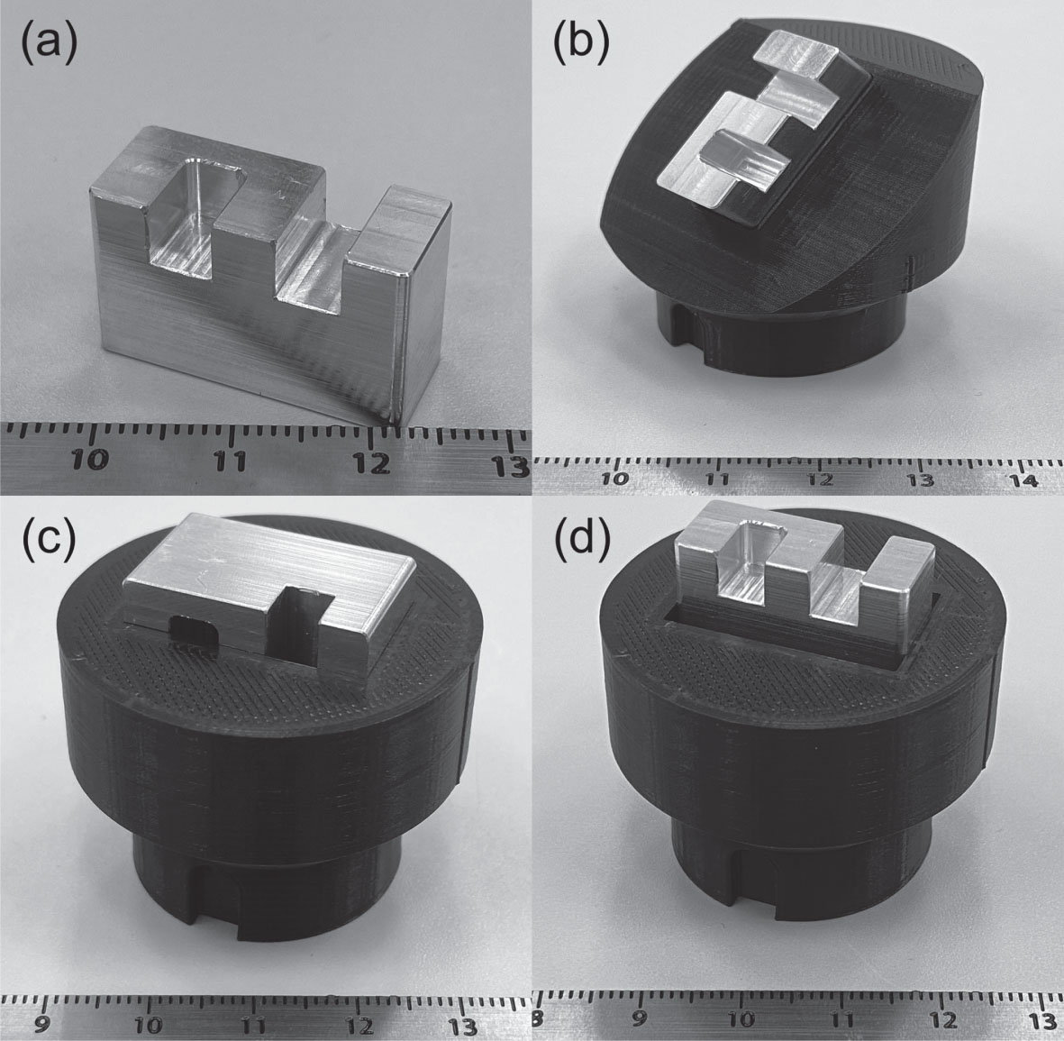
To demonstrate the proposed method a test sample is selected, see Fig. 2a. The test sample is nominally 25 mm x 15 mm x 10 mm (L x H x D) in size and is fabricated from aluminium. The test sample has 14 faces, 25 edges, and 14 corners; CAD data and a technical drawing of the test sample are available and are used to assist in calculating the IntelliScan projection angles.
Fig. 2
(a) Photo of the test sample. (b) Test sample in the conventional scan orientation. (c) Test sample in the horizontal orientation. (d) Test sample in the vertical orientation.
2.3Application of the projection selection approach to the test sample
In order to analyze the performance of our proposed approach, a benchmark scan of the test sample is conducted using a conventional scanning approach. For the conventional scan, the test sample is orientated with a 45-degree inclination as shown in Fig. 2b and 360 evenly spaced projections are acquired.
In order to apply our IntelliScan approach to the test sample, two orthogonal scans are required, see Fig. 2c and 2d respectively. Due to the geometric simplicity of the test sample, the IntelliScan angles are evaluated from a simplified technical drawing, see Fig. 3. When the sample is in the vertical orientation there are 9 faces that can be aligned with ray-paths, hence 18 projection angles are calculated. When the sample is in the horizontal orientation, another 9 faces can be aligned with ray-paths, hence another 18 projection angles are calculated.
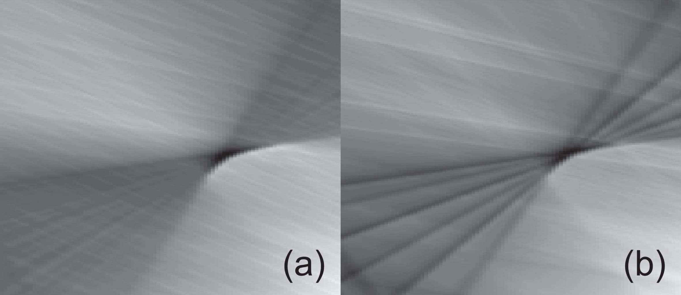
When the sample is in the horizontal orientation, there are 6 corners of radius 1 mm (Fig. 3a). We choose to use 6 projection angles per corner, so 36 projections to capture the corners of the sample in the horizontal orientation. When the sample is in the vertical orientation (Fig. 3b), there are 8 corners of radius 0.5 mm. We choose to use 4 projection angles per corner, so 32 projections to capture the corners of the sample in the vertical orientation. The number of projections per corner is chosen based on a simulation study that showed good quality corner reconstructions are possible with as few as 6 and 4 projections for the horizontal and vertical sample orientations respectively, see Fig. 4a and Fig. 4b respectively.
A total of 54 intelligently selected projection angles are chosen for the horizontal sample orientation, and 50 for the vertical sample orientation. To ensure both the conventional scan and IntelliScan use the same number of projections, a further 126 projections need to be selected in the horizontal orientation and 130 in the vertical orientation. The remaining projection angles are selected as follows: the largest angular gap between two successive projections is found and a projection is added at the angular midpoint, this is repeated until all the 180 projections are allocated. These additional projections are used here to ensure a fair comparison between the conventional scan and IntelliScan; it would be an unfair comparison if the total number of projects acquired in each scan was not the same. The additional projections are not expected to contribute additional edge information to the reconstruction. Users are free to omit these projections if they are deemed not necessary, perhaps due to a desire to minimise scan time
The initial orientation of the test sample is set by designing a slot in the sample mount that mates with the grub screw of the XCT system’s rotation stage; the slot is visible in Figs. 2c and 2d. The rudimentary mechanical alignment provided by the slot and grub screw is sufficient to provide the desired initial sample orientation, θI. The angular misalignment of the sample is evaluated from the reconstructed data and found to be approximately 0.26 degrees. In a similar manner, the sample mount was designed such that the sample’s centre of rotation and the XCT system’s rotation axis were aligned.
Fig. 3
Illustration showing (a) 9 faces (V) and 6 corners (VC) of the test sample identified in the vertical orientation, (b) 9 faces (H) and 8 corners (HC) of the test sample identified in the horizontal orientation. The centre of rotation shown into the page.
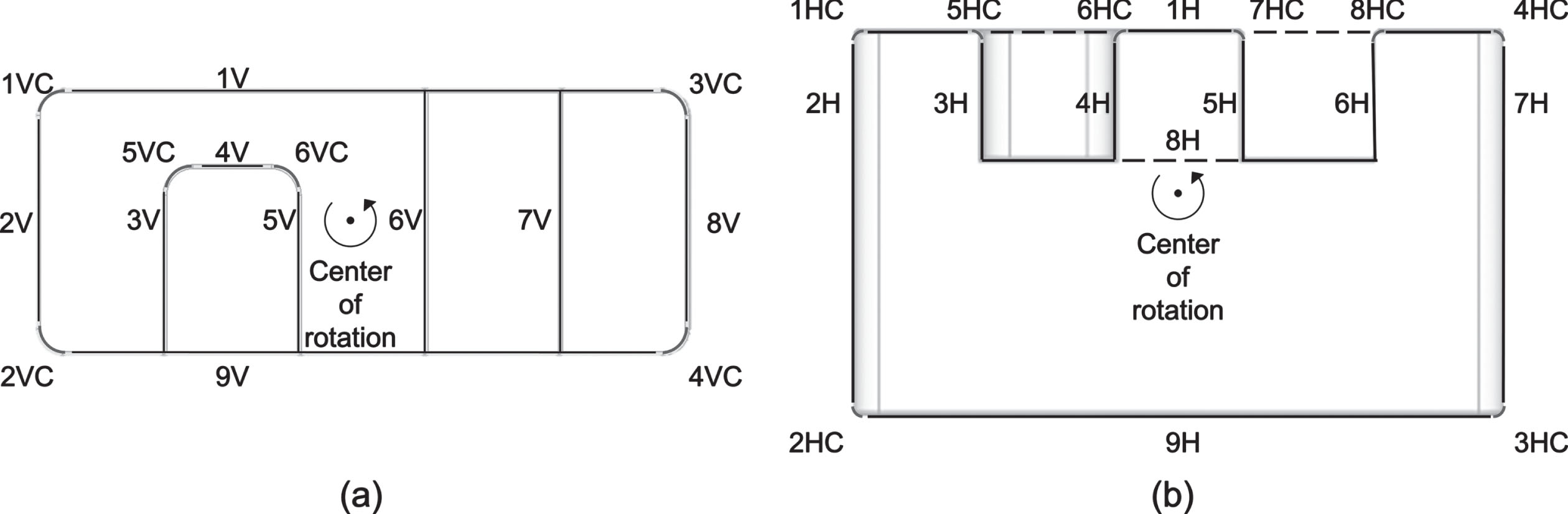
Fig. 4
CT slice showing a corner reconstructed using: a) 22 projections, b) 6 projections. Based on simulated data.
2.4XCT system, reconstruction and data processing
The XCT system used is a Nikon XT H 225 ST. The system uses a microfocus X-ray source with an acceleration voltage of 200 kV, a filament current of 200 μA. The system consists of a flat panel detector with an active area of 400 mm by 400 mm, a pixel matrix of 2000 by 2000 pixels and a pixel size of 0.2 mm. The test sample is scanned with a voxel size of 0.04 mm, with d = 223.2 mm. The X-ray spectrum is pre-filtered with 0.5 mm of copper. The detector exposure time is set to 2 seconds, with a gain of 18 dB. Each projection is acquired fourfold and averaged to reduce measurement noise.
All reconstructions are performed using an in-house implementation of the filtered backprojection algorithm [22]. The conventional filtered backprojection algorithm assumes that the object undergoes uniform angular sampling; a modified filtered backprojection algorithm for non-uniformly sampled data was developed by Zeng et al. [23]. However, based on our experiments, we find that the conventional filtered backprojection algrorithm works well without modification. The orthogonal scans for the IntelliScan method are reconstructed separately. The IntelliScan reconstructions are merged by first determining the test sample’s surfaces, then aligning the data to a CAD model, the two aligned CT volumes are then averaged and the surface of the merged data is re-evaluated. If there are artifacts in the XCT data that propagate through to the determined surface, then registering the surfaces to the CAD model may be problematic [24], however, this was not observed in this work. All the data processing is performed in Volume Graphics VGSTUDIO MAX 3.5 (Volume Graphics GmbH, Heidelberg, Germany) and GOM Inspect (Carl Zeiss GOM Metrology GmbH, Braunschweig, Germany).
3Results
The surface of each reconstruction is determined and aligned with the CAD model of the test sample. The deviation of the reconstructed data from the CAD model is visualized for the conventional scan and IntelliScan, see Fig. 5a and 5b respectively; the colourmap is a visualisation of the the surface deviation between the CAD surface and XCT surface. IntelliScan has a total surface deviation of 14.6 mm3, whilst the conventional scan has a total surface deviation of 17.4 mm3; this is a 16% decrease in total surface deviation. This result is largely due to the conventional scan having blurred corners compared to IntelliScan, as shown in Fig. 5a. It should be noted that this analysis is based on the assumption that the test sample is free of manufacturing defects, hence the CAD model is representative of the test sample.
Fig. 5
(a) Visualisation of surface deviation from CAD model for a conventional scan. (b) Visualisation of surface deviation from CAD model for an IntelliScan. Large deviations are seen for the corners of the conventional scan compared to IntelliScan. It is assumed that the test sample is free of manufacturing defects and the CAD model is representative of the test sample.
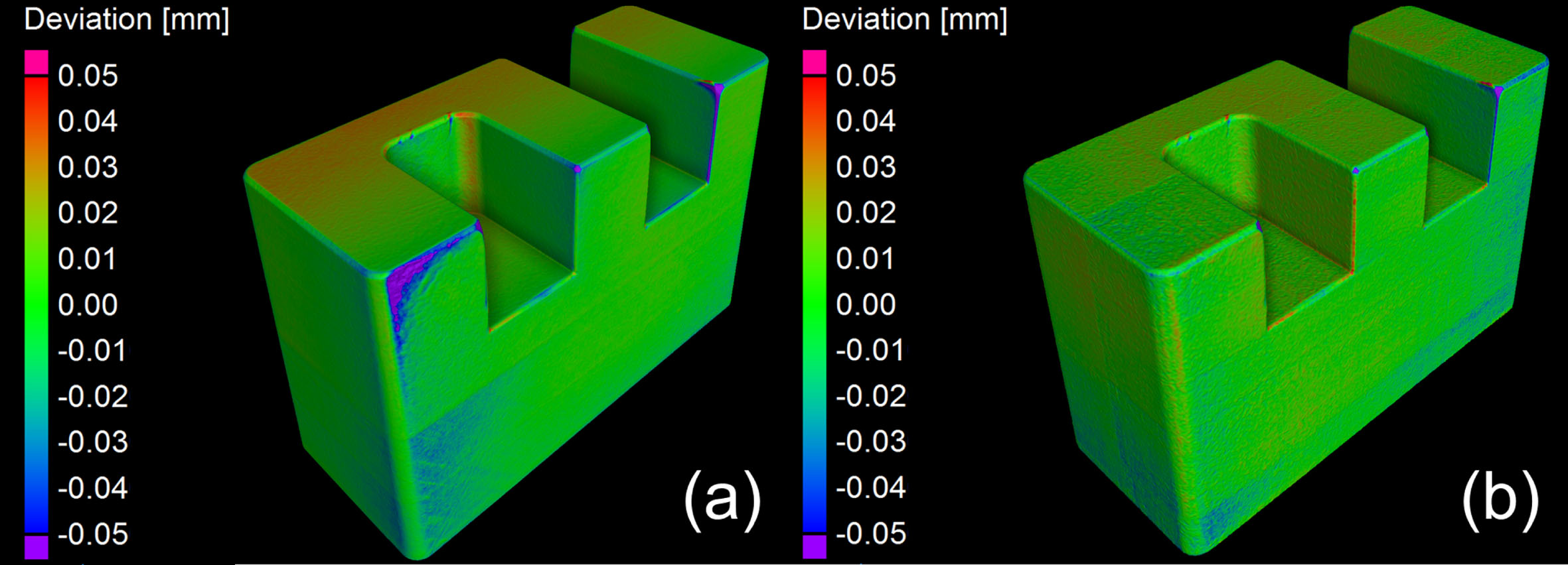
Fig. 6
Slice along XY plane for (a) conventional scan, (b) IntelliScan. Slice along XZ plane for (c) conventional scan, (d) IntelliScan.
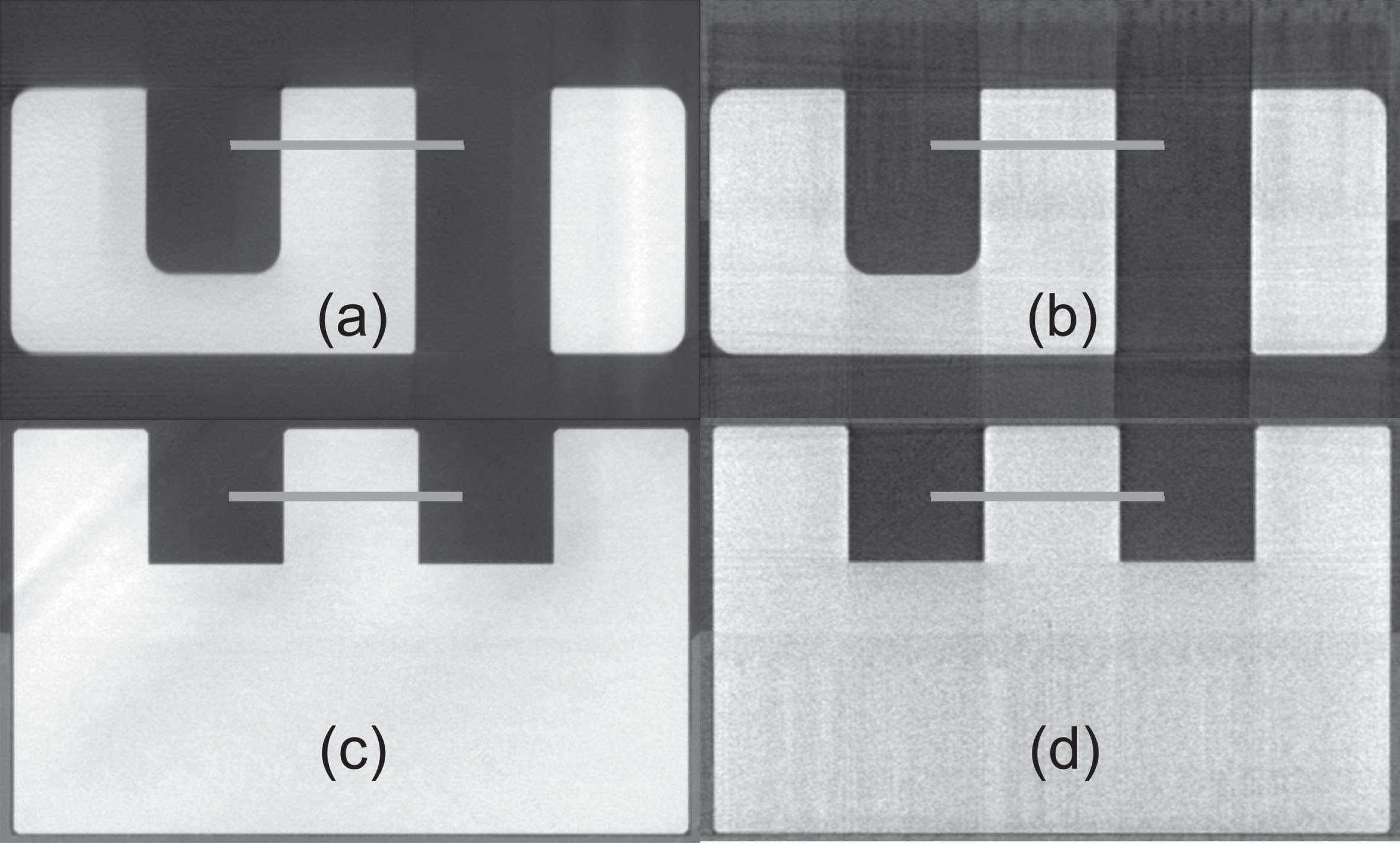
CT slices for each reconstruction are shown in Fig. 6. Line profiles evaluated from the slices are shown in Fig. 7. The line profiles show that the edge contrast is greater for IntelliScan when compared to the conventional scan. The edge contrast is calculated as the maximum grey value gradient across each edge; the absolute grey value gradient for the line profiles are shown in Fig. 7c and 7d. The mean edge contrast from the line profiles is 1.27 for IntelliScan and 1.11 for the conventional scan; this is an increase of edge contrast of 14%.
Fig. 7
Grey value line profiles and grey value gradient evaluated from Fig. 6 (a) and (c) XY slice, (b) and (d) XZ slice. Note that the grey value gradient for IntelliScan in plots (c) and (d) has been shifted by 3 pixels in order to clearly show the change in gradient magnitude.
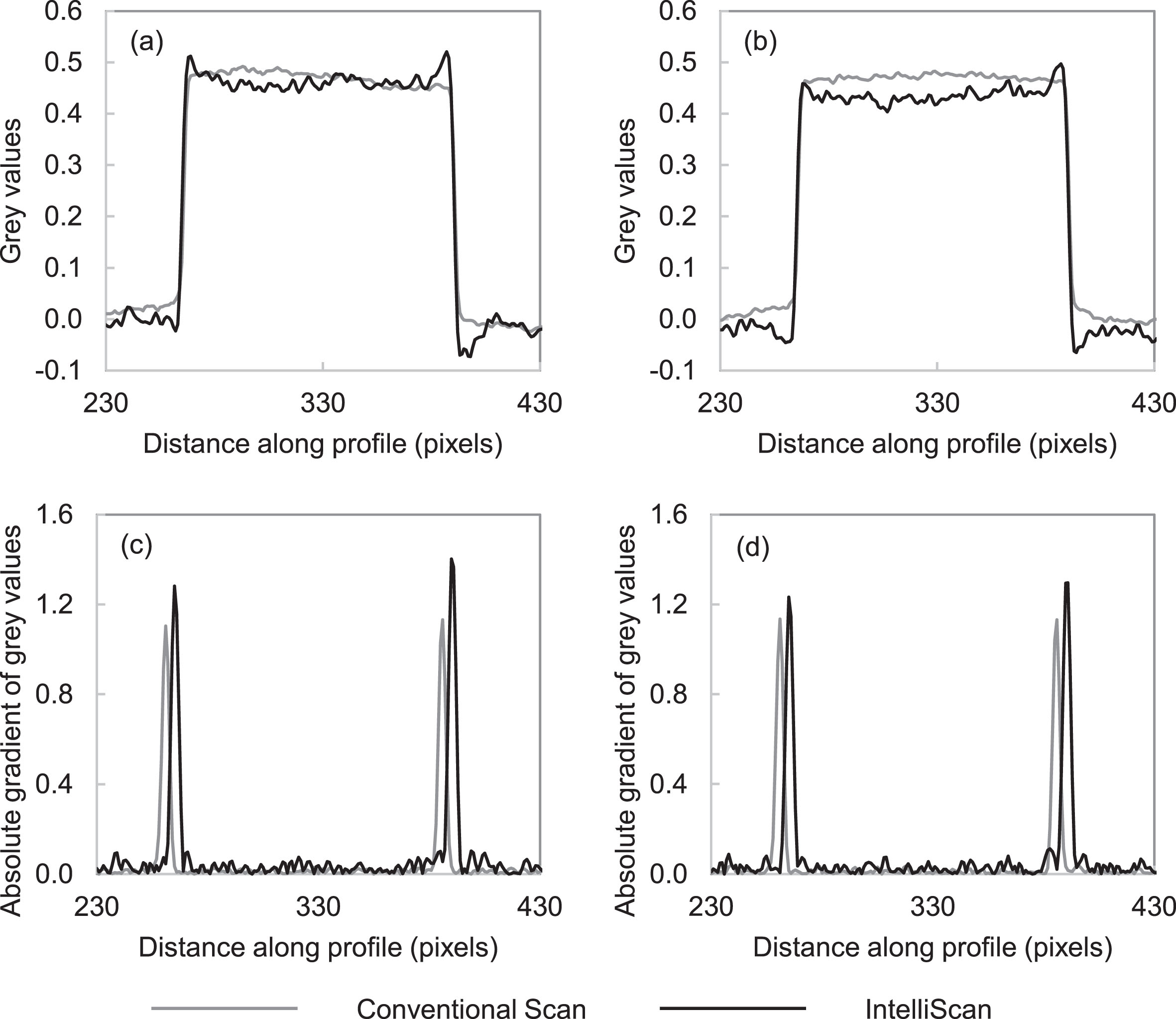
Fig. 8
(a) Visualisation of planar deviation for a face of the conventional scan result. (b) Visualisation of planar deviation for a face of the IntelliScan result.
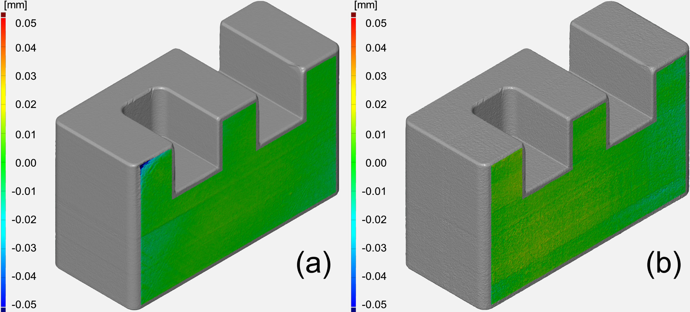
Planes are fitted to the 14 faces of the test sample. For each reconstruction, the form deviation of each plane is evaluated. An example is shown in Fig. 8 for a single plane. The sum of the form error for all 14 planes is 1.09 mm for IntelliScan and 1.12 mm for the conventional scan; a reduction of form error by 3%.
4Discussion and conclusions
For the considered test sample, the proposed approach for intelligently selecting projection angles reduced the reconstructed surface deviation from the CAD model by 16%, improved the edge contrast by 14%, and reduced surface form error by 3%. These results are limited to the case considered, but illustrate the gains that can be achieved with slight modifications to the scan strategy. It is important to highlight that no excessive XCT simulations or complex optimization algorithms are required in the proposed approach; we simply select particular projection angles based on a priori knowledge of the object to be scanned.
The obvious disadvantage of the method, for the test sample considered, is the need to scan the sample in two orientations to capture all the surfaces; this will lead to a slight increase in scan time as the operator will need to remove the sample and change its orientation. This is a consequence of our method considering only the alignment of an object’s surfaces with X-rays presented by the central fan-beam of a cone-beam system; we have not considered the possibility of aligning an object’s surfaces with X-rays above or below the central fan-beam. For the test sample considered, the faces of the sample can be aligned with the cone-beam if the sample is inclined in such a way that the plane formed by each face intersects the X-ray source. In future work we will consider how to exploit this property in order to overcome the need to reorient the sample.
The developed method has an important underlying assumption: that the scanned sample and the design data are in close agreement. If the sample to be scanned does not closely match the design data then the projection angles calculated using our method will be incorrect. To overcome this, a modified approach could be used whereby instead of acquiring just the nominal projection angles for each surface, a range of angles are acquired centred around the nominal angle. This approach would catch any surfaces that significantly deviate from the design data, but at a cost of using valuable projection angles. This approach could also address any error in the initial alignment of the sample, i.e. if there is an error in θI or if the sample’s centre of rotation is not aligned with that of the XCT system’s rotation stage.
It could be argued that the conventional scan led to inferior results because too few projections were acquired to reconstruct the sample’s surface correctly. This is true, and the use of a low number of projections was deliberate as it highlights that sharp edges can be reconstructed if the projection angles are intelligently chosen. This has implications for those interested in minimizing scan time; is it necessary to acquire thousands of projections just to reconstruct sharp edges? Is it not more sensible to reduce scan time using well-chosen projections? Reducing the scan time also reduces focal spot drift, which in turn will reduce the blurring of sharp edges in high-resolution scans; this is still advisable even if a focal spot drift correction method is used [25].
This work made use of a Fourier-based reconstruction algorithm. There may be further image quality improvements to be realized through the use of an iterative reconstruction algorithm [26]. The use of such algorithms will be considered in future work, alongside the development of a fully automated implementation of our method, whereby the user inputs a CAD model of the object to be scanned, and all the IntelliScan angles are output, ready for deployment via a robotic object manipulator.
Acknowledgements
This research is supported by A*STAR under its Industry Alignment Fund-Pre Positioning (IAF-PP), Grant number A20F9a0045. Any opinions, findings and conclusions or recommendations expressed in this material are those of the authors and do not reflect the views of A*STAR.
REFERENCES
[1] | Butzhammer L. , Hausotte T. Complex 3d scan trajectories for industrial conebeam computed tomography using a hexapod, Measurement Science and Technology 32: (10) ((2021) ), 105402. 10.1088/1361-6501/ac08c4. URL https://doi.org/10.1088/1361-6501/ac08c4 |
[2] | Fenglin L. , Chao Q. , Weiwen W. , Peng F. , Yufang C. Synchronous scanning mode of industrial computed tomography for multiple objects test, Journal of X-ray Science and Technology 25: (5) ((2017) ), 765–775. 10.3233/XST-16229. URL https://doi.org/10.3233/xst-16229 |
[3] | O’Brien N.S. , Boardman R.P. , Sinclair I. , Blumensath T. Recent advances in xray cone-beam computed laminography, Journal of X-ray Science and Technology 24: (5) ((2016) ), 691707. 10.3233/XST-160581. URL https://doi.org/10.1016/j.jsurg.2016.07.008 |
[4] | Samber B.D. , Renders J. , Elberfeld T. , Maris Y. , Sanctorum J. , Six N. , Liang Z. , Beenhouwer J.D. , Sijbers J. Flexct: a flexible x-ray ct scanner with 10 degrees of freedom, Opt Express 29: (3) ((2021) ), 3438–3457. 10.1364/OE.409982. URL http://opg.optica.org/oe/abstract.cfm?URI=oe-29-3-3438 |
[5] | Heinzl C. , Kastner J. , Amirkhamov A. , Gröller E. , Gusenbauer C. Optimal specimen placement in cone beam x-ray computed tomography, E International 50: ((2012) ), 42–49 https://doi.org/10.1016/j.ndteint.2012.05.002. URL https://www.sciencedirect.com/science/article/pii/S096386951200062X |
[6] | Fischer A. , Lasser T. , Schrapp M. , Stephan J. , Nöel P.B. Object specific trajectory optimization for industrial x-ray computed tomography, Scientific Reports 6: ((2016) ). https://doi.org/10.1038/srep19135 |
[7] | Ito T. , Ohtake Y. , Suzuki H. Orientation optimization and jig construction for xray ct scanning, NDT.net10th 220 Conference on Industrial Computed Tomography, Wels, Austria (2020). |
[8] | Tan Y. , Ohtake Y. , Suzuki H. Scan angle selection and volume fusion for reducing metal artifacts by multiple x-ray ct scanning, Precision Engineering 74: ((2022) ), 384–395. https://doi.org/10.1016/j.precisioneng.2021.07.020 |
[9] | Herl G. , Hiller J. , Maier A. Scanning trajectory optimisation using a quantitative tuybased local quality estimation for robot-based x-ray computed tomography, Nondestructive Testing and Evaluation 35: (3) ((2020) ), 287–303. arXiv: https://doi.org/10.1080/10589759.2020.1774579, doi: 10.1080/10589759.2020.1774579. URL https://doi.org/10.1080/10589759.2020.1774579 |
[10] | Herl G. , Hiller J. , Thies M. , Zaech J.-N. , Unberath M. , Maier A. Task-specific trajectory optimisation for twin-robotic x-ray tomography, IEEE Transactions on Computational Imaging 7: ((2021) ), 894–907 doi: 10.1109/TCI.2021.3102824. |
[11] | Zheng Z. , Mueller K. Identifying sets of favourable projections for few-view lowdose cone-beam ct scanning, Stony Brook University11th International Meeting on Fully Three-Dimensional Image Reconstruction in Radiology and Nuclear Medicine, Potsdam, Germany (2011). |
[12] | Bauer F. , Forndran D. , Schromm T. , Grosse C.U. Practical part-specific trajectory optimization for robot-guided inspection via computed tomography, Journal of Nondestructive Evaluation 41: (3) ((2022) ), 894–907. doi: 10.1137/0524069. URL https://doi.org/10.1137/0524069 |
[13] | Quinto E.T. Singularities of the x-ray transform and limited data tomography in r2 and r3, SIAM J Math Anal 24: (5) ((1993) ), 1215–1225. doi: 10.1137/0524069. URL https://doi.org/10.1137/0524069 |
[14] | Carmignato S. , Dewulf W. , Leach R. Industrial X-Ray Computed Tomography, Springer, Switzerland, (2018) . |
[15] | Villarraga-Gómez H. , Amirkhanov A. , Heinzl C. , Smith S.T. Assessing the effect of sample orientation on dimensional x-ray computed tomography through experimental and simulated data, Measurement 178: ((2021) ), 109343. doi: https://doi.org/10.1016/j.measurement.2021.109343. URL https://www.sciencedirect.com/science/article/pii/S0263224121003390 |
[16] | Butzhammer L. , Hausotte T. Effect of iterative sparse-view ct reconstruction with task-specific projection angles on dimensional measurements, 9th Conference on Industrial Computed Tomography, Padova, Italy (2019). |
[17] | Placidi G. , Alecci M. , Sotgiu A. Theory of adaptive acquisition method for image reconstruction from projections and application to epr imaging, Journal of Magnetic Resonance, Series B 108: (1) ((1995) ), 50–57. doi: https://doi.org/10.1006/jmrb.1995.1101. URL https://www.sciencedirect.com/science/article/pii/S1064186685711016 |
[18] | Haque M.A. , Ahmad M.O. , Swamy M.N.S. , Hasan M.K. , Lee S.Y. Adaptive projection selection for computed tomography, IEEE Transactions on Image Processing 22: (12) ((2013) ), 5085–5095. doi: 10.1109/TIP.2013.2280185. |
[19] | Dabravolski A. , Batenburg K.J. , Sijbers J. Dynamic angle selection in x-ray computed tomography, Nuclear Instruments and Methods in Physics Research Section B: Beam Interactions with Materials and Atoms, 324: ((2014) ). 17–24. 1st International Conference on Tomography of Materials and Structures doi: https://doi.org/10.1016/j.nimb.2013.08.077. URL https://www.sciencedirect.com/science/article/pii/S0168583X14000986 |
[20] | Zibetti M.V.W. , Herman G.T. , Regatte R.R. Fast data-driven learning of mri sampling pattern for large scale problems (2020). doi: 10.48550/ARXIV.2011.02322. URL https://arxiv.org/abs/2011.02322 |
[21] | Thies M. , Zäch J.-N. , Gao C. , Taylor R. , Navab N. , Maier A. , Unberath M. A learning-based method for online adjustment of c-arm cone-beam ct source trajectories for artifact avoidance, International Journal of Computer Assisted Radiology and Surgery 15: (11) ((2020) ). 10.1109/TIP.2013.2280185. |
[22] | Feldkamp L.A. , Davis L.C. , Kress J.W. Practical cone-beam algorithm, J Opt Soc Am A 1: (6) ((1984) ), 612–619. doi: 10.1364/JOSAA.1.000612. URL http://opg.optica.org/josaa/abstract.cfm?URI=josaa-1-6-612 |
[23] | Zeng G.L. A filtered backprojection map algorithm with nonuniform sampling and noise modeling, Medical Physics 39: (4) ((2012) ), 2170–2178. doi: 10.1118/1.3697736. |
[24] | Müller A.M. , Hausotte T. Data fusion of surface data sets of x-ray computed tomography measurements using locally determined surface quality values, Journal of Sensors and Sensor Systems 7: (2) ((2018) ), 551–557. doi: 10.5194/jsss-7-551-2018. URL https://jsss.copernicus.org/articles/7/551/2018/ |
[25] | Bircher B.A. , Meli F. , Küng A. , Sofiienko A. Traceable x-ray focal spot reconstruction by circular edge analysis: from sub-microfocus to mesofocus, Measurement Science and Technology 33: (7) ((2022) ), 074005. doi: 10.1088/1361-2706501/ac6225. URL https://doi.org/10.1088/1361-6501/ac6225 |
[26] | Aarle W.V. , Palenstijn W.J. , Cant J. , Janssens E. , Bleichrodt F. , Dabravolski A. , Beenhouwer J.D. , Batenburg K.J. , Sijbers J. Fast and flexible x-ray tomography using the astra toolbox, Opt Express 24: (22) ((2016) ), 25129–25147. doi: 10.1364/OE.24.025129. URL http://opg.optica.org/oe/abstract.cfm?URI=oe-24-22-25129 |


