
An analysis of curling using a three-dimensional Markov model
Abstract
Using data from 1,199 matches containing 10,933 ends in the Canadian Men’s Curling Championships, we developed both a three-dimensional empirical state space model and three-dimensional homogeneous and heterogeneous Markov models to estimate win probabilities throughout a curling match. The Markovian win probabilities were derived from the observed scoring probabilities using recursive logic.
These win probabilities allowed us to answer questions regarding optimal curling strategy. When presented with the choice to score 1 point or blanking an end, we conclude that teams holding the hammer should choose to blank the end in most situations. Looking at empirical results of conceded matches, we conclude that concession behavior is consistent with a psychological win probability threshold of 2.57%. However, we also find that teams frequently concede when their win probability at time of concession is, in fact, much higher than this threshold. This is true particularly after the 9th end, suggesting that teams are conceding matches when they have up to a 15% chance of winning.
1Introduction
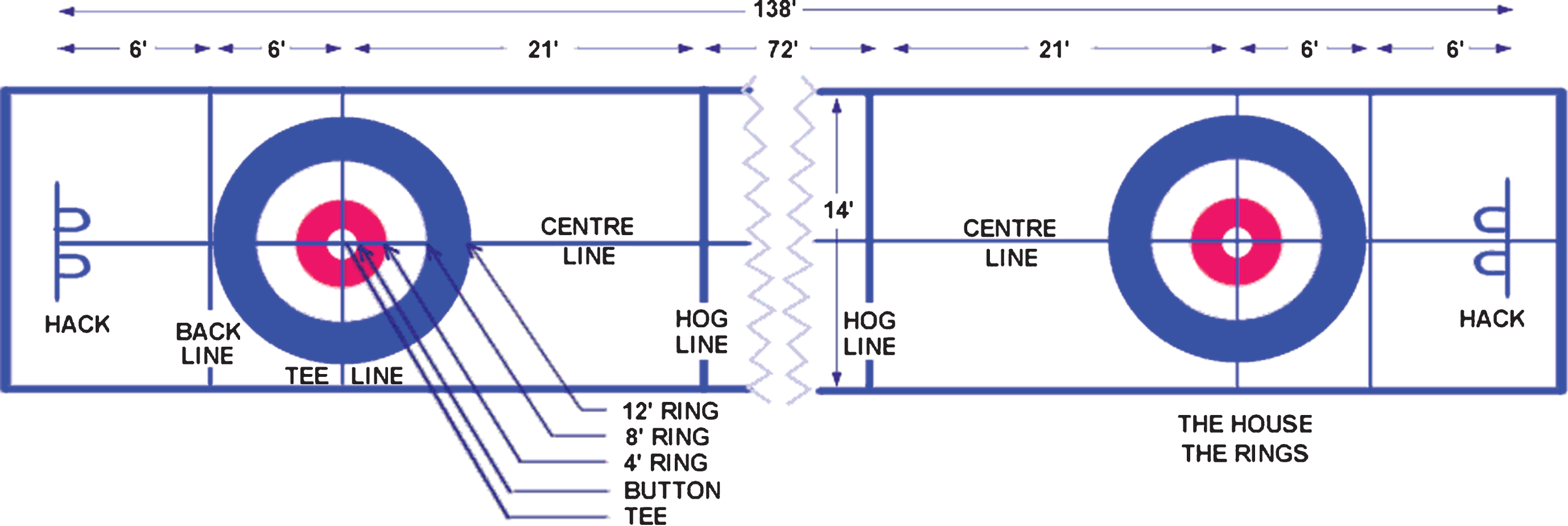
Curling is one of Canada’s most popular sports and has been rising in popularity in the United States since the 2010 and 2014 Winter Olympic Games, as reported by Sports Illustrated (2012) and Carlson (2014). The sport pits two teams against one another in an effort to guide stones down an ice sheet towards the ‘house’ which contains a target known as the ‘button’. Teammates use brooms to sweep the ice in order to influence the movement of the stones in the desired direction. Matches contain ten ‘ends’; individual sets after which the sheet is cleared. Each team is permitted to throw eight stones per end; the team throwing last is said to ‘hold the hammer’. The team with the stone closest to the button at the conclusion of the end has scored. Points are awarded for each stone which is closer to the button than their opponent’s closest stone. Figure 1 illustrates the layout of a ‘sheet’, including the location of the ‘button’ and the ‘house’.
Teams who hold the hammer relinquish control of the hammer if they score points during an end. They do not forfeit the hammer if their opponents manage to ‘steal’ the end and score despite not throwing last. They also do not lose the hammer if no one scores (a ‘blank’ end). It is an assumption among competitors at the highest levels of curling that teams with the hammer can score at least one point during an end, however, many teams choose to strategically blank the end and maintain the hammer rather than take one point but lose hammer control.
Each team is timed; teams currently have a total of 38 minutes per match (40 minutes from 2012-14) to discuss their shots (Curling Canada, 2016). This is a change from the previous timing rule, under which teams had a total of 73 minutes to both discuss their shots and throw their stones (Karrys, 2012). Once a team has run out of time it may no longer throw. Matches may be conceded at any time by either team; the culture of the sport encourages teams which feel they have no chance of winning to concede rather than prolong a decided game.
Given curling’s recent increase in popularity, as well as the relative lack of research into applications of Markov states in the sport, we believe the ability to estimate win probabilities for all given states in curling unlocks a new analysis regime which could materially impact curling decisions and strategy. Empirical win probabilities are not sufficient for understanding state win probability as comeback win likelihood is censored by concession behavior which will be discussed further in the analysis.
Researchers have applied state space models to a wide range of other sports: Baumer, Jensen, and Matthews (2015) applied it to baseball, Koopmeiners (2012) applied it to American football, and Kaplan, Mongeon, and Ryan (2014) applied it to ice hockey. Researchers have also looked at sports outside the “big four” in the United States: Nadimpalli and Hasenbein (2013) examined tennis, and Jarvandi, et al. (2013) used a semi-Markov decision process to examine soccer.
Prior research by Willoughby et al. (2001) modeled curling as a Markov process to find an ‘expected point differential’ at each end. We propose to expand on this analysis by estimating win probabilities of different states in a curling match. These states are defined as a function of end, hammer possession, and score differential, with the probability mass function of scoring being used to define the probability of transitioning between different states. Willoughby and Kostuk (2006, 2005 and 2001) also researched what teams should do with the hammer in the 9th end, finding that it is always better to blank the 9th to keep the hammer. We are curious to see if our model will come to the same conclusion. Finally, Park and Lee (2013) used statistical regressions to determine the probability of winning based on holding the hammer. They found that the most important end to hold the hammer is the 9th.
We created both a three-dimensional empirical state space model and a three-dimensional Markov model in order to analyze win probabilities and answer the following questions: First, what does the Markov model say about win probabilities in the various states and how does the empirical win probability model compare to a Markov model? Next, how can we use these win probabilities to help decide when a team holding the hammer should choose to blank the end? Finally, when should teams concede, and how does this compare to when teams actually concede?
For the purpose of comparing this analysis to prior work, the two most similar papers include Willoughby et al. (2001) and Willoughby and Kostuk (2005).
The Willoughby and Kostuk (2005) paper analyzes a specific decision point facing curls in the 9th end. The decision tree approach pursued in this paper will produce the same results as a Markov model with the same underlying scoring assumptions, but its use and strategic recommendations are restricted to that one end. Through the application of Markov recursive win probability function, one can extend the same logic recursively back to all states of the game.
The Willoughby et al. (2001) uses a Markov model to generate expected point differentials of all states in the game. However, this Markov model is not used to predict win probabilities, something we, the authors, believe is of more relevance given its implications to curling decisions. Curlers shouldn’t care what their expected score differential is, but rather what the likelihood that their score differential is greater than zero by the end of the match for any state of the game, as that is the win condition.
The recursive win probability function (equations 4 & 5) is the novel concept introduced which allows one to solve for all state win probabilities simultaneously with some assumption of underlying scoring distributions and boundary conditions. The cross-state win probabilities unlocks the ability to extend curling strategy recommendations, such as blank versus score, or analyze concession behavior for all possible states of the game.
2Methodology
2.1Data overview
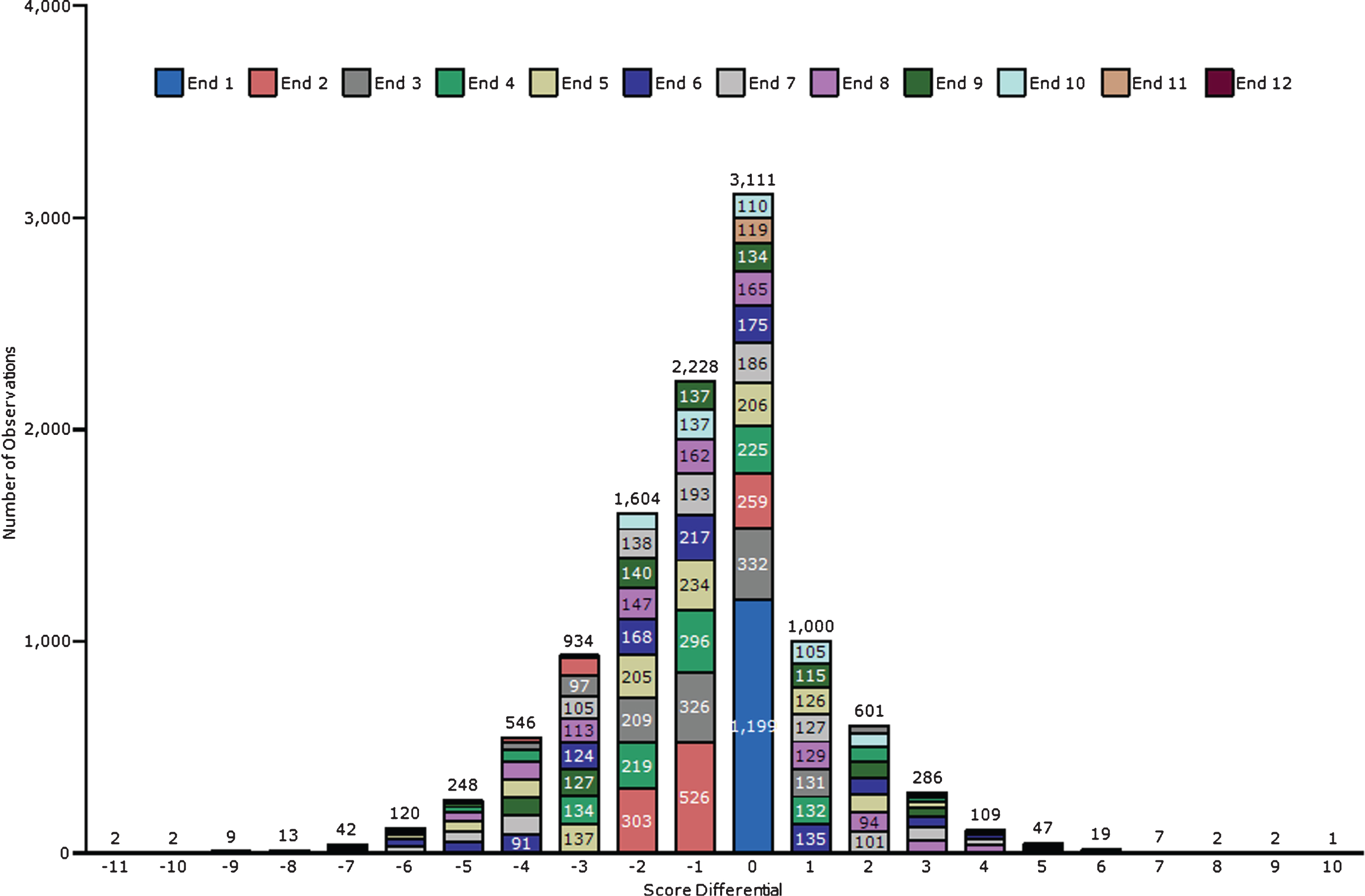
We analyzed matches played in the Canadian Men’s Curling Championships (known for sponsorship reasons as the Labatt Brier, Nokia Brier, or Tim Hortons Brier) from 1998 to 2014. We restricted our analysis to the post-Olympics curling era; curling was first played at the Olympic Games in 1998. We believe that the addition of curling to the Olympics improved the quality of play (World Curling Federation, 2016) and, therefore, did not see value in comparing different eras of the sport. Box score information was retrieved from the Cassidys’ Curling Canada Stats Archive (Cassidy and Cassidy, 2015). The score information included the year of the match, round of the tournament, match location, teams competing, score in each end, final score, time remaining for each team, and which team started with the hammer in the first end. We used information from 10,933 ends reflecting 1,199 matches. Figure 2 summarizes all observed ends by end number and score differential.
Fig.2
Summary of Dataset, Showing Total Observed Ends by Score Differential and End.
We used these data to create a three-dimensional empirical state space tracking three variables. The empirical state space win probabilities were calculated from the frequencies of eventual victories given all observed games in a given state. We also built a three-dimensional Markov model to predict win probabilities assuming a homogeneous scoring distribution. The three state variables used in the models are the end, hammer state and score differential. Table 1 summarizes and explains each state variable.
Table 1
Discrete variables used in three-dimensional state space models
| Variable Name | Range | Description |
| Score Differential | -11 ≤ x ≤ 10 | Reference team’s score less opposing team’s score |
| End | 1 ≤ e ≤ 11 | Beginning of end e |
| Hammer | h ∈{0, 1} | 0: Reference team does not hold the hammer; 1: holds the hammer |
2.2State space overview
To use Markov methodology to model the sport of curling, one must define all possible scenarios that could occur over the course of a game. All permutations from all possible variable values (shown in Table 2) collectively form the state space of the model, where each permutation is a possible state. For example, a particular state may be that the team in question is: down by 2 in the 8th end, and holds the hammer. That state can be represented as (x,e,h) = (–2, 8, 1). The objective of this analysis is to define the eventual win probability of all states in the relevant state space.
Table 2
State space boundary conditions for state space Markov model
| Assumption | Description |
| wp (x ≥ k, e, h) =1 | Team expected to win with certainty once a lead of at least k |
| wp (x ≤ - k, e, h) =0 | Team expected to lose with certainty once trailing by k points |
| wp (x > 0, 11, h) =1 | Team wins if it has a positive score differential after 10 ends (beginning of the 11th end) |
| wp (x < 0, 11, h) =0 | Team loses if it has a negative score differential after 10 ends (beginning of the 11th end) |
| wp (0, 11, 1) | Win probability with hammer advantage after 10th end (see geometric series below) |
| wp (0, 11, 0) | Win probability without hammer advantage after 10th end |
Due to the rules of curling, the possible transitions from each state to the next state are limited. The end of a state must always be greater than the end of a prior state by a value of 1. In other words, ends proceed sequentially throughout the game. Likewise, the hammer possession transitions are defined by the rules of curling, where the hammer possession of a state depends on whether that team held the hammer in the prior state and the end score recorded in that state. Finally, the score differential of a given state is equal to the score differential of the previous state plus the end score.
In order to use a Markov model to exhaustively estimate the win probability of every state in the state space, one must also know all possible state transitions and their associated probabilities. In curling this is simply all possible scores than can be recorded in a single end. From the data it is clear that the likelihood of scoring very much depends on whether a team has the last shot advantage (holding the hammer). The homogeneous model introduced assumes that state transitions are only a function of hammer possession and are thus independent of other parameters in the game such as end or score differential. The heterogeneous model later introduced assumes there is state dependence on the transition function; specifically, that teams play differently based on their current circumstances other than hammer possession. State dependence of the transition function becomes increasingly important in the 10th end, where the team with the higher score at the conclusion of the end wins.
For an example of this state dependence, one would assume that a team down by 2, in the 10th end with hammer advantage would play very differently than a team tied in the 1st end with hammer advantage. The difference in strategy and playstyle is not accounted for in the homogeneous model, but is accounted for in the heterogeneous model.
2.3Empirical state space methodology
With the data prepared, the first step in investigating the state space model required looking at empirical win percentages as a function of the variables described above. The total number of matches that passed through each discrete state were counted, as well as the eventual victors of those matches. The win probability was estimated as the total number of victors over the total number of matches that passed through a particular state.
2.4Markov methodology
The Markov model aims to develop the expected win probability of any curling team given the current state and all potential future transition states. The expected win probability for any state is denoted as: wp (x, e, h) where x is the score differential at the conclusion of end e and h equals 1 if the team holds the hammer.
2.4.1Boundary conditions
To simplify analysis, the boundary conditions summarized in Table 2 are used.
2.4.2Transition to subsequent states
In our analysis, we restricted the number of points scored in a given end to 5 or fewer. Based on empirical data, greater than 5 points are scored in fewer than 0.5% of ends played. Letting y denote change in score during an end, the list of possible transitions from a given state are:
(1)
(2)
That is, from any given end, score and hammer state combination, the following transitions can occur:
• The team scores and will not possess the hammer in the subsequent end
• The end is blanked and hammer possession will not change in the subsequent end
• The team is scored upon and will possess the hammer in the subsequent end
2.4.3Probability of each transition
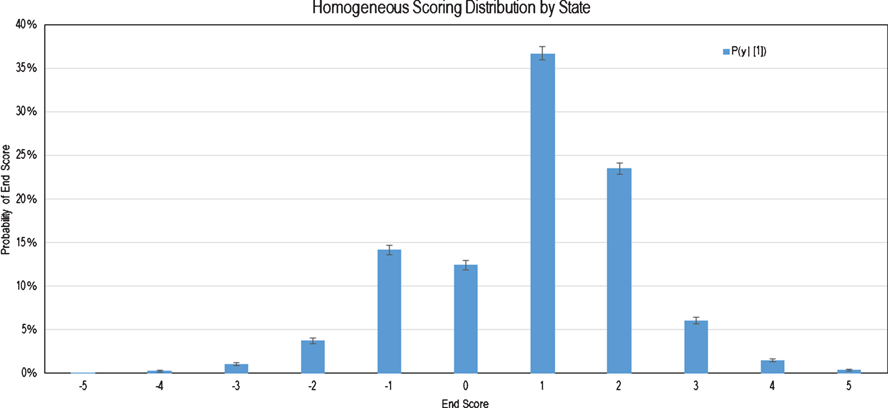
The probability of transitioning from a given state to any one of the possible subsequent states is estimated from empirical scoring distributions conditional on hammer possession. Let P (y|h) denote the conditional probability that a team scores y points given the hammer state h. Because the scoring probability is only dependent on the hammer possession condition, this will be defined as the homogeneous scoring distribution. A summary of the scoring distribution conditional on hammer possession is visualized below.
Later models will incorporate additional conditional information into the transition probability. Let P (y|x, e, h) be the probability of a scoring transition, conditional on the current state of the game as defined by the current score differential, end and hammer possession. This will henceforth be defined as the heterogeneous scoring probability.
However, it is expected that the shooting strategy will be similar across different groups of states. Therefore, some states were grouped together for the purpose of drawing from a common scoring distribution. Specifically, groupings were chosen so that unique scoring probability functions could not be further distinguished within the grouping, but were observed to vary substantially across groupings, due to similar strategy for states within a grouping. The groupings considered for the heterogeneous model are as follows.
• End 1, tie game
• Ends 2–9, all score differentials
• Ends 10–11, individual score differentials
∘ Each score differential represents its own groupings, given how proximate win conditions affect observed shooting strategy
∘ Sub-groupings include ≤ –3, –2, –1, 0, 1, 2, ≥3. As observations for P (y||x|>3, e ≥ 10, h) were unavailable, it was assumed that P (y||x|>3, e ≥ 10, h) = P (y||x|=3, e ≥ 10, h)
This segmentation yields a total of 9 different groups. To populate the scoring distributions of each grouping, all 10,933 ends were segregated and categorized to one of the 9 groupings. A scoring distribution for each grouping would then be generated with the model referencing the appropriate scoring distribution given the state in question.
The complete visualization of all scoring distributions can be found in Fig. 12 in the appendix. As seen in both the homogeneous and heterogenous scoring models, there is a heavy spike at “End score = +1”. This can be explained by curling scoring rules and the fact that each team competing in the Brier is highly skilled. Recall that the winning team at the conclusion of an end is the one whose stone is closest to the center of the target. Furthermore, the winner of each end is awarded points equal to the number of its own stones that are closer to the center than the closest stone placed by its opponent. Thus, assuming that teams competing in the Brier are (roughly) equally and highly skilled, one can imagine the likely outcome of an end being teams alternately placing their stone closer to the center with each throw. The team throwing last (hammer advantage) then places its final stone closest to the center of the target, thereby winning the end and scoring a singular point.
2.4.4Boundary conditions/sensitivity analysis
Recall in Table 2 that a team is assumed to automatically win when ahead by k points and automatically lose when down by k points. In order to determine which boundary condition k to use for the model, one can recalculate the model assuming different values for k.
By incrementally increasing the model parameter k, one can observe the resulting effect on win probability. It is expected that increasing k beyond some threshold will no longer yield substantial changes to Markovian win probabilities. At this point, the model is deemed to have diminished sensitivity to further increases in k, at which point that particular value of k will be used for the final preparation and presentation of the model.
Proper selection of the k parameter allows for a reduction in size of the total Markov state space, thus saving computational effort. The sensitivity analysis allows this selection to be done without sacrificing integrity of the model results.
In practice, concession behavior presents its own boundary for comeback wins, as losing teams tend to concede when they believe the chances of winning are sufficiently low. However, the intention of the Markov model is to predict win probability assuming teams played to completion, so it is not within the scope of the Markov model to incorporate concession behavior. Concession behavior is further analyzed in the results and analysis section by comparing to observed concessions and the associated state specific Markovian win probability.
2.4.5Symmetry
It is important to note an important concept regarding the likelihood of winning and scoring. Due to the nature of the game, the win probability of both the hammer team and the non-hammer team must sum to 1 for any given state of the game.
Likewise, the scoring probability of the non-hammer team is exactly the opposite of the hammer team. For any given state, the probability of the non-hammer team to score y points in an end must be the same as the hammer team scoring – y, with their respective score differentials reversed.
Mathematically, the concept of symmetry with regards to win probability can be represented as the following: wp (x, e, 0) = 1 - wp (- x, e, 1).
Likewise, symmetry for scoring probability can be represented as the following: P (y|x, e, 0) = P (- y| - x, e, 1).
Because symmetry allows us to easily estimate the probabilities associated with non-hammer states given estimated probabilities from hammer states, tables and figures in this work will only present probabilities from the perspective of the hammer team.
2.4.6Estimating win probability in extra ends
If two teams are tied at the conclusion of 10 ends, extra ends are played. In the 11th end, there are two possible outcomes: one of the teams scores one or more points and wins the match, or the end is blanked and the match continues for a 12th end. By analogy, the possible outcomes for the 12th and subsequent ends are the same.
Thus, the win probability for the team holding the hammer in extra ends is:
(3)
Because the strategy shouldn’t change in either “next score wins” situation, we can assume the probability distribution of scoring will be the same for all ends after the 10th when the score is tied. With that assumption, it can be inferred that the probability of the team with the hammer winning in extra ends is the sum of the resulting geometric sequence. From Fig. 3, P(y ≥ 1|1) = 68.23 % (the probability the hammer team scores one or more points in a given end) and P(y = 0|1) = 12.42 % (the probability of a blank end given hammer possession).
Fig.3
Homogeneous Probability Mass Function of Scoring.
Subsequently, we can calculate
Likewise, the same logic can be used to estimate the heterogeneous win probability wp(0,10,1). From Fig. 4, P(y ≥ 1|0, 10, 1) = 79.97 % and P(y = 0|0, 10, 1) = 0 %.
Fig.4
Heterogeneous Probability Mass Function of Scoring of Select Groupings.
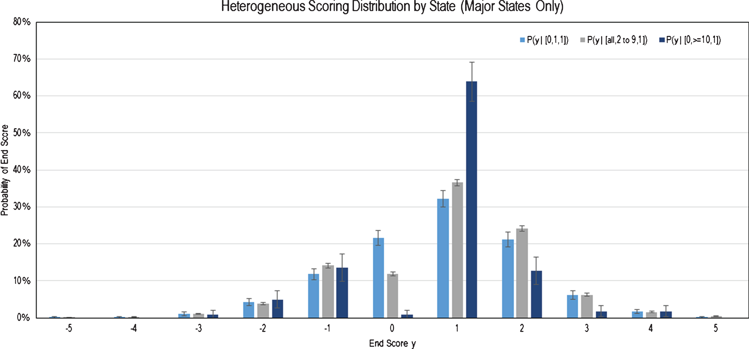
Subsequently, we can calculate
2.4.7Transition equation
The Markovian win probability of a given state can be calculated as the probability-weighted average of win probabilities associated with all homogeneous possible state transitions j:
(4)
Likewise, the Markovian win probability of any given state can be calculated using heterogeneous state transitions j:
(5)
2.4.8Uncertainty analysis
To estimate the uncertainty associated with the win probabilities predicted by the Markov model, bootstrapping can be performed using random resampling and replacement. The resulting variability in scoring probabilities and Markovian win probabilities indicates the uncertainty.
Specifically, each end in the dataset was substituted with a randomly drawn end. The randomly drawn end is generated by randomly selecting one of the 10,933 ends, recording the end score and associated state, and repeating 10,933 times to generate a new dataset. For that iteration, the new resampled dataset would create a scoring distribution from which a new Markov model could be generated with win probabilities for each state. After 10,000 iterations, estimates of the uncertainty associated with each scoring probability and win probability were generated from the resulting distribution.
This procedure was applied for both the homogeneous and heterogeneous models. It can be predicted that the large dataset would yield low uncertainty for the homogeneous model, as the probability of scoring y points is built from a distribution reflecting all 10,933 ends and thus not expected to vary with resampling from such a large common distribution. However, the heterogeneous model contains state specific scoring distributions, thus necessitating isolation of different groups of states as described earlier. This segregation yields smaller sub-datasets supporting the scoring distribution for that grouping of states, contributing to higher uncertainty for grouping in which fewer ends were observed. Because each of the 10th end state scoring distributions were segregated into separate groups, the uncertainty associated with win probabilities in the 10th end is expected to be high, thus reflecting the smaller supporting dataset.
3Results & analysis
3.1Sensitivity analysis results
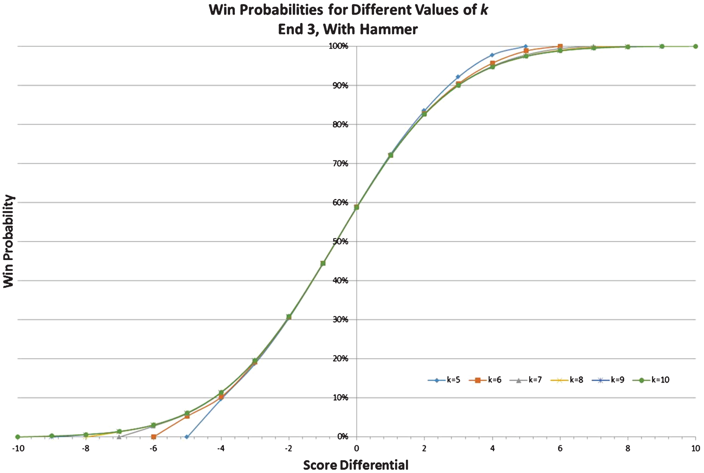
Before the model was finalized, a decision regarding model parameter k was required. Recall from Table 2 that parameter k represents the boundary condition for score differential at which the outcome of the game is assumed to be a foregone conclusion. As described earlier, Markovian win probabilities exhibit diminishing sensitivity to k. Multiple versions of the homogeneous Markov model were calculated and presented in Fig. 5 for 5 ≤ k ≤ 10.
Fig.5
Win Probabilities for Given States Assuming Different Model Parameters k.
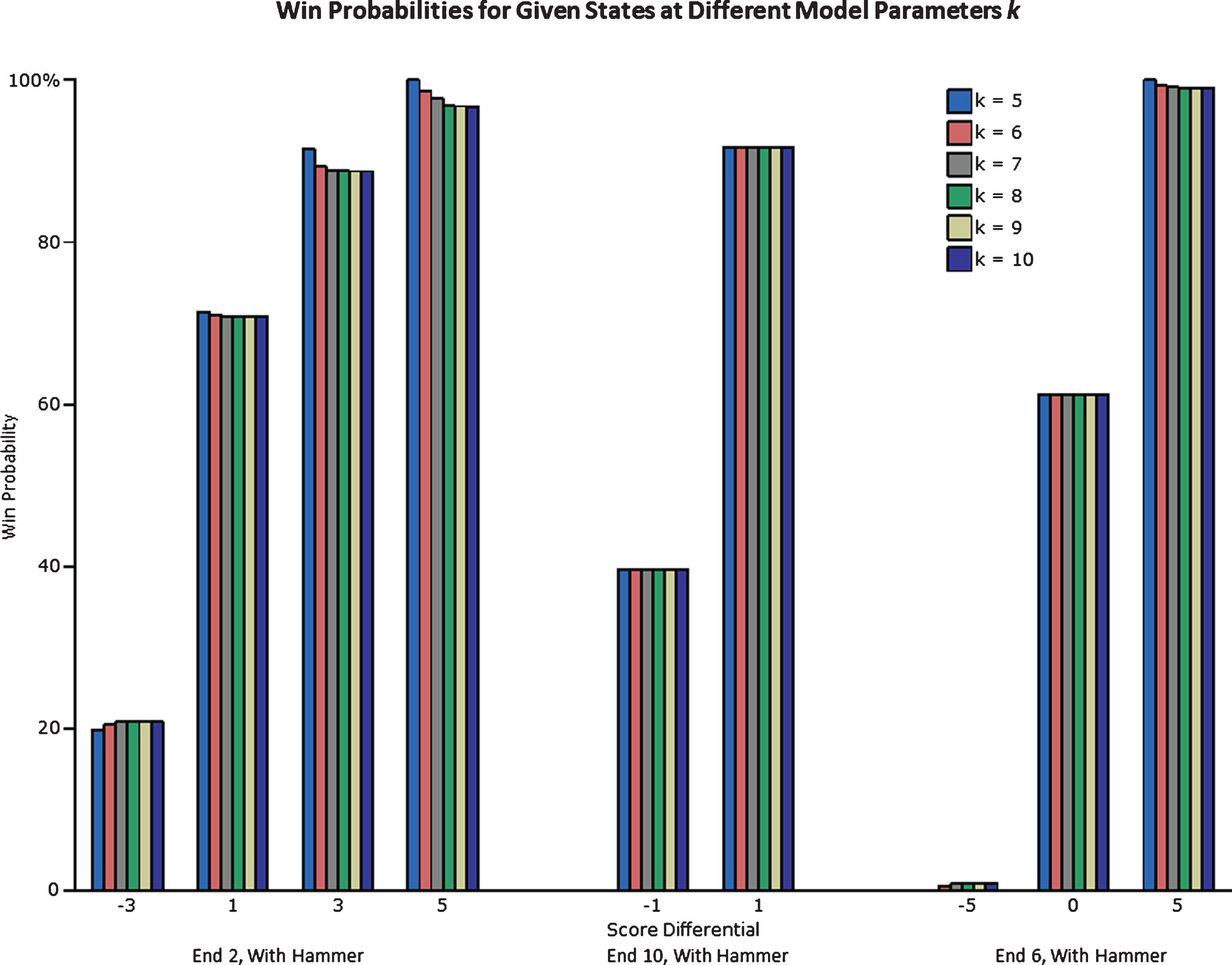
As can be observed, most win probabilities are not sensitive to k across all model iterations. States which were the most sensitive to k include those early in the game and with lopsided score differentials.
Because all state specific win probabilities stabilized at k ≥ 8, it was concluded that this value would be sufficient and was thus selected for further analysis.
An alternative visualization of model sensitivity to k is presented in the appendix in Fig. 13.
3.2Empirical win probability
Before modelling win expectations, the likelihood of any team winning the match in any given state was estimated directly from the dataset. This was done by isolating all score differential and end combinations separately and tracking whether the hammer team in that scenario emerges as the eventual victor. The fraction of all observations in which the hammer team eventually wins is considered the empirical win probability for that state. The results are summarized in Table 3. While Table 3 describes the fraction of eventual victors for any given state, it does not count the total number of observations for each state. Blanks cells indicate no observations and thus, the empirical win probability could not be estimated.
Table 3
Empirical win probabilities at the beginning of each end with hammer advantage
| Beginning of End | Point Differential | |||||||||||||||||||||
| –11 | –10 | –9 | –8 | –7 | –6 | –5 | –4 | –3 | –2 | –1 | 0 | 1 | 2 | 3 | 4 | 5 | 6 | 7 | 8 | 9 | 10 | |
| 1 | 59% | |||||||||||||||||||||
| 2 | 0% | 0% | 5% | 12% | 28% | 41% | 60% | |||||||||||||||
| 3 | 0% | 0% | 0% | 0% | 13% | 8% | 23% | 47% | 62% | 82% | 91% | 100% | 100% | |||||||||
| 4 | 0% | 0% | 0% | 0% | 0% | 4% | 10% | 22% | 45% | 64% | 78% | 91% | 95% | 100% | 100% | 100% | ||||||
| 5 | 0% | 0% | 0% | 0% | 0% | 0% | 0% | 2% | 9% | 20% | 48% | 55% | 80% | 94% | 100% | 100% | 100% | 100% | 100% | 100% | ||
| 6 | 0% | 0% | 0% | 0% | 0% | 0% | 3% | 6% | 27% | 41% | 65% | 85% | 91% | 100% | 100% | 100% | 100% | 100% | 100% | 100% | ||
| 7 | 0% | 0% | 0% | 0% | 0% | 0% | 10% | 17% | 36% | 66% | 83% | 95% | 100% | 100% | 100% | 100% | 100% | 100% | 100% | |||
| 8 | 0% | 0% | 2% | 1% | 6% | 22% | 41% | 64% | 94% | 98% | 100% | 100% | 100% | 100% | 100% | |||||||
| 9 | 0% | 0% | 0% | 1% | 10% | 36% | 63% | 86% | 100% | 100% | 100% | 100% | ||||||||||
| 10 | 18% | 24% | 44% | 83% | 95% | 100% | 100% | |||||||||||||||
| 11 | 78% | |||||||||||||||||||||
| 12 | 100% | |||||||||||||||||||||
3.3Markov model results
1. What does the Markov model say about win probabilities in the various states? How does the empirical win probability model compare to a Markov model?
Figure 6 below illustrates the results of the homogeneous Markov model (solid lines) against those of the empirical model (discrete points). The legend indicates the score differential, while the horizontal axis indicates the end in question. All win probabilities are presented from the perspective of the hammer team. Following a single line to the right would be the equivalent of tracking the Markov win probability of a team consistently blanking ends as the game approached its conclusion.
Fig.6
Homogeneous Markovian Win Probabilities at the Conclusion of Each End with Hammer Advantage (Modeled vs. Observed).
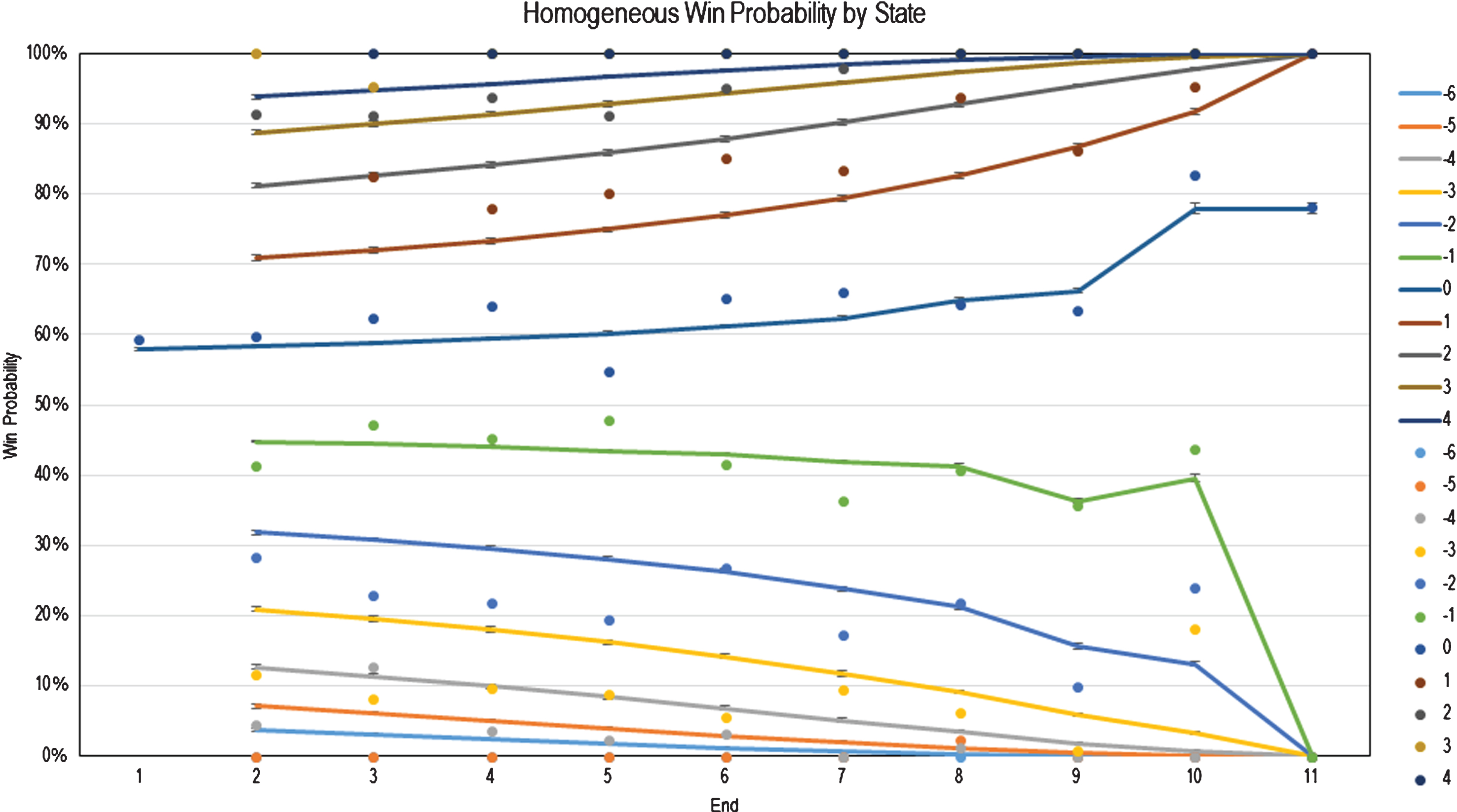
One insight from the homogeneous model is that it pays to start the match with the hammer: teams that hold the hammer at the beginning of a match have a 58% chance of winning. This result is consistent with the results reported by Park and Lee (2013) as well as Willoughby et al. (2001).
Although the homogeneous model generally reports the same win probability trends as the empirical model when the match is close, it consistently over-predicts the likelihood of comebacks compared to actual match data.
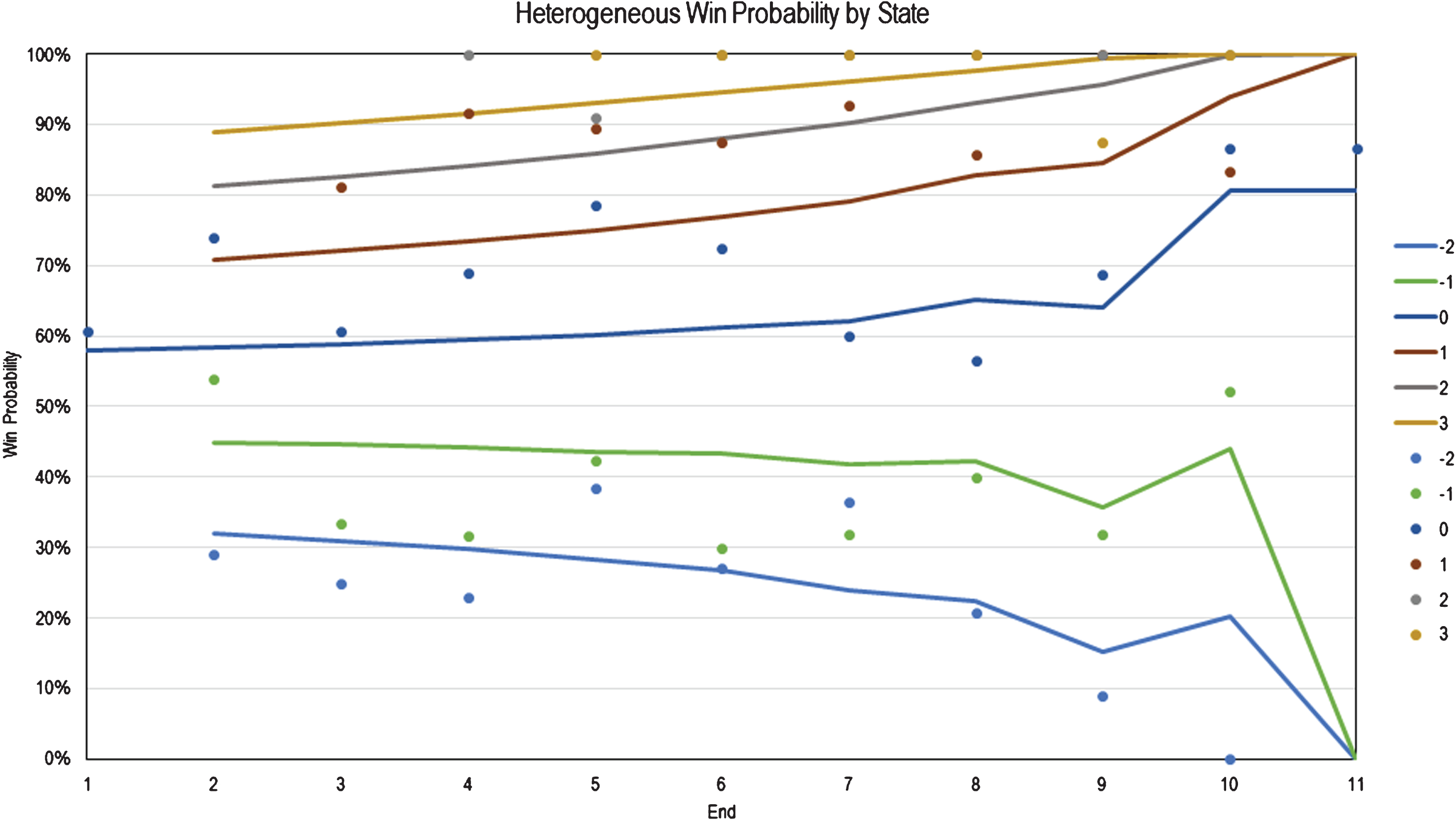
We subsequently extended our Markov analysis by incorporating a state specific scoring distribution that varied by end to arrive at the heterogeneous Markov Model. Figure 7 below plots the results of this new heterogeneous model (solid lines) against those of the empirical model (discrete points). The results of the heterogeneous model are largely consistent with those of the homogeneous model, with improved fit observed later in the match (e.g. for the 10th end). This is due to the fact that the heterogeneous scoring distribution aims to take into account the state-dependence of the scoring distribution, which becomes especially relevant in the 10th end due to proximate win conditions. For example, the shooting strategy of a team down by 2 with the hammer in the 10th end can be expected to be very different from that of the same team up by 1. Segregating and filtering the data set across these states yields different observed probabilities of scoring.
Fig.7
Heterogeneous Markovian Win Probabilities at the Beginning of Each End with Hammer Advantage.
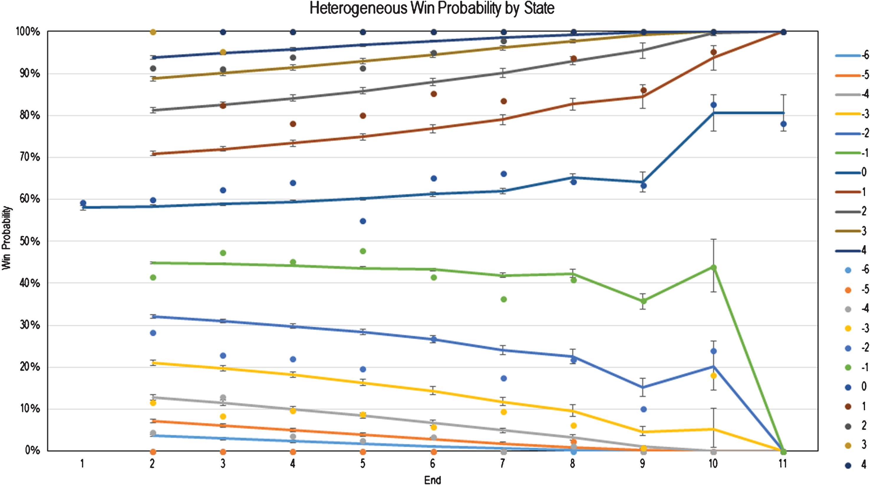
In general, teams appear to play more defensively when ahead in later ends of a match, which reduces the likelihood of late-game comebacks. This is perhaps unsurprising, as this sort of behavior is common across many sports. It is worth noting, however, that even the heterogeneous model overestimates the likelihood of late comebacks for larger (>2) score differentials. A possible explanation for this over-prediction is that the heterogeneous model’s score distribution is not dependent on score differential until the 10th end or later, thus defensive behavior is not captured fully before the 10th end.
The results of both Markov models, in addition to empirical win probabilities, agree with the conclusions made by Kostuk and Willoughby (2004) who determined that it is preferable to go into the 10th end up by one without the hammer rather than down by one with the hammer assuming the probability of scoring one or more points with the hammer is greater than 0.5. Our scoring probability mass function estimates a 68% chance of scoring one or more points in an end when holding the hammer; our heterogeneous Markov model shows the win probability is 56% entering the 10th end up by one without the hammer and 44% when entering the 10th end down by one with the hammer.
Regarding the lower modelled likelihood of a comeback versus empirical results, we offer the following hypotheses to help explain the difference.
a. Conceding a match is a practice considered polite once a team realizes that the probability of winning a match is sufficiently low. The empirical data records concession as a loss without recording the possible alternative of a comeback win. This behavior will likely polarize win probabilities (lower in disadvantaged situations, higher in advantaged situations) and lead to the observed discrepancy between the model and the empirical. Essentially, concession behavior in curling censors the dataset and prevents observations in comeback probabilities.
b. The homogeneous model also assumes that the scoring distribution is only a function of hammer possession and does not depend on ends or point differential. From our knowledge of curling strategy, teams generally play defensively when holding the lead. This lowers the variability of scoring, thus lowering the likelihood of a comeback if the strategy is successfully executed. The model does not account for this particular state dependence.
i. Further support for this hypothesis is the fact that the Markov Model assuming a heterogeneous scoring model (which has more granular scoring distribution assumptions for the 10th end) offers a better fit against empirical results for the 10th end vis-á-vis the same model assuming a homogeneous scoring model. This suggests that increasing the state-dependence of our end-to-end scoring assumptions reduces the current overestimating of comebacks and improves overall fit. However, the improved prediction for comeback situations is primarily observed in later ends. The heterogeneous model does not seem to produce better predictions for comebacks in earlier ends. It is likely that the first explanation dominates in these situations as an extreme imbalance in early ends will likely result in a concession, censoring the dataset to prevent observed comebacks.
3.4Model uncertainty
Uncertainty was estimated in the model using standard bootstrapping analysis. Figures 6 and 7 contain error bars which were derived from the distributions accumulated via resampling and replacement. The span of the error bars represents a 95% confidence interval.
Predictably, the homogeneous model exhibits low uncertainty. The large dataset was not segregated as there was no state dependence on the probability of scoring. Thus, all 10,933 ends were resampled to produce new iterative scoring distributions, leading to minimal model variation. The average span of the 95% confidence interval is 0.55% across all states.
The heterogeneous model exhibits higher uncertainty. Because all 10th end states were grouped separately far fewer observations were recorded for each grouping. Therefore, bootstrapping yields higher variability which can be observed by the wider confidence intervals moving into the later ends.
3.5Data validation
We further validated our Markov analysis by plotting the heterogeneous model against empirical win probability implied by 2015 and 2016 Brier Tournament results. These years were not included in the data set used to develop the model: therefore, testing against this additional data would further validate our model. Similar to the section above, Tables 4 and 5 summarize the empirical win probabilities for each state with hammer advantage for the 2015 and 2016 tournament years.
Table 4
Empirical win probabilities at the beginning of each end with hammer advantage for 2015 and 2016 tournaments
| Beginning of End | Point Differential | |||||||||||||||
| –8 | –7 | –6 | –5 | –4 | –3 | –2 | –1 | 0 | 1 | 2 | 3 | 4 | 5 | 6 | 7 | |
| 1 | 61% | |||||||||||||||
| 2 | 50% | 29% | 54% | 74% | ||||||||||||
| 3 | 0% | 0% | 0% | 25% | 33% | 61% | 81% | |||||||||
| 4 | 0% | 0% | 6% | 23% | 32% | 69% | 92% | 100% | 100% | |||||||
| 5 | 0% | 0% | 0% | 0% | 0% | 38% | 42% | 79% | 89% | 91% | 100% | |||||
| 6 | 0% | 0% | 0% | 11% | 27% | 30% | 72% | 88% | 100% | 100% | 100% | 100% | 100% | |||
| 7 | 0% | 0% | 0% | 0% | 0% | 36% | 32% | 60% | 93% | 100% | 100% | 100% | 100% | 100% | ||
| 8 | 0% | 0% | 0% | 6% | 0% | 21% | 40% | 57% | 86% | 100% | 100% | 100% | 100% | 100% | ||
| 9 | 0% | 0% | 0% | 1% | 10% | 36% | 63% | 86% | 100% | 100% | 100% | 100% | ||||
| 10 | 18% | 24% | 44% | 83% | 95% | 100% | 100% | |||||||||
| 11 | 78% | |||||||||||||||
| 12 | 100% | |||||||||||||||
Table 5
Heterogeneous Markov model strategy matrix. Values show the marginal win probability advantage of blanking over scoring 1. Green indicates blanking is the optimal strategy
| Decision End | Point Differential | ||||||||||
| –5 | –4 | –3 | –2 | –1 | 0 | 1 | 2 | 3 | 4 | 5 | |
| 1 | 3.2% | ||||||||||
| 2 | 0.9% | 1.5% | 2.3% | 3.0% | 3.4% | 3.4% | 3.0% | 2.3% | 1.5% | 0.9% | 0.5% |
| 3 | 0.8% | 1.5% | 2.3% | 3.1% | 3.7% | 3.7% | 3.1% | 2.3% | 1.5% | 0.8% | 0.4% |
| 4 | 0.7% | 1.4% | 2.2% | 3.2% | 3.8% | 3.8% | 3.2% | 2.2% | 1.4% | 0.7% | 0.3% |
| 5 | 0.6% | 1.3% | 2.4% | 3.6% | 4.5% | 4.5% | 3.6% | 2.4% | 1.3% | 0.6% | 0.2% |
| 6 | 0.4% | 1.0% | 1.9% | 3.0% | 3.8% | 3.8% | 3.0% | 1.9% | 1.0% | 0.4% | 0.1% |
| 7 | 0.3% | 0.9% | 2.6% | 5.2% | 7.5% | 7.5% | 5.2% | 2.6% | 0.9% | 0.3% | 0.1% |
| 8 | 0.0% | 0.3% | 0.2% | –0.2% | –0.2% | –0.2% | –0.2% | 0.2% | 0.3% | 0.0% | 0.0% |
| 9 | 0.0% | 0.0% | 5.0% | 14.0% | 24.8% | 24.8% | 14.0% | 5.0% | 0.0% | 0.0% | 0.0% |
| 10 | 0.0% | 0.0% | 0.0% | 0.0% | –19.3% | –19.3% | 0.0% | 0.0% | 0.0% | 0.0% | 0.0% |
| 11 | –19.3% | ||||||||||
Table 6
Expected concession behavior given win probability threshold of 2.57% with hammer advantage
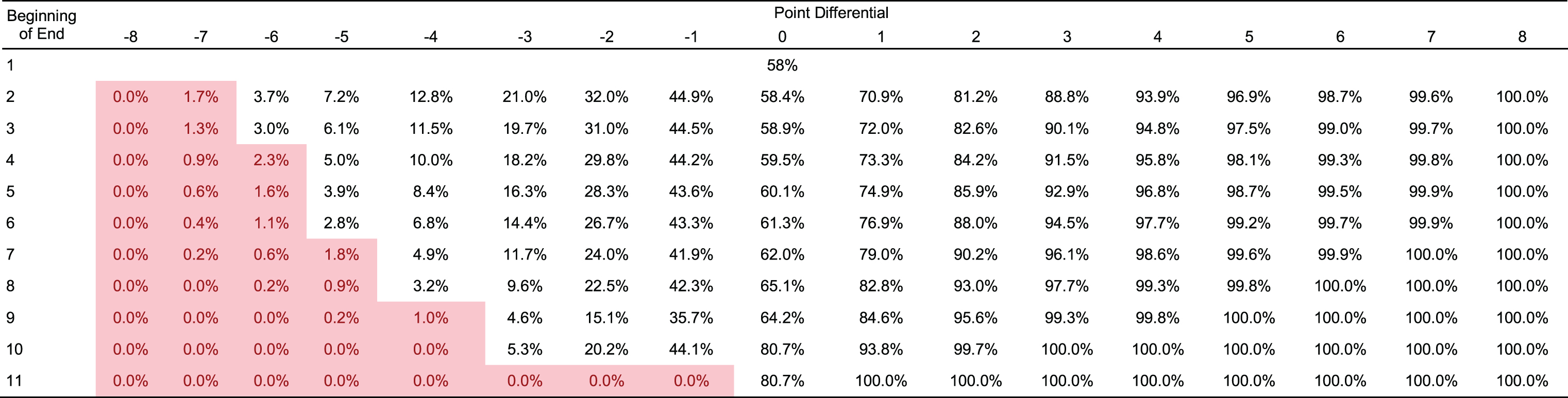 |
Table 7
Expected concession behavior given win probability threshold of 2.57% without hammer advantage
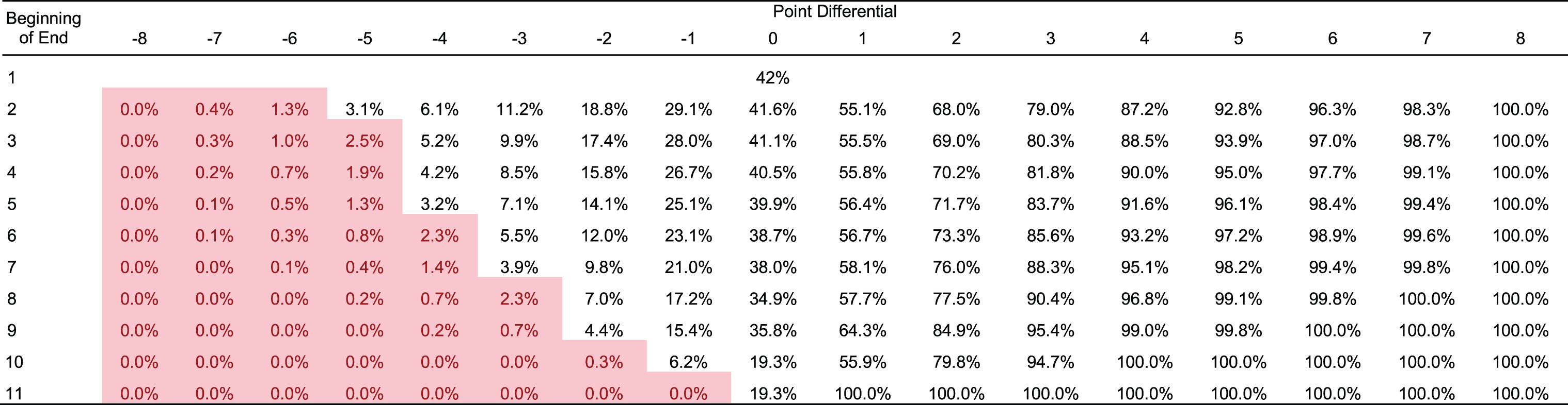 |
Table 8
Observed number of concessions and associated state win probability
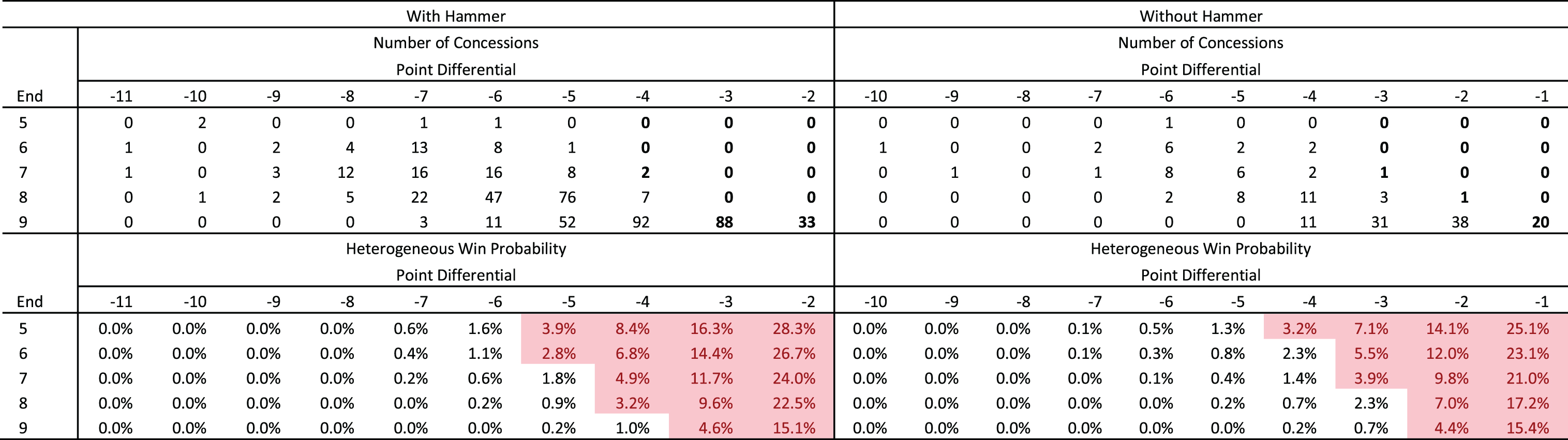 |
Figure 8 below show the results when the heterogeneous Markov Model (solid lines) are plotted against those of the empirical model for the 2015 and 2016 tournaments (discrete points).
Fig.8
Heterogeneous Markovian Win Probabilities at the Conclusion of Each End with Hammer Advantage. Empirical data shown for 2015 and 2016 tournament years (Modelled vs. Observed).
The results of this analysis generally agree with the initial validation in the above section. The heterogeneous model continues to overestimate the likelihood of late comebacks of score differentials greater than 2. The 2015 & 2016 Brier empirical win rates seem to indicate that the model over-estimates the likelihood of a comeback to an even larger extent compared to the 1998–2014 dataset. A possible explanation for this over-estimation is that teams have become more consistent and precise over the years, reducing variability of scoring and thus, reducing likelihood of a comeback. Because the model was derived from scoring probability of the 1998–2014 dataset, the hypothesized reduced variability of scoring in later years wouldn’t reflect in the model. Thus, the model would appear to over-predict comebacks to an even greater degree. This contribution would be cumulative with the aforementioned effect of the concession behavior, where concession behavior would be expected to reduce likelihood of comebacks.
In addition, the heterogeneous model overestimates the likelihood of comebacks during the middle of a match – specifically, between ends 4 and 6. There also appears to be high deviation in the empirical win probabilities around ends 5 and 8: the likelihood of a comeback decreases until the halfway point whereby comebacks become increasing likely until end 8 before decreasing again. This phenomenon is also observed in the initial data set to a lesser degree. This suggest the pronounced inflections in the 2015 and 2016 data may be due to additional noise from a smaller dataset or a peculiarity in these tournament years.
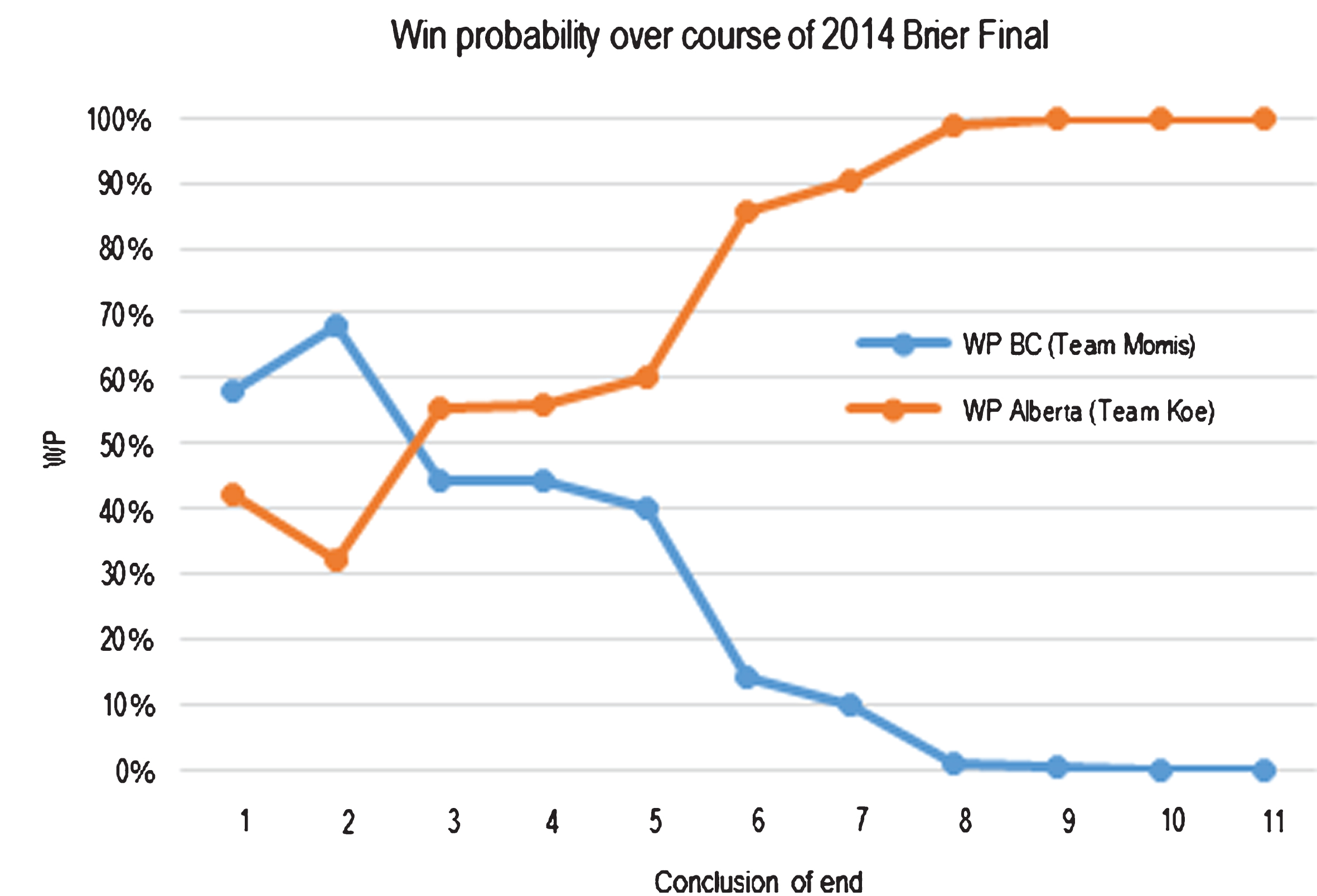
3.6Model implications and use cases
The Markov model allows us to graph the expected win probabilities for each team over the course of a match in a manner similar to those supplied on popular websites for other sports. Figure 9 provides an example of this win probability scoreboard for the championship match of the 2014 Brier between Team BC and Team Alberta.
Fig.9
Sample “Alternative Scoreboard” for the 2014 Brier Tournament Championship Match.
2. How can we use these win probabilities to help decide when a team holding the hammer should choose to blank the end?
We can see that the relative advantage of holding the hammer increases as the conclusion of the match approaches, most starkly at the conclusion of the 9th end. Teams are commonly faced with the following decision: score one point and give up the hammer in the subsequent end or blank the end to retain possession of the hammer in the subsequent end. Looking at win probabilities this decision can be modelled mathematically as:
(6)
If this inequality holds true, the team should choose to blank the end, assuming that teams are sufficiently skilled to blank the end with 100% certainty. Otherwise, the team should take the point, also assuming that the teams are sufficiently skilled to score one point with 100% certainty. If we check this inequality for every possible state of the match using the heterogeneous Markov model, Table 5 is produced.
The analysis indicates that prior to the seventh end, it is always preferable to blank the end, regardless of other factors.
However, there are two broad recommendations that are intriguing at first glance. First, the matrix suggests blanking in the 9th end if down by one or tied, which aligns with the general intuition that it is preferable to retain the hammer in the 10th end for close matches.
In the eighth end, the matrix suggests that it is preferable to score one rather than blank for score differentials between –2 and +1 (inclusive). This recommendation should generally agree with intuition since this will allow the team holding the hammer in the 8th end to regain the hammer for the 10th end in a close match. However, the marginal advantage of scoring one versus blanking in the 8th is minor and within the margin of error presented in the bootstrapping analysis.
Our recommendation for the 9th end is consistent with that of Willoughby and Kostuk (2005), which concludes that it is always preferable to blank in the 9th in order to retain the hammer. Willoughby et al. (2005) assumed an empirical scoring distribution conditional on score differential and end, while our analysis considers either a homogeneous scoring distribution as a function of only hammer possession, or a heterogeneous scoring distribution as a function of end, score differential (for the 10th end only) and hammer possession. The conclusion, however, is the same. Furthermore, the Markov model can use recursive logic to extend the strategy recommendation back to all possible states of the game and finds that this recommendation holds in most cases.
We can further generalize the strategy implications to a hypothetical curling match with infinite ends. In this situation, each team will want to maximize the expected value of their point differential. When a team with the hammer scores, the immediate point(s) associated with that score are realized, but the team loses the value associated with hammer possession. When the non-hammer team is scored upon, that team’s point differential is reduced but is partially compensated for with the benefit of subsequently controlling the hammer. Suppose v is the value of the hammer possession, r is the number of expected points scored per end with hammer possession, and p is the probability of maintaining hammer possession through the next end. We can see that the following equation must hold:
(7)
Solving for v, this reduces to ...
(8)
Assuming the homogeneous scoring probability mass function illustrated in Fig. 3, we can see that:
Therefore, the value of holding the hammer is equal to 0.614.
When considering a situation where the team with hammer possession is deciding between shooting aggressively or blanking the end with complete certainty, then the following inequality must hold true to justify scoring over blanking an end:
(9)
We can see that given the value of the hammer of 0.614 points, the aggressive strategy must yield at least 1.23 points on average to be justified, or two points in practice. If the decision involves blanking versus scoring one point, blanking is always the optimal strategy in infinite curling, which is consistent with the recommendations presented in Table 5 for finite curling (with some minor exceptions).
3. When should teams concede? How does this compare to when teams actually concede in real life?
The heterogeneous Markov model assumes that a team has zero chance of winning if the deficit reaches eight points, with this assumption being supported by the sensitivity analysis presented earlier. Implicit in this assumption is the expectation that the teams play out regardless of either team’s win probability. However, concession behavior censors observed win likelihood in high point differential situations. None of the major authorities including the World Curling Federation, the U.S. Curling Association, and the Canadian Curling Association, have strict guidelines on when teams should concede.
To answer the first question we assume that there exists a threshold, w* such that if a team’s win probability dips below this threshold, the team should concede the match per curling etiquette. Summarizing all conceded matches in the 1998–2014 Brier Tournaments, we arrive at Figs. 10 and 11 illustrating the frequency of concessions by win probability at time of concession.
Fig.10
Observed number of concessions against conceding team’s win probability at time of concession when conceding team holds the hammer.
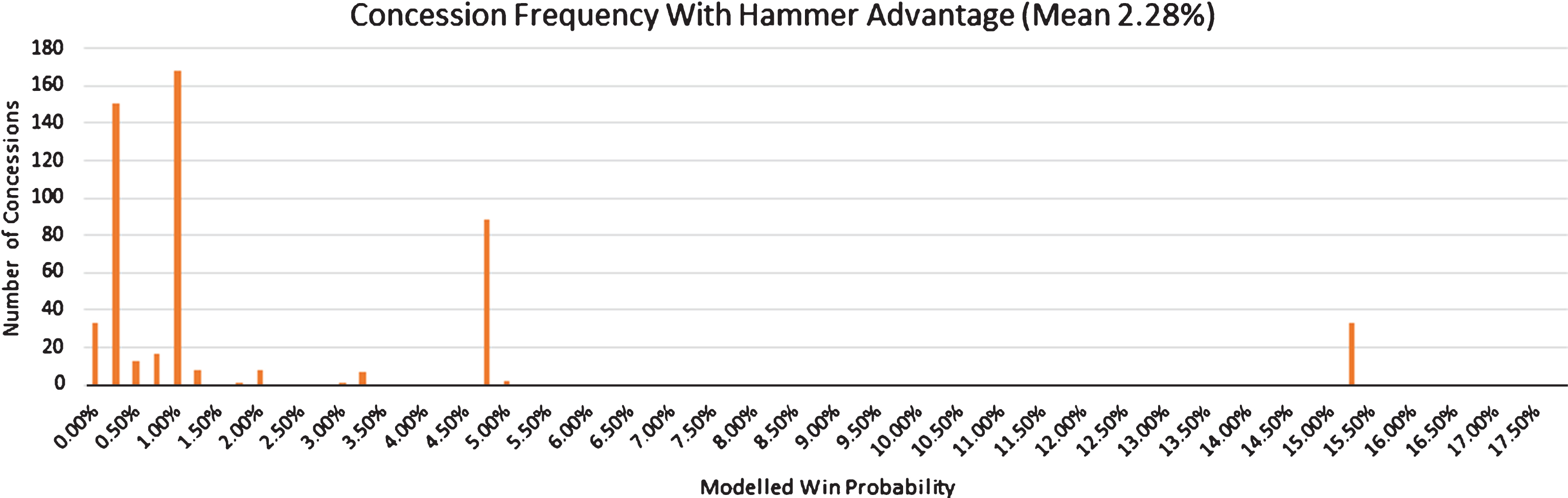
Fig.11
Observed number of concessions against conceding team’s win probability at time of concession when conceding team does not hold the hammer.
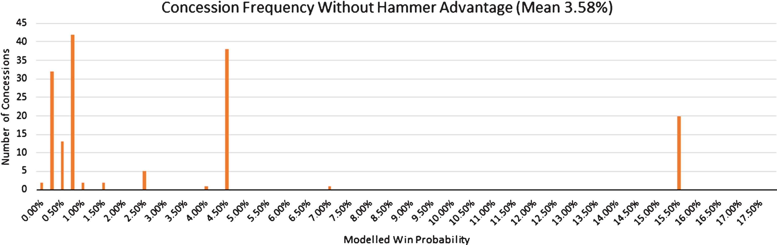
Intuitively, teams are observed conceding when their win probability is sufficiently low, with the mean win probability at time of concession being 2.28% when the team possessed the hammer and 3.58% when the team did not possess the hammer. Therefore, it appears that most teams have a psychological threshold for w* of around 2.57% averaged across both situations. Given this value of w* and the Markovian win probabilities, Tables 6 and 7 illustrate states in the game where one would expect to see the losing team concede.
This is compared to the observed concessions and the implied Markov win probabilities at the time of concession as represented in Table 8.
As illustrated, teams do not appear to concede above the 2.57% average threshold with the notable exception of the 9th end, where there were 53 observed concessions in a state where the win probability was above 15%, and 88 observed concessions with a win probability of 4%. Furthermore, teams who held the hammer but were down two points after the 9th end conceded 33 times, even though they still had a 15% chance of winning the match!
These exceptions may be partially explained by the fact that the Markov model currently does not take the clock into account. Prior to 2012, teams had 73 minutes to make all of their shots in a game. From 2012 forward, this rule was modified to provide teams with 38 minutes of “thinking time”. As the data did not differentiate situations where the clock had expired, these observations were not excluded. The win probability in a state where the team’s clock is near expired is likely lower than the probability predicted by the model thus, many of the concessions may still have been made adhering to the 2.57% average threshold mentioned earlier.
In addition, the win probability at time of concession only accounts for the win probability assuming the concession occurs before any stones are thrown. However, it is possible for a team to concede in the middle of the end, at which time they have a better assessment of the situation given additional conditional information which could affect win probability. For example, a team down by two, with the hammer, in the beginning of the 9th end is considered to have a win probability of 15%. However, if that end is proceeding poorly for that team, they may accurately assess that their win probability has decreased below 15%. If that team concedes before the end is concluded, no score will be posted and that game will appear to have ended before any stones were thrown in the 9th end.
In this situation, the modelled win probability will not incorporate the change in the situation which occurred during that incomplete end. Therefore, the team making the decision may have more information than what is available in the data, thus the analysis likely overestimates win probability at time of concession.
3.7Summary
In this study we used 18 years of tournament data from the Canadian Men’s Curling Championships to develop empirical as well as homogeneous and heterogeneous Markov models to analyze win probabilities in curling.
Both the homogeneous and heterogeneous Markov models suggest a lower likelihood of comeback versus empirical results, with a possible explanation being that concession behavior censors potential comeback wins, thus biasing observations towards fewer comebacks.
The heterogeneous model improves on the homogeneous model with a better fit line for states at later ends, due to state-specific scoring probabilities diverging from the average towards the end of the game as the proximate win conditions alter the optimal shooting strategy. However, larger uncertainty is also observed in the heterogeneous model, as fewer state-specific observations yield greater variability in the bootstrapping analysis.
The results of the models have afforded us new insights that can be applied to curling strategy. For example, when presented with the choice to score one point or blank the end, teams should always blank the end regardless of situation, prior to the 7th end. However, teams should only blank the 8th for score differentials between –2 and 1 (inclusive), and should attempt to score for other score differentials in the 8th end. Finally, if we assume that teams have a psychological concession threshold of a 2.57% win probability, our analysis would indicate that teams concede matches more frequently than they should, which could encourage teams to continue to play out matches they currently concede.
In addition, the win probability changes presented in table 5 allow one to formally evaluate the “blank vs score 1” strategic question. With minor exceptions, it is always favorable to blank in the first 9 ends. This largely agrees with the quantitative analysis of curling available in other literature. However, the degree of favorability depends on the state of the game, with the 8th end representing the exception where blanking isn’t expected to yield an advantage compared to the alternative strategy of scoring 1.
In general, extending the Markov analysis to all possible states yields interesting insights and allows for a more rigorous analysis of curling behavior and strategy.
Appendices
Appendix
Fig.12
All Heterogeneous Scoring Probabilities by Grouping.
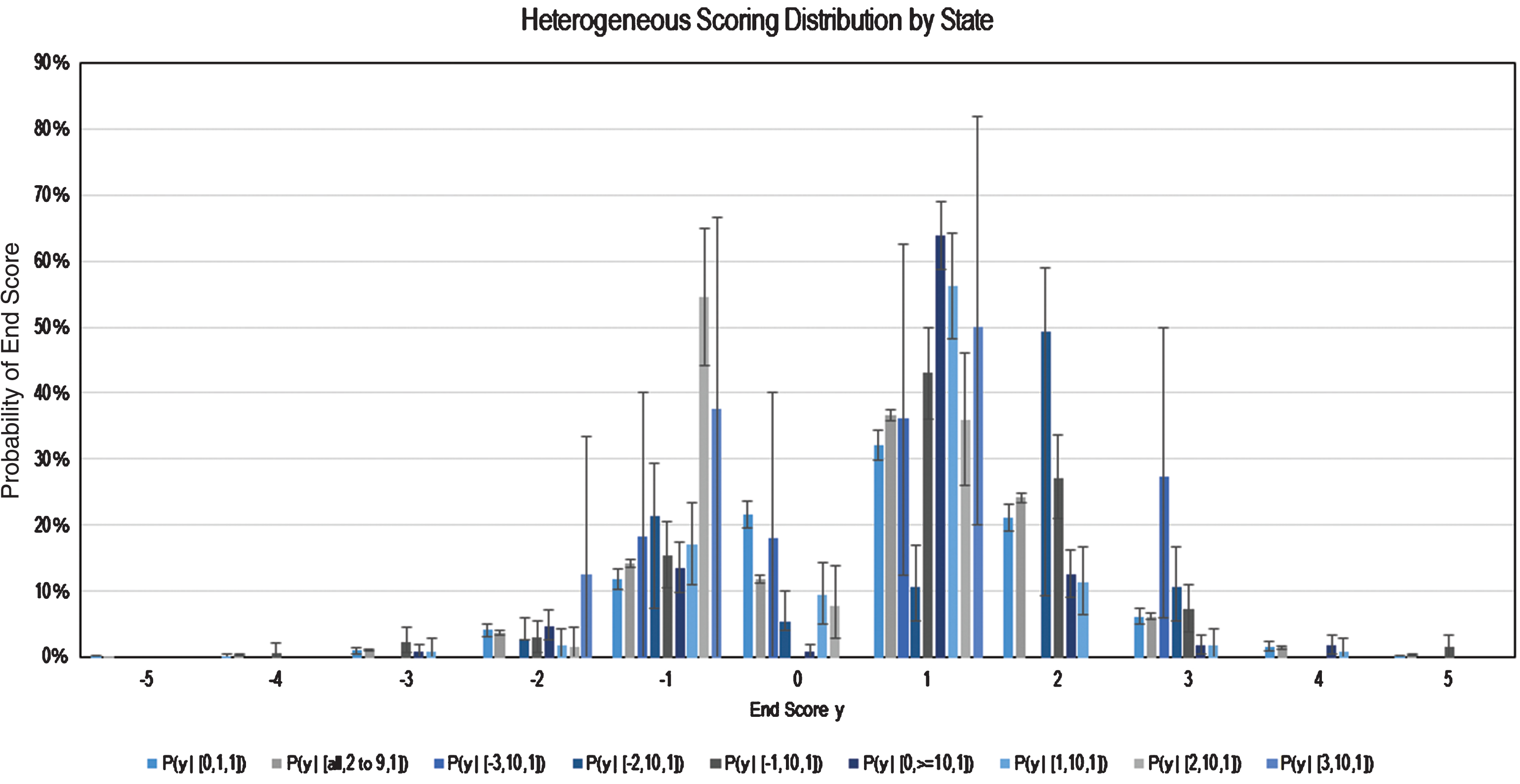
Fig.13
Alternative Visualization of Sensitivity Analysis.
Acknowledgments
The authors were students in the Yale school of Management’s Sports Analytics course taught by Professor Ed Kaplan, whom we thank for his help and guidance throughout this project.
References
1 | Ahlgren P. , (2015) , International Curling by the Numbers. World Curling Federation. |
2 | Apollo Curling. (2018) , About Curling. [online] Available at: https://www.apollocurling.com/AboutCurling.aspx [Accessed 17 Feb. 2018]. |
3 | Baumer B. , et al., (2015) , openWAR: An open source system for evaluating overall player performance in major league baseball, Journal of Quantitative Analysis in Sports, 11: (2), 69–84. |
4 | Carlson J. , (2014) , Curling has become a popular Olympic sport in U.S. [online] News OK. Available at: http://newsok.com/article/3931237 [Accessed 2 Mar. 2017]. |
5 | Cassidy P. , Cassidy , (2015) , B. Curling Canada - Championship Event Results Archive. [online] Available at: http://www.cassidys.ca/cca/brier_events.html [Accessed 4 Dec. 2015]. |
6 | Curling Canada, (2014) , Rule Changes for 2014-2018 with Rationale & Page Source. [online] Available at: http://www.curling.ca/about-the-sport-of-curling/getting-started-in-curling/rules-of-curling-for-general-play/ [Accessed 6 May 2014]. |
7 | Jarvandi A. , et al., (2013) , Modeling team compatibility factors using a semi-Markov decision process: A data-driven approach to player selection in soccer, Journal of Quantitative Analysis in Sports, 9: (4), 347–366. |
8 | Kaplan E. , et al., (2014) . A Markov model for hockey: Manpower differential and win probability added, INFOR: Informational Systems and Operational Research, 52: (2), 39–50. |
9 | Karrys G. , (2012) , Huge Curling Changes for Brier and More. [online]. The Curling News. Available at: https://thecurlingnews.com/2012/06/huge-curling-changes-for-brier-and-more/ [Accessed 6 May 2016]. |
10 | Koopmeiners J. , (2012) , A comparison of the autocorrelation and variance of NFL team strengths over time using a Bayesian state-space model, Journal of Quantitative Analysis in Sports, 8: (3). doi: . |
11 | Nadimpalli V. and Hasenbein J. , (2013) , When to challenge a call in tennis: A Markov decision process approach, Journal of Quantitative Analysis in Sports 9: (3), 229–238. |
12 | Park S. and Lee S , (2013) , Curling Analysis based on the possession of the last stone per end. Procedia Engineering, 60: ((2013) ), 391–396. |
13 | Sports Illustrated, (2012) . Sport of curling growing in popularity since Vancouver Games. [online] Available at: http://www.si.com/more-sports/2012/02/03/curling-united-states [Accessed 2 Mar. 2017]. |
14 | Wikipedia. (2015) , Curling. [online] Available at: https://en.wikipedia.org/wiki/Curling [Accessed 4 Dec. 2015]. |
15 | Willoughby K. and Kostuk K. (2004) , Preferred scenarios in the sport of curling, Interfaces, 34: (2), 117–122. |
16 | Willoughby K. and Kostuk K. , (2005) , An Analysis of a Strategic Decision in the Sport of Curling, Decision Analysis, 2: (1), 58–63. |
17 | Willoughby K. and Kostuk K. , (2006) , Curling’s Paradox. Computers & Operations Research, 33: (7), 2023–2031. |
18 | Willoughby K. , et al., (2001) , Modelling curling as a Markov Process, European Journal of Operational Research, 133: (3), 557–565. |
19 | World Curling Federation, (2015) , WCT Results API. [online]. Available at: http://resultsapi.worldcurling.org [Accessed 4 December 2015]. |
20 | World Curling Federation, (2016) , A sport united through passion. [online] Available at: http://www.worldcurling.org/history-feature [Accessed 5 May 2017]. |


