
Predicting golf scores at the shot level
Abstract
We present the only model to date that predicts the discrete probability distribution of a golfer’s score for each hole of a tournament on a shot-by-shot basis. We first generalized Broadie’s technique of score-based skill estimation to allow a golfer’s skill (e.g. scoring average, driving spray, iron play, putting) to vary continuously by time-weighting data with exponential decay. Training a single-layer 50-node neural network to predict probabilities of scoring by hole resulted in an out-of-sample cross-entropy error of 0.974. We then added features of each hole (e.g. par, green size, sand area) onto the model, representing golfers and holes in an N-by-M dimensional space and achieved an error of 0.953. Adding in course features provided by ShotLink (e.g. fairway height, firmness, wind speed) dropped error to 0.9374. Finally, generalizing the model to update probabilities per shot further reduced error to 0.891.
This work helps players understand which skill sets they should improve on, manage courses better (better to miss fairway right or left on hole 13 of Bethpage Black?) and select the best tournament to enter. It also revolutionizes the viewing experience of the PGA by live updating odds to win per shot (similar to WSOP) and helps sports books offer more accurate betting lines.
1Introduction
1.1Performance based on aggregate golfer skill factors
There have been a number of efforts to quantify a golfer’s performance. Much of the early work model performance based on aggregate golfer skill factors. These aggregate skills are means, percentages and totals representing different parts of a golfer’s game. Table 1 shows the core aggregate skill factors and the abbreviations we will use in describing previous literature.
Table 1
Aggregate Golfer Skill Factors Used in Prior Work
| Abbreviation | Name | Description |
| DRIVEDIST | Driving Distance | Average length of drive [yards] |
| DRIVEACC | Driving Accuracy | Percentage of times the drive successfully ends in the fairway [% ] |
| GIR | Greens in Regulation | Percentage of times the green is reached in regulation, which is when the number of strokes taken to reach the green (on the course) is at least two fewer than par [%] |
| SANDSAVE | Sand Save | Percentage of times the golfer gets par or better after hitting into sand trap [% ] |
| TOTALPUTT | Total Putt | Average Total number of putts made per round [puts/18 holes] |
| PUTTGIR | Putts taken on GIR | Average number of putts taken only on GIR [count] |
| PUTTNONGIR | Putts not taken on GIR | Average number of putts taken not on GIR [count] |
Davidson and Templin (1986) performed a regression over the top 119 money golfers of the 1986 PGA season to forecast scoring average and prize money earned based on driving proficiency (composed of DRIVEDIST and DRIVEACC), GIR, TOTALPUTT and SANDSAVE. They found that GIR, TOTALPUTT and driving proficiency explained 86% of a players scoring variance, with GIR being the most important skill factor [1]. Using the same dataset but considering a larger number of features that were min-max normalized, Shmanske (1992) performed a regression to model dollar winnings. His work included DRIVEDIST, DRIVEACC, GIR, SANDSAVE, TOTALPUTT, PUTTGIR and the corresponding amount of time spent in practice for each of the skills. He found that PUTTGIR, DRIVEDIST and GIR (in that order) were the three most important skills that contributed to earnings [2]. Jones (1990) also modeled money earned in 99 of the top 100 money winners of the 1980 PGA season using TOTALPUTT, DRIVEDIST and GIR. Similar to Shmanske, he found that TOTALPUTT and GIR are the two highest correlated features to earnings [3]. As an extension to the findings of Davidson and Templin, Belkin, et al. (1994) analyzed a larger dataset of PGA stats for years 1986 to 1988. Performing stepwise multiple regression (a method that doubles as a means of feature selection), they found that the most important predictors of scoring average are GIR, DRIVEACC and TOTALPUTT [4]. Dorsel and Rotunda arrived at a similar conclusion by also performing multiple regression on the same aggregate features for the top 42 players of the 1990 PGA tour [7]. They also show that GIR was the most important skill. On the contrary, Engelhardt (1995) by performing a rank order correlation between the top 10 ranked money winners and top 10 ranked in each aggregate skill category of the 1993 and 1994 PGA seasons, argued that while GIR was seen to be the largest contributor to success up to this point, the trend has now shifted to DRIVEDIST and DRIVEACC being more important than GIR [5]. Peters (2008) using the same methodology, performed his analysis with DRIVEACC, DRIVEDIST, GIR, PUTTGIR, SANDSAVE and years of experience as his regressors. His dataset comprised of tournaments in the PGA tour from 2002 to 2005. He found that PUTTGIR was the most important skill, while DRIVEDIST, SANDSAVE and years of experience were insignificant factors [6].
The studies up to this point in time made a very reasonable assumption that traditional PGA golfer aggregate skills can be used as determinants for performance. While this is generally correct, one has to question the variability of the coefficients of the regressions and the variability in which skill factors are most important across these studies. While some of this effect can be attributed to the gradual evolution of the game in time, a larger part of this discrepancy is due to the fact that these aggregate features are highly correlated, producing non-stable results. For instance, putting is correlated with GIR in that when a player hits the green in regulation, she will have a longer than average putt. In the same way, golfers who are better drivers are more primed to hit the green in regulation.
1.2Attempts at decreasing correlations between skills
Alexander and Kern (2005) realized the correlated skills problem and attempted to construct a pure measure of each skill. Using traditional aggregate stats from PGA tournaments from 1992 to 2001, they construct pure aggregate statistics for approach shots (IRON) and putting skill. They computed the former by taking the residuals when GIR was regressed from DRIVEDIST and DRIVEACC, and the latter by taking the residuals when PUTTGIR was regressed from IRON. Intuitively, this means the variation in GIR that could not be explained by DRIVEDIST and DRIVEACC can be attributed to iron playing skill, with the same being is true for PUTTGIR and putting skill. They find that pure putting skill is the most important factor that contributes to a golfer’s success (measured in earnings this time) [8]. Baugher, et al. (2014) employed the same featurization and analyzed PGA tournaments from 2006– 2013. They also show that putting skill is the most important determinant of success [9].
With the isolation of pure golfer skill factors, both authors Alexander, et al. (2005) and Baugher (2014) have also studied the change in the importance of these skills in time [8,9]. Alexander, et al. (2005) notes an increase in the marginal value of DRIVEDIST and a decrease in the value of pure putting skill in the PGA from 1992 to 2001. Among other trends, Baugher, et al. (2014) notes the increase in importance of DRIVEDIST and DRIVEACC in the PGA from 2008 to 2013. This increase in importance, as they have mentioned in their work, coincides with the decision of the PGA Tour to increase the length of the courses in time.
1.3Variability caused by course difficulty and field strength
Needless to say, changes in the course and relative golfer field strength affects performance of a golfer. Moy and Liaw (1998) compared datasets from the PGA, Senior Tour and LPGA for 1993 season and found that different leagues have different apparent skill factors for success. They report that the PGA commands a more well rounded game with PUTTGIR and GIR as the two largest factors of success, while the Senior Tour and the LPGA, due to its shorter courses, emphasize iron and putting skills [10]. Pfitzner and Rishel (2005) and Shumanske (2000) also investigate determinants of golfer success in the LPGA and how they compare to the PGA [11]. As expected, the relative importance of golfer skill factors varies across tournaments. Since golf is a ranking based sport, field strength also affects a golfer’s individual performance in terms of money earned. In later sections, we will talk more about how researchers have taken a first crack at solving this problem [11,12].
1.4Shot level analysis
In 2008, Brodie presents his work on shot level analysis, currently known as “Strokes Gained” as an alternative to the use of the traditional aggregate skill factors [14]. The idea of shot level analysis, wherein the value of a shot is measured by the difference in “state” between the location of the ball before and after the shot was first introduced by Cochran and Stobbs (1986) and Landsberger (1994), but never gained popularity due to the lack of rich data [13].
Shot level analysis provides a more granular way to evaluate performance compared to the aggregate skill factors described in early sections in that it achieves isolation of individual shots (problem discussed in section 1.b) and provides a way to distinguish large and small errors (e.g. missing the green by 1 yard or 30 yards). Equation (1) shows the base strokes gained equation for a shot.
(1)
In 2011, Brodie published an extension to his work where he computes benchmarks for average strokes to hole out not only based on distance but also based on shot type (tee, putt, recovery, etc) [15].
(2)
The tee shot function u (dist, shot _ type = tee _ shot) was modeled as a piecewise polynomial function for par-3, par-4 and par-5. Shots within 50 yard (sand, rough or fairway) were simply means over each shot type. Putting is a probabilistic model that is a combination of a one-putt and three-putt model. The one-putt model was based on an intuitive physical model developed by Holmes (1991), where a normal distribution was fit for both distance the ball will travel and the angle of putt error. The three putt model was simply selected by Brodie based on statistical data fit and is defined in equation (6) of his paper. The resulting putting model assumes four putts and above have zero probability, hence the two-putt probability is simply the probability that the golfer neither one-putts or three-putts. u (dist, shot _ type = putt _ shot) would then be the expected value of the said discrete probability distribution [15].
1.5Adjusted shot level analysis
The latter half of Brodie’s (2011) paper adjusted strokes gained based on round and course difficulty similar to the method performed by Connolly and Rendleman (2008). The golfer’s 18-hole round score was expressed as the sum of player skill (that is allowed to vary over time), course level difficulty and round level difficulty by iteratively fitting a smoothing cubic spline on time varying individual player skill and then course and then round level difficulty [16]. This allowed Brodie to rank players based on their skills in different types of shots while accounting for course and round difficulty.
2Contributions
Our contribution to the field is in the development of a model that predicts golfer scores on a shot by shot basis. This framework forecasts golf scores based on its atomic unit (a shot) similar to a pitch-level analysis of baseball data.
While prior work can be seen as predictive in nature, the goal of most past studies have been largely focused on evaluating, quantifying and comparing golfers’ performances. Our shot by shot predictions predict the discrete probability distribution of the golfer’s score in a hole based on the current state of the shot (shot number, distance from the hole, lie), golfer skill features, course features, hole features and wind speed. Predicting shot-level probabilities allows us to forecast many other quantities with simplicity. For example, one can compute hole-by-hole probabilities by evaluating the shot-probability function in the tee box state. Also, one can approximate the joint distribution of a golf tournament using Monte Carlo sampling.
The first part of our work involves the construction of individual golfer feature vector based on the golfer’s skills per shot type. As discussed above, Brodie’s assigned player skill by taking the average strokes gained per shot type of each player [15], thereby equally weighting historical skill for each shot type. Connolly and Rendlemen allow a golfer’s overall skill to vary in time [16]. We build on these by allowing each shot type skill of each individual golfer to vary in time. This involves two important considerations: normalizing data against course and round level difficulty and dynamically weighting past data to estimate current skill levels. Our method eliminates the need to arbitrarily choose a weighting schedule to assign current skill given past skill. For example, putting performance is noisier and are less repeatable than iron play. This is reflected in our data-weighting model.
The next part of our work constructs hole and course level features. As described in section 1.3., there has been previous work in quantifying holes and courses based on players’ performance on them. We introduce our method of mining spatial data to infer certain attributes of each hole.
Lastly, by the atomic nature of forecasting shot-by-shot, we are able to derive exactly how much the improvement of each individual golfer’s particular skill will contribute to his odds of winning specific tournaments, accounting not only for the course, hole and the weather, but also for the other golfers who are competing in the same tournament. This individualization is an improvement to previous studies (as presented in Section 1.1.) that are only able to compute improvements in general for an average PGA golfer. Another interesting by-product of shot-by-shot forecasting is our ability to compute live probabilities for hole scores as shots are being taken. Akin to how the world series of poker tour shows viewers probabilities to win of each player’s hand, the PGA tour can also show viewers score probabilities that can help boost viewership and engagement. This is especially practical for finding opportunities in betting markets, where a single shot can cause drastic movements to tournament-level win probabilities.
To our best knowledge, we present the most granular and comprehensive prediction model for golf.
3Dataset
We used PGA tour’s ShotLinkTM dataset [18] in our analysis. With about 250 volunteers per tournament, the dataset captures the ball location and various properties of each individual shot taken. Aside from ball coordinates and distance to hole, the dataset captures the ball’s lie, the ground slope’s, wind speed and various other features.
For our work, we consider all shots taken by all players from 2009 to 2016. There were over 8 million shots recorded within this time period. Unlike previous papers that only took the top active golfers per season, we analyze all golfers by fitting priors on golfers with less historical data. We used 2009 to 2015 as our training set and 2016 for our test set.
4Featurization
Our goal is to predict the probability distribution of a golfer’s score at any moment. This probability updates for every shot that he has taken. Before we describe the modeling, we first explore the four classes of features that we used, golfer features, hole features, course features and game-state features.
4.1Golfer features
The most important aspects to consider when constructing features that describe a golfer’s skill factors is weighing past data to measure current skill levels and normalizing observed skill based on course difficulty. The golfer skills that we ultimately want to produce are Scoring Average, Driving Distance, Driving Spray, SSG(Smoothed Strokes Gained): long approach, SSG: short game, SSG: putting (see Table 2 for more details). The terminology used in this table will be explained in later subsections.
Table 2
Golfer Features Used in the Model
| Player Feature | Description |
| Scoring Average | Adjusted scoring average |
| Driving Distance | Average Driving distance (yards) |
| Driving Spray | Mean absolute deviation of tee shots from center of fairway |
| SSG: long approach | Smoothed Strokes Gained on long approach shots |
| SSG: short game | Smoothed Strokes Gained for short approach shots |
| SSG: putting | Smoothed Strokes Gained: putting |
4.1.1Smoothed strokes gained
Broadie’s strokes gained metric has revolutionized the golf world by describing where each player gained or lost strokes over the course of a round. Some of these times, however, a golfer enjoys good luck that is not repeatable. For example, if a player makes a hole in one on a par 3 that takes the average player 3.1 shots, he receives +2.1 strokes gained to iron play. In reality, this will overestimate the player’s iron ability, as hole outs from long distances are more luck than skill. We propose an adjustment to strokes gained, called Smoothed Strokes Gained (SSG), to eliminate such noise.
The definition for SSG is simple: compute strokes gained from each shot exactly as Broadie defined it, except add on a penalty function – Stroked Drained – to shots that holed out from a long distance. We chose a Gamma CDF with shape = 3.5 and scale = 6.5 to penalize a shot that holed out from X yards. Above is a plot of strokes drained per shot made versus yards of hole out.
4.1.2Skill normalization
Normalizing a golfer’s performance based on the difficulty of the course is not a new concept and has been explored by previous authors as described in earlier sections. Equation (3) captures this method of normalization:
(3)
We basically say that for round t, the normalized quantity we assign to a player’s performance (any one of the features in Table 2) is equal to the actual observed performance vt-actual plus the difference between the average actual performance observed for all players in that round and the average pre-round skills of the same set of players. This allows us to account for players playing in different tournaments at different points in time in our model.
To compute a feature F (any of the quantities in Table (2)), we weight each player’s normalized values and regress them to the mean with a prior. For a skill F and a set of weights wt,
(4)
4.1.3Iterative updating
We iteratively update time weighted features and normalized data until the difference of the two mean terms converges. That is to say we compute the value for the feature F as stated in equation (4) and use that value as the skill we assign each player when we compute vfield-preround on equation (3). The new skills we derive are fed back to equation (4) to recompute the next iteration of weights and skills.
Table 3
Weights of different weighting methods for different skills
| Weighting Method | Scoring Average | Driving Spray | SSG: Iron Play | SSG: Putting |
| 12-week rolling average | 0.08 | 0.16 | 0.17 | 0.02 |
| Half-life 50 days | 0.17 | 0.31 | 0.18 | 0.11 |
| Half-life 150 days | 0.31 | 0.25 | 0.29 | 0.25 |
| Half-life 400 days | 0.26 | 0.14 | 0.27 | 0.21 |
| Half-life 800 days | 0.15 | 0.09 | 0.13 | 0.2 |
| Intercept | 2.16 | 0.4 | – 0.19 | 0.13 |
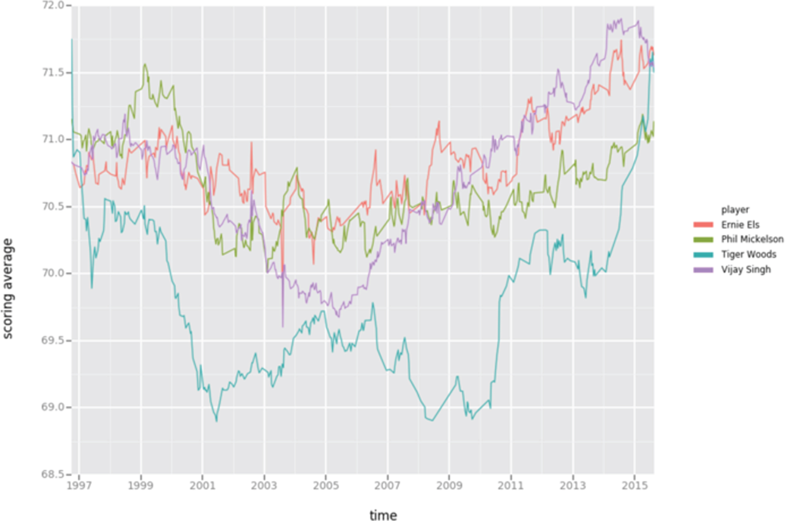
Fig.1
Featurized Scoring Average in Time for Representative Golfers.
4.1.4Weighting past data to measure current skill levels
There is a core tradeoff between sample size and recency of the data, and this tradeoff varies for different types of skills. Above, we compute each feature F by choosing a weight function wt and running the above procedure. Choosing this weight function is not straightforward; practitioners and researchers alike have made varying decisions. For example, the Sagarin rankings use a 52-week rolling average, whereas some fantasy golf players use as little as 10 rounds. We ran an ensemble over many different weighting functions wt to arrive at the best weight-of-weights for each skill.
Our goal is to predict future normalized values using some combination of past normalized values, each with a different weighting function. Coefficients with higher values correspond to stronger weighting methods. To carry this analysis out, we employed stochastic search variable selection (SSVS), a Bayesian method for model selection. The main advantage of Bayesian methods is that one can choose priors to combat the high collinearity of features. Specifically, SSVS allows one to explicitly give coefficients a high probability of equaling zero exactly. We used Zellner’s g-prior (Zellner, 1986) [17] over the coefficients and Gibbs sampling to fit the model. We present a table of coefficients for a few features in Table 3 and show a plot of one of the normalized and time weighted features, scoring average, for four representative golfers in Fig. 1.
4.2Hole features
Computing hole features was an exercise in manipulating spatial data. Hole features built include par (categorical), green size, sand area, normalized penalty strokes, and fairway width. These are shown in more detail in Table 4.
Table 4
Hole Features Used in the Model
| Hole Feature | Description |
| Par | Par of the hole, treated as a categorical variable |
| Green Size | Size of the green in square feet |
| Sand Area | Size of the sand area in square feet |
| Normalized Penalty Strokes | Average # of penalty strokes taken this hole |
| Fairway Width 250 | Width of the fairway 250 yards from the tee |
| Fairway Width 275 | Width of the fairway 275 yards from the tee |
| Fairway Width 300 | Width of the fairway 300 yards from the tee |
| Fairway Width 325 | Width of the fairway 325 yards from the tee |
| Fairway Width 350 | Width of the fairway 350 yards from the tee |
Fairway width and par values were readily available in ShotLink, while we computed the green size, sand area and normalized penalty strokes.
4.2.1Convex hull to estimate green size
Convex hull is a known technique for which given a Euclidean plane, the smallest convex set that contains all points X is computed. Figure 2 shows a visualization of convex hull.
ShotLink gives both the labeled location (i.e. Tee Box, Green) as well as the spatial (x, y, z) coordinates of each shot. To estimate the green size, we can filter for all shots from the Green and compute the convex hull around these points to estimate the size. On average each green has about 700 putts on it per standard tournament, giving us enough data points for a decent estimate. Figure 3 shows an example of hole 1 at Silverado CC in Napa, California.
Fig.2
Convex Hull of a set of points.
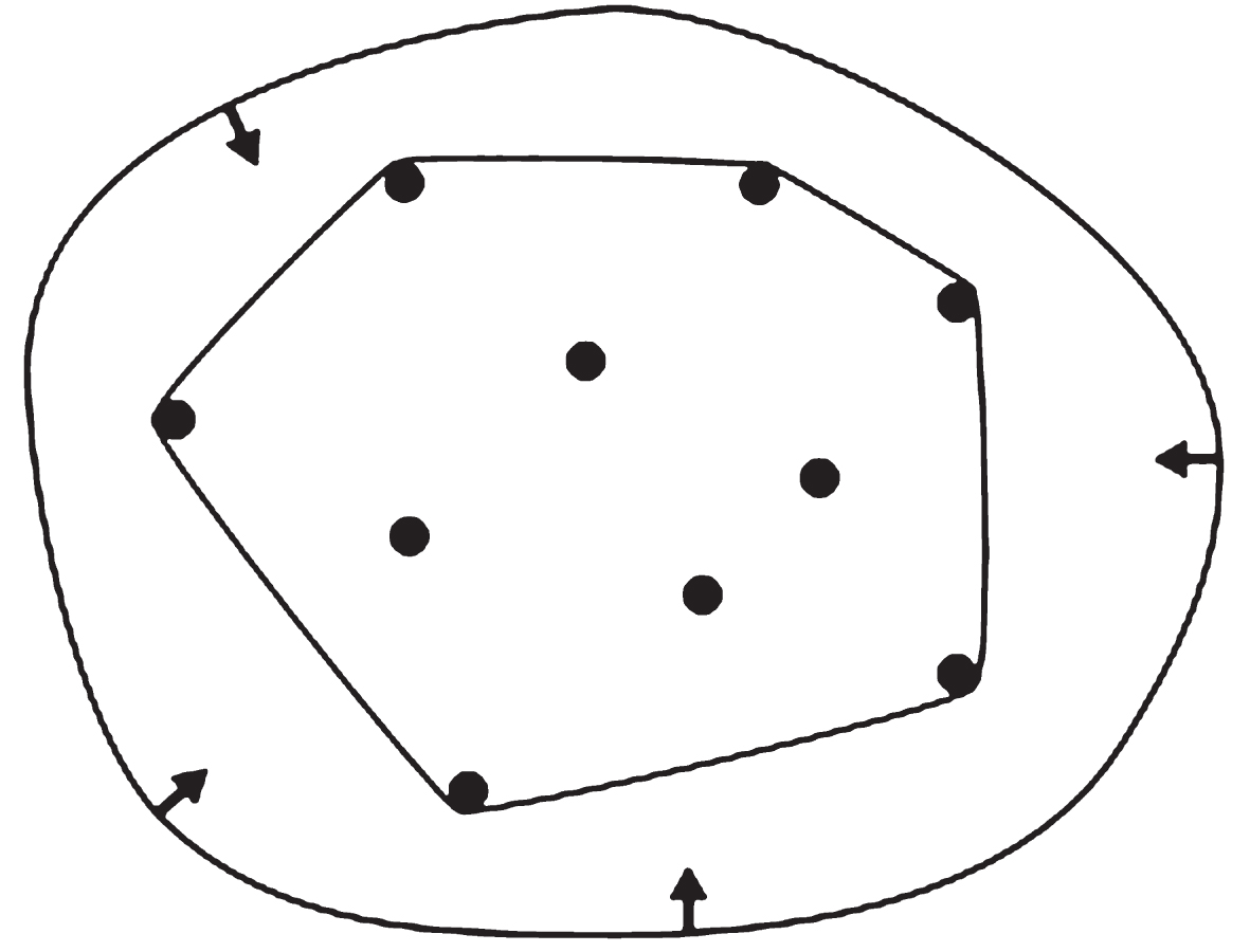
Fig.3
Putts on the Green of Hole 1 in the Safeway Open.
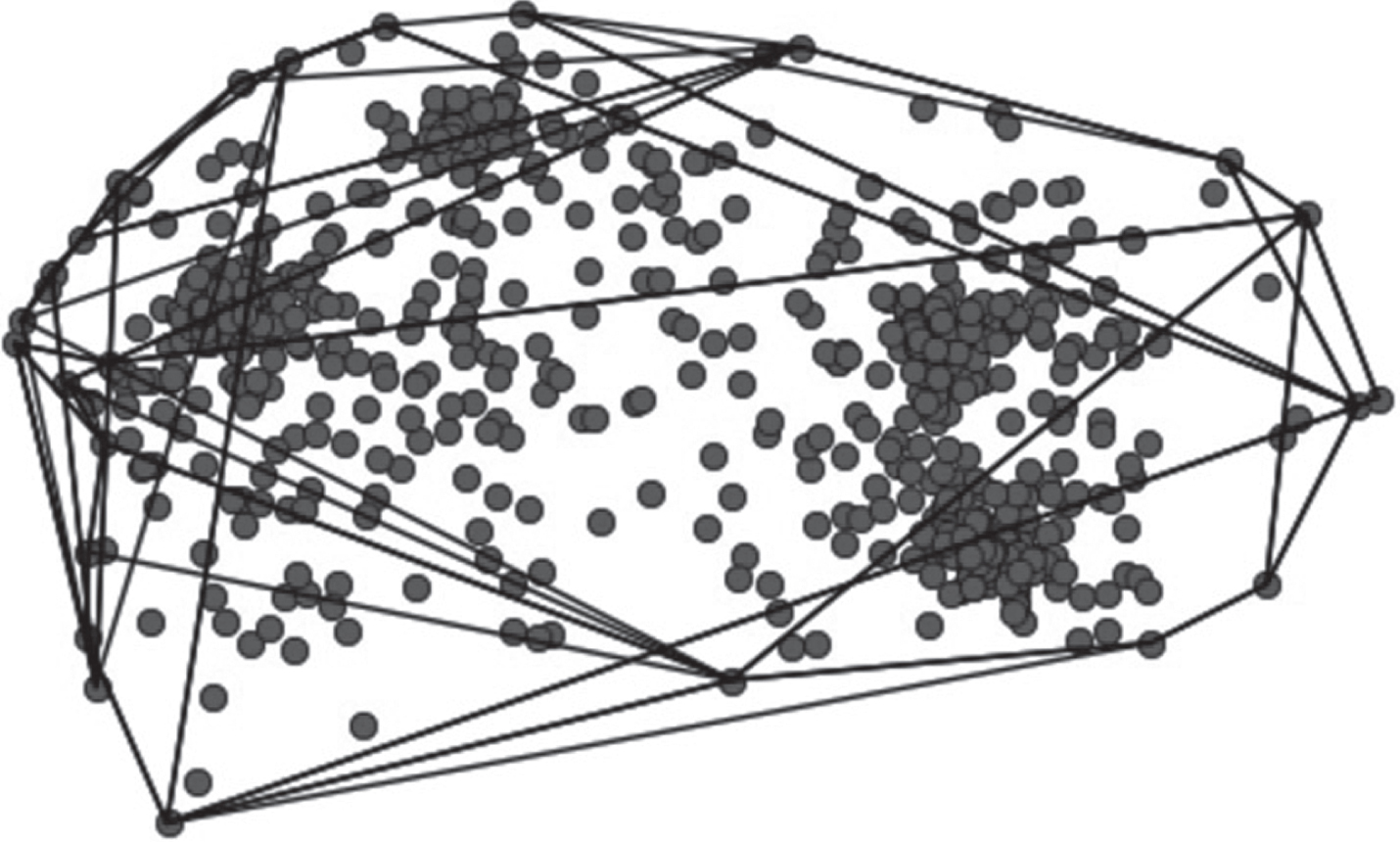
The reason convex hull is ideal for putts on the green is because there is only one green per hole. This is not the case for sand bunkers, hence we employ K-nearest neighbors to classify points in the space. It is no coincidence that the points above form four clusters. Each cluster corresponds to a round of the tournament; the course superintendent changes the location of the hole after each round. Note that this method will slightly underestimate the size of each green, as there will be locations on the green outside the hull boundary on which no shots are recorded.
4.2.2K-Nearest neighbors to estimate the size of sand bunkers
Using the (x, y, z) coordinates labeled as sand bunkers in ShotLink, we employ K-nearest neighbors with K = 1 to classify all points in the course. While data scientists rarely choose K = 1, this context is an exception: once we know the label of an (x, y, z) coordinate, it will not change. In addition, increasing K will bias toward predicting the most common locations (the fairway or the green).
4.3Course features
Computing for course features was more straightforward as most features came directly from ShotLink and only needed minor validation. Course features that we computed are shown in Table 5. They include difficulty, fairway height, rough height, stimp, wind speed, fairway firmness and green firmness. The only feature that we derived was the difficulty feature for the course. This was computed by taking the residual of when actual scoring average is regressed with the scoring average feature; that is, the difference of mean terms from 4.1.2.
Table 5
Course Features Used in the Model
| Course Feature | Description |
| Difficulty | Difference between field’s scoring skill and observed scoring average |
| Fairway Height | Height of the fairway in inches |
| Rough Height | Height of the rough in inches |
| Stimp | Stimpmeter rating of the green |
| Wind Speed | In miles per hour |
| Fairway firmness | As rated on a scale from 1 to 3 |
| Green Firmness | As rated on a scale from 1 to 3 |
4.4State features
The last set of features used were game state features. These features are purely descriptive in nature, and just spell out the state of the ball when predictions are made. The two features that describe state are distance from hole and lie. Table 6 explains these features.
Table 6
State Features Used in the Model
| Hole Feature | Description |
| Distance From Hole | Distance in yards from the hole |
| Lie | Categorical variable describing the current lie of the shot (e.g. green, sand bunker, fairway, etc) |
5Summary results
We trained on ShotLink PGA 2009 – 2015 data and held out 2016 as a test set. We excluded putts from less than 4 feet when evaluating, as putts from inside this range are holed with a very high probability regardless of the player, hole or setting.
To establish a benchmark, we trained a single hidden layer neural net of 50 nodes with golfer skill features described in section 4.1 and hole par. This resulted in an out-of-sample cross (OOS) entropy error of 0.974. Examining the results, we clearly saw that scoring errors were mainly due to longer and shorter holes with the same par. We added in hole length and an interaction feature between hole length and driving distance skill and retrained the model to achieve an OOS error of 0.953.
We trained a more comprehensive neural net with all the features described in section 4, golfer skill features (section 4.1), hole features (section 4.2), course features (section 4.3) and game state features (section 4.4). The full model resulted in an OOS error of 0.937.
Lastly, we re-featurized our dataset to predict scores on a shot-by-shot basis. This was a simple transformation where we updated the distance to the hole based on the (X, Y) coordinates of the ball provided by ShotLink and updated the prediction result by subtracting the number of shots taken for the hole thus far from the final hole score.
We used three algorithms to forecast shot-by-shot probabilities: softmax regression, random forests and a single-layer neural network. For the regression, we allowed the following interactions: driving spray and fairway widths, driving accuracy and rough height, SSG: approach and bunker area and SSG: long approach and green area. We allowed 50 estimators in the Random Forest and maintained the same single hidden layer neural network of 50 nodes. Softmax regression resulted in an OOS cross-entropy error of 0.924, random forest resulted in an OOS cross-entropy error of 0.903 and neural net results in an OOS cross-entropy error of 0.891. These results are summarized in Table 7.
Table 7
Model Results
| Model | OOS Cross Entropy Error |
| (Benchmark) Skill + par only Neural Network | 0.974 |
| (Benchmark) Add in hole length to Neural Network | 0.953 |
| Hole level: All features Neural Network | 0.937 |
| Shot level: All features Softmax Regression | 0.924 |
| Shot level: All features Random Forest | 0.903 |
| Shot level: All features Neural Network | 0.891 |
Here are some examples of the model’s predictions. In the 2016 Players Championship, on Jason Day’s R3, 15th hole 4th shot, the ball starts a few feet just outside the green. At that point the model predicted Jason’s score probabilities for the hole to be < par: 0.15, bogey: 0.81, double bogey: 0.03, double bogey+: 0.01 > . Jason ends up saving the par and proceeds to win the tournament decisively. In the 2016 U.S. Open, on Dustin Johnson’s R4, 18th hole 2nd shot, his probabilities were < eagle: 0.012, birdie: 0.09, par: 0.73, bogey: 0.16, double bogey: 0.01, double bogey+: 0.009 > . Dustin makes the birdie and wins the U.S. Open.
6Conclusions
We presented a granular forecasting model for the PGA by leveraging its ShotLink dataset. The result is a function that computes a probability distribution over each possible score on a hole, given a player’s state and skill level, difficulty of the hole and course conditions. Furthermore, these state variables are accessible in real-time, which motivates exciting applications. Applications that range from player development, course management, and tournament selection to audience engagement and improved sports books can easily be derived from this model.
References
1 | Alexander D.L. and Kern W. (2005) . Drive for Show and Putt for Dough?: An Analysis of the Earnings of PGA Tour Golfers, Journal of Sports Economics 6: (1), 46–60. |
2 | Belkin D.S. , Gansneder B. , Pickens M. , Rotella R.J. and Striegel D. , (1994) . Predictability and Stability of Professional Golf Association Tour Statistics, Perceptual and Motor Skills 78: , 1275–1280. |
3 | Baugher C. , Day J. and Burford E. , (2014) . Drive for Show and Putt for Dough? Not Anymore, Journal of Sports Economics 17: (2), 207–215. |
4 | Brodie M. , (2008) . Assessing Golfer Performance Using Golf Metrics, Science and Golf V: Proceedings of the 2008 World Scientific Congress of Golf 253–262. |
5 | Brodie M. , (2012) . Assessing Golfer Performance on the PGA Tour, Interfaces 42: (2), 146–165. |
6 | Connolly R. and Rendleman R. , (2008) . Skill, Luck and Streaky Play on the PGA Tour, Journal of the American Statistical Association 103: (481), 74–88. |
7 | Davidson J.D. and Templin T.J. , (1986) . Determinants of Success Among Professional Golfers, Research Quarterly for Exercise and Sport 57: (1), 60–67. |
8 | Dorsel T.N. and Rotunda R.J. , (2001) . Low Scores, Top 10 Finishes, and Big Money: An Analysis of Professional Golf Association Tour Statistics and How These Relate to Overall Performance, Perceptual and Motor Skills 92: , 575–585. |
9 | Engelhardt G.M. , (1995) . It’s Not How You Drive, It’s How You Arrive’: The Myth, Perceptual and Motor Skills 80: , 1135–1138. |
10 | Jones R. , (1990) . A correlation analysis of the Professional Golf Association (USA) statistical rankings for 1998, In Cochran A. (Ed.), Science and golf: Proceedings of the first World Scientific Congress of Golf. London: Spon, pp. 165–167. |
11 | Landsberger L. , (1994) . A unified golf stroke value scale for quantitative stroke-by-stroke assessment, Proceedings of the World Scientific Congress of Golf pp. 216–221. |
12 | Moy R.L. and Liaw T. , (1998) . Determinants of Professional Golf Tournament Earnings, The American Economist 42: , 65–70. |
13 | Peters A. , (2008) . Determinants of Performance on the PGA Tour, Issues in Political Economy, 17: . |
14 | Pfitzner C.B. and Rishel T. , (2005) . Performance and Compensation on the LPGA Tour: A Statistical Analysis, International Journal of Performance Analysis in Sport, University of Wales Institute, Cardiff 5: (3). |
15 | Shmanske S. , (1992) . Human Capital Formation in Professional Sports: Evidence from the PGA Tour, Atlantic Economic Journal 20: (3), 66–80. |
16 | Shmanske S. , (2000) . Gender, Skill and Earnings in Professional Golf, Journal of Sports Economics 1: (4), 385–400. |
17 | ShotLink, (2017) . PGA Tour, Available at: http://www.shotlink.com/. |
18 | Zellner A. , (1986) . On Assessing Prior Distributions and Bayesian Regression Analysis with g-prior Distributions, Bayesian Inference and Decision Techniques: Essays in Honor of Bruno De Finetti 6: , 233–243. |


