
A Bayesian perspective of middle-batting position in ODI cricket
Abstract
The cricket fraternity described “an unsettled batting position of number four” as one of the major causes for India’s exit from International Cricket Council Men’s World Cup 2019. Consistent chopping and changing batsmen at the sensitive fourth batting position proved to be a disaster for team India then. Therefore, ranking of all the batsmen, in the then Indian cricket team, who were deemed to be eligible for this position remained a much-debated issue both before and after the World Cup 2019. In the present paper, Kaplan-Meir curves are used to make multiple comparisons for respective batting performances among the batsmen who have ever played in the middle order position. In this paper, frailty of these batsmen is studied through Bayesian analysis at the start of their innings and during the time-interval of transition to their best playing ability by considering respective run scores. Posterior summaries of innate player ability are obtained by deploying a Markov Chain Monte Carlo algorithm which is then used to assess and compare the individual batting performances. Estimation of incomplete innings is handled via censoring strategies.
1Introduction
Game of cricket is played in three distinct formats: Test Cricket, One Day International (ODI) and Twenty20 (T20). One-day cricket was introduced in the 1960s as an alternative to the Test Cricket characterized by more aggressive batting, colorful uniforms and fewer matches ending in draws. ODI cricket is limited to fifty overs. The biggest event in ODI cricket takes place after every four years when the World Cup of Cricket (WCC) is organized by the International Cricket Council (ICC) which is the global governing body for cricket games. Later in 2003, T20 form of the cricket game was introduced with focus on gaining wider audience and with + emphasis on power hitting. Cricket in T20 format is limited to twenty overs. The present research is related to the game of ODI. Swartz et al., 2009 describe the play structure and related terminologies in detail.
Batting is the heart of cricket and bowling is its backbone. Cricket knowledge tells us that batting is more difficult early in a player ‘s innings but becomes easier as players familiarize themselves with the pitch conditions. A player’s batting ability is primarily assessed based on their batting average. However, in a cricket match a player never begins an innings while batting to the best of his ability as it takes time to adjust both physically and mentally to the specific match conditions. This process is nicknamed as getting eye-in which is shaped by factors such as the pitch conditions and opposition strategies. According to cricket experts a batsman is supposed to get his eye-in after he looks very comfortable in hitting boundaries (sixes and fours) and this confidence comes to a batsman after spending some time on the crease which enables him to read the pitch conditions and the bowler’s strategy against him. In other words, a batsman is said to be ‘set’ when he gets his eye-in. Batsmen are regularly seen to be dismissed early in their innings while still familiarizing themselves with the field conditions, which suggests that the probability of a batsman being dismissed on their current score (called the hazard) remains high regardless of their current score. Quantifying how well a batsman is expected to perform at a given stage of his innings identifies his batting potential could assist in the team selection strategy.
India lost the semi-final game of ICC ODI world cup 2019 (WC19) against New Zealand. Team India (TI) was super favourite and was expected to be champion for the third time in ODI world cup cricket history. Despite good play, excellent form of each player and presence of a dynamic opener (Rohit Sharma), an aggressive captain (Virat Kohli), the calm strategist (MS Dhoni), along with the other exceptionally talented players TI could not enter the final game.
There may have been a variety of reasons for India’s defeat but according to the great cricket experts like Sunil Gavaskar, Sachin Tendulkar and other seasoned cricketers it was the unsuitable player-selection at the crucial ‘number four batting position’ (N4), since almost two years prior to the WC19. According to the experts, consistent chopping and changing of TI players in the playing eleven and failure to fix mid-batting order led to loss in self-confidence of the batsman and hence his ability to play with a clear mind set, which is known to hamper the best playing ability (BPA) of a cricketer. N4 is a huge responsibility for any batsman in ODI cricket because he is expected to instantaneously pick up the pace of the innings with which the top order batsmen are batting or have batted. In other words, batsman at N4 needs to assess the batting conditions very quickly and take the ‘least time’ to get his eye-in which represents the transitional time interval between the initial playing ability and BPA. The uncertainty and instability for N4 started after the great number four Yuvraj Singh left the Indian ODI squad twice, first due to his health condition after ODI ICC world cup 2011 and then again in June 2017.
Though WC19 preparation started a couple of years ago yet TI remained indecisive regarding player at the crucial N4. From August 2017 to July 2019, India tried and tested seven batsmen, namely Ajinkya Rahane, Ambati Raydu, KL Rahul, Dinesh Kartik, Rishabh Pant, Vijay Shankar and Kedar Jadhav, who had played a minimum of two innings at N4. Rishabh Pant and Vijay Shankar were finally positioned for mid-batting order in the WC19. MS Dhoni, Manish Pandey and Hardik Pandya have also played at N4 on some occasions but they were never considered as front runners for N4 by the TI’s management committee. Post WC19, Shreyas Iyer has consistently played at N4.
The present paper focuses on the analysis and comparison of the batting performances of all the eight TI players who have played at number four position in ODIs after July 2017 till December 2020, initially through survival probabilities which are estimated, for the first time in this paper, through Kaplan Meir method and subsequently through Bayesian formulation adapted from Stevenson and Brewer (2017). The present paper is motivated by the idea of ‘initial’ and ‘eye in’ states to decide about the choice of the middle order batsmen. Concept of ‘positional cohort’ with respect to N4 batsmen is explored through Bayesian discrete event modelling in the present paper. Bayes methodology takes care of the so called ‘curse of dimensionality’ and use of statistical models easily handles the challenges which are posed by the unpredictable and inconsistent nature of the game of cricket. Analytical study of N4 assessment is important for any cricket team to select a robust line-up of batsmen.
Objective of the present work is to predict the batting abilities for the mid-order batsmen. The paper is organized in six sections. Literature review related to the statistical studies on cricket performances is presented in Section 2. Section 3 describes the N4 backdrop for the data selection. Analysis strategy and the proposed model are outlined under Section 4. Section 5 undertakes empirical survival analysis of the batsmen at N4. Section 6 is devoted to the posterior analysis of the data. Section 7 concludes the study.
2Existing parametric and non-parametric methods
Data rich nature of cricket has been utilized by numerous studies to optimize player and team performance. See for instance Clarke, 1988; Clarke & Norman, 1999; Preston & Thomas, 2000. Clarke & Norman, 2003; Swartz et al., 2009; Norman & Clarke, 2010 focus on the decision making in cricket. Davis et al. (2015) explore a novel metric for the notion of ‘expected run differential’. Jayalath, 2018 focuses on the identification of significant predictors of ODI games, which have potential to influence the outcome of a game. Goel et al., 2021 study match prediction under dynamic updation as the game of cricket progresses.
Elderton & Wood, 1945 support the claim that a batsman’s score could be modeled using a geometric progression. Kimber & Hansford, 1993 state that geometric assumption does not necessarily hold for all players, due to its difficulty in fitting the inflated number of scores of 0 appearing in many players’ career records. Bracewell & Ruggiero, 2009 proposed to model the players’ batting scores based on the ‘Ducks ‘n’ runs’ distribution, using a beta distribution to model scores of zero, and a geometric distribution to describe the distribution of non-zero scores.
An advantage of estimating hazard function is that it allows us to observe how a player’s dismissal probability (and hence their batting ability) varies over the course of their innings. While Kimber & Hansford, 1993 found batsman were more likely to get out early in their innings, due to the sparsity of data at higher scores these estimates quickly become unreliable and the corresponding estimated hazard function is observed to jump erratically between the scores. Cai et al., 2002 address this issue by using parametric smoother on the hazard function. However, given the underlying function is still a non-parametric estimator the problem of data sparsity remains an issue and continues to distort the hazard function at higher scores. Damodaran, 2006 provided a method which allows for within-innings comparisons, but lacks a natural cricketing interpretation. On the other hand, Koulis et al., 2014 proposed a Bayesian stochastic model for evaluating performance based on the player’s form, however his focus remained only on inter-innings comparison in terms of batting ability, rather than intra-innings comparison.
Swartz et al., 2009 proposed simulator for simulation of one-day cricket matches, where the outcome probabilities are estimated from historical data which produce realistic results, with a caution for continuously updating the database. Brewer, 2008 proposed an alternative Bayesian parametric model to estimate a player’s current batting ability (via the hazard function), given his score, using single change-point model. This allows for smooth transition in the hazard between the batsman’s ‘initial’ and ‘eye in’ states, rather than the sudden jumps of Kimber & Hansford, 1993 and of Cai et al., 2002. Thus, one assumes that batsmen are more susceptible early in their innings and tend to perform better as they score more runs.
3Data
Survival times of players who get out during the match are completely known. However, survival times of the batsmen who remain at crease by the end of match are said to be censored. One can refer to Lee and Wang, 2003 for statistical definitions and concepts related to survival times and survival distribution. ODI innings of all the players who were declared as front runners for N4 either by the TI management or by the selectors at different points of time are accessed (Table 1). Ajinkya Rahane had emerged as the best choice for N4 during TI’s tour to South Africa in January 2018, owing to the seaming conditions at the pitch. He then played five innings in the six match ODI series. In July 2018, KL Rahul had played two innings at N4 against England. In the same series, Dinesh Kartik was brought up at N4 to play a single inning against England and thereafter he continued to play at N4 in Asia Cup, Dubai during September 2018. After Asia Cup, Ambati Raydu assumed N4 until the start of WC19. An interestingly surprise call was made by TI’s chief selector for N4 to be assigned to Vijay Shankar. However, due to an injury incurred by him, just after playing two games in WC19, Rishabh Pant was declared N4 batsman for WC19.
argethispage2pt
Table 1
Batting scores of TI players in ODIs at N4 from August 2017 to December 2020
| Player | Score (* indicates the not-out scores) |
| Ajinkya Rahane | 79, 11, 8, 8,34* |
| Ambati Raydu | 22*, 73, 22, 100, 0, 24, 13*, 47, 40*, 0, 90, 13, 18, 2 |
| KL Rahul | 0, 9, 17, 6, 108, 26 |
| Shreyas Iyer | 7, 44*, 103, 52, 62, 2, 38, 19, 70, 53, 7 |
| Dinesh Kartik | 64*, 0, 26*, 21, 33, 31*, 37 |
| Rishabh Pant | 26, 32, 48, 4, 32, 20, 0 |
| Vijay Shankar | 29, 14 |
| Kedar Jadhav | 1, 5*, 12 |
Source: http://www.google.com.
4Methodology
Table 1 presents the scores at which the batsmen got out and their not-out scores in ODIs played by them during July 2017-December 2020. Latter are marked with * in the table. In this paper not-out scores are considered as the right censored survival data and the remaining scores as complete survival data.
4.1Kaplan meir estimates
We adopt a non-parametric approach for generating survival function for individual players. Survival probabilities are generated using product-limit method developed by Kaplan & Meier, 1958. The survival probability estimates are graphed as survival distribution known as Kaplan-Meir (KM) curves. KM curves are used for comparing batsmen’s performance. KM curves (Figs. 1–5) represent survival probability over the study period for all players under study. In the present paper, survival events represent total runs scored by an individual player before getting out in an innings. The career period, considered for the present analysis, is regarded as the survival time. The ODI in which a player does not get out is regarded as a right censored survival time. For making a fair comparison we have considered pairs of players with equivalent number of innings. For example, Shreyas Iyer having played 11 innings is compared with Ambati Raydu’s last 11 innings out of his total 14 innings played at N4 before WC19. Similarly, survival probabilities through KM estimates are compared for Dinesh Kartik, Rishabh Pant and KL Rahul taking a pair of two with their latest survival times or batting scores at N4. Thus, five pairs of players are assessed through KM analysis.
Fig. 1
KM curves for batting scores of Shreyas Iyer and Ambati Raydu.
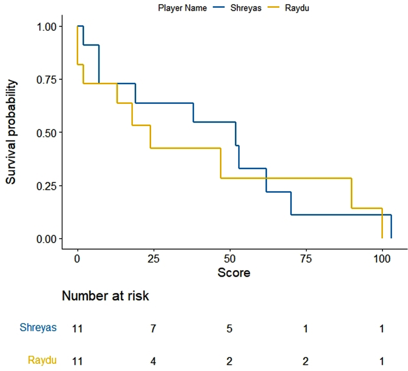
Fig. 2
KM curves for batting scores of Dinesh Kartik and KL Rahu.
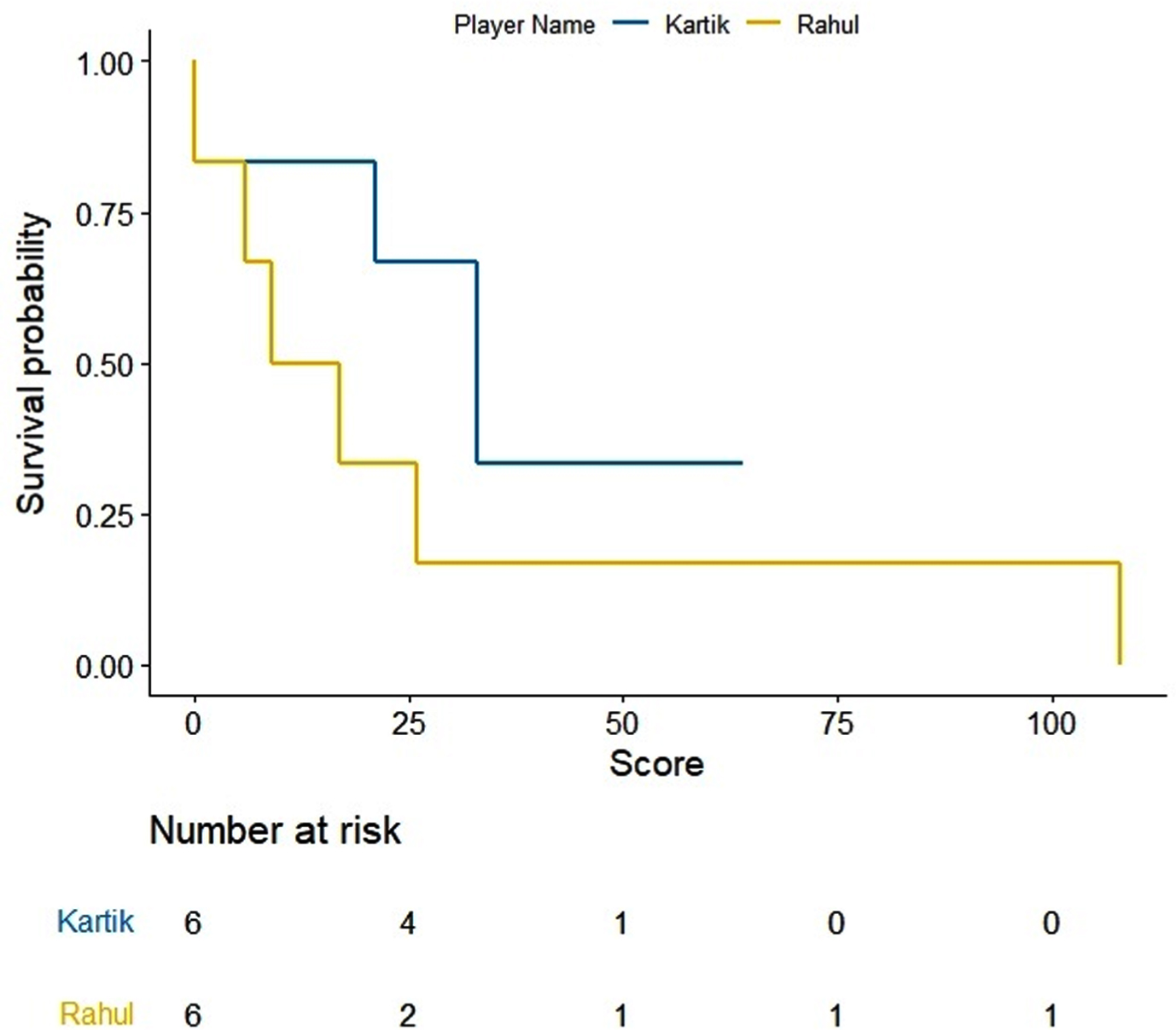
Fig. 3
KM curves for batting scores of KL Rahul and Rishabh Pant.
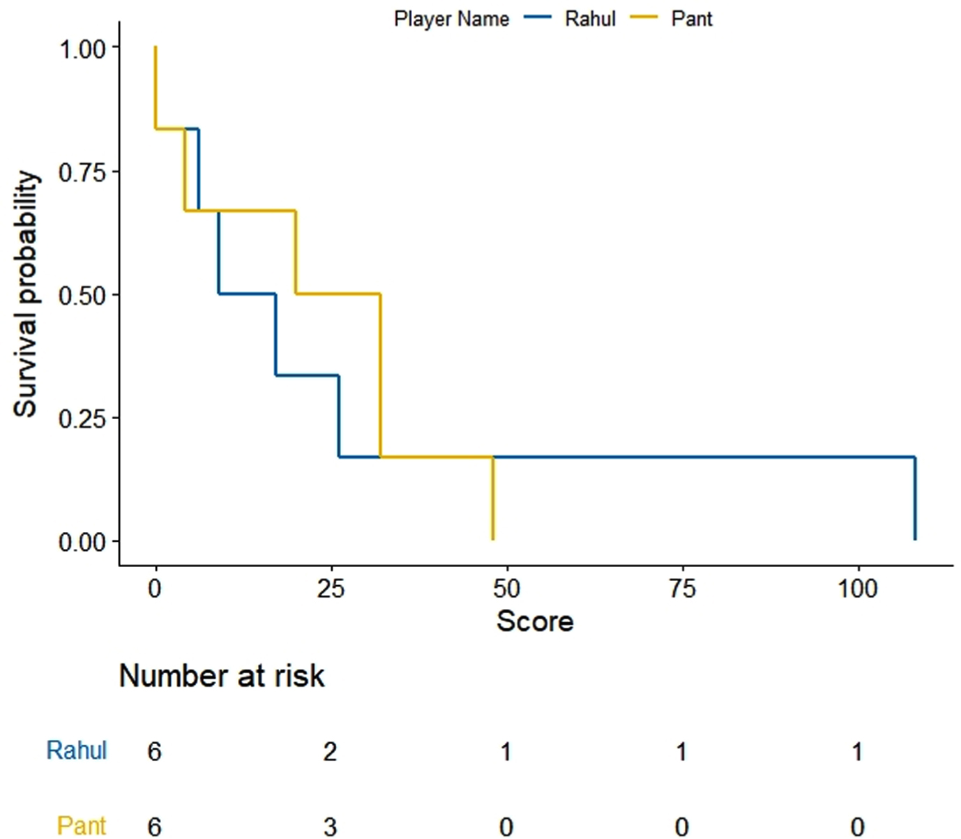
Fig. 4
KM curves for batting scores of Dinesh Kartik and Rishabh Pant.
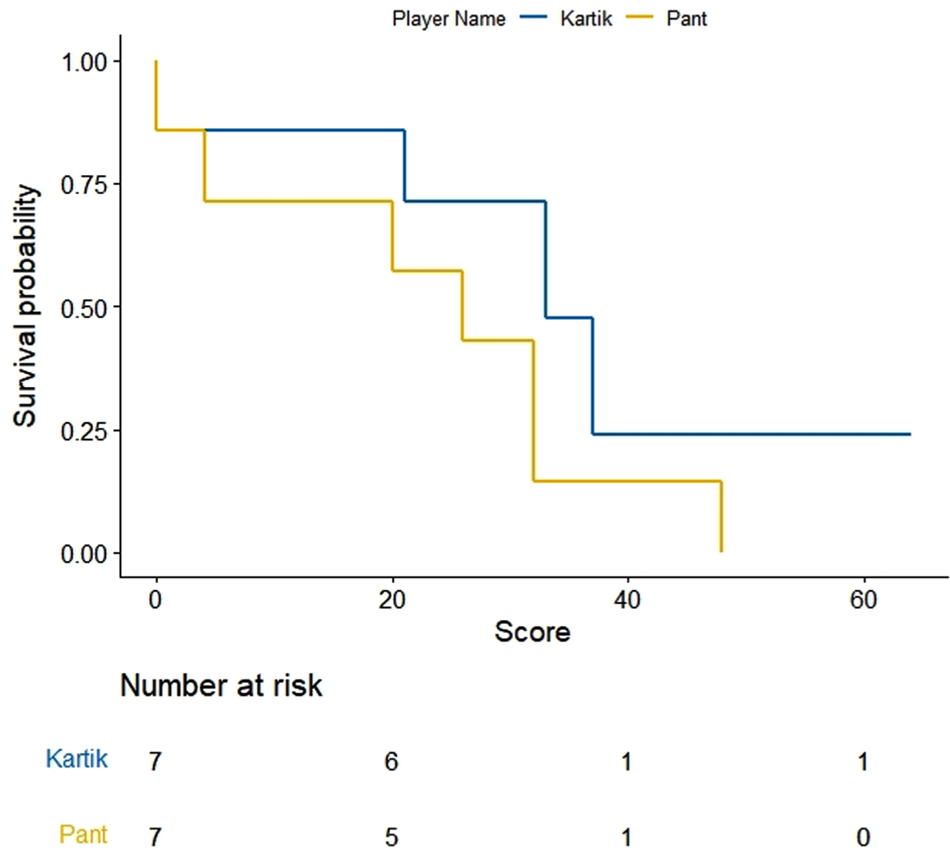
Fig. 5
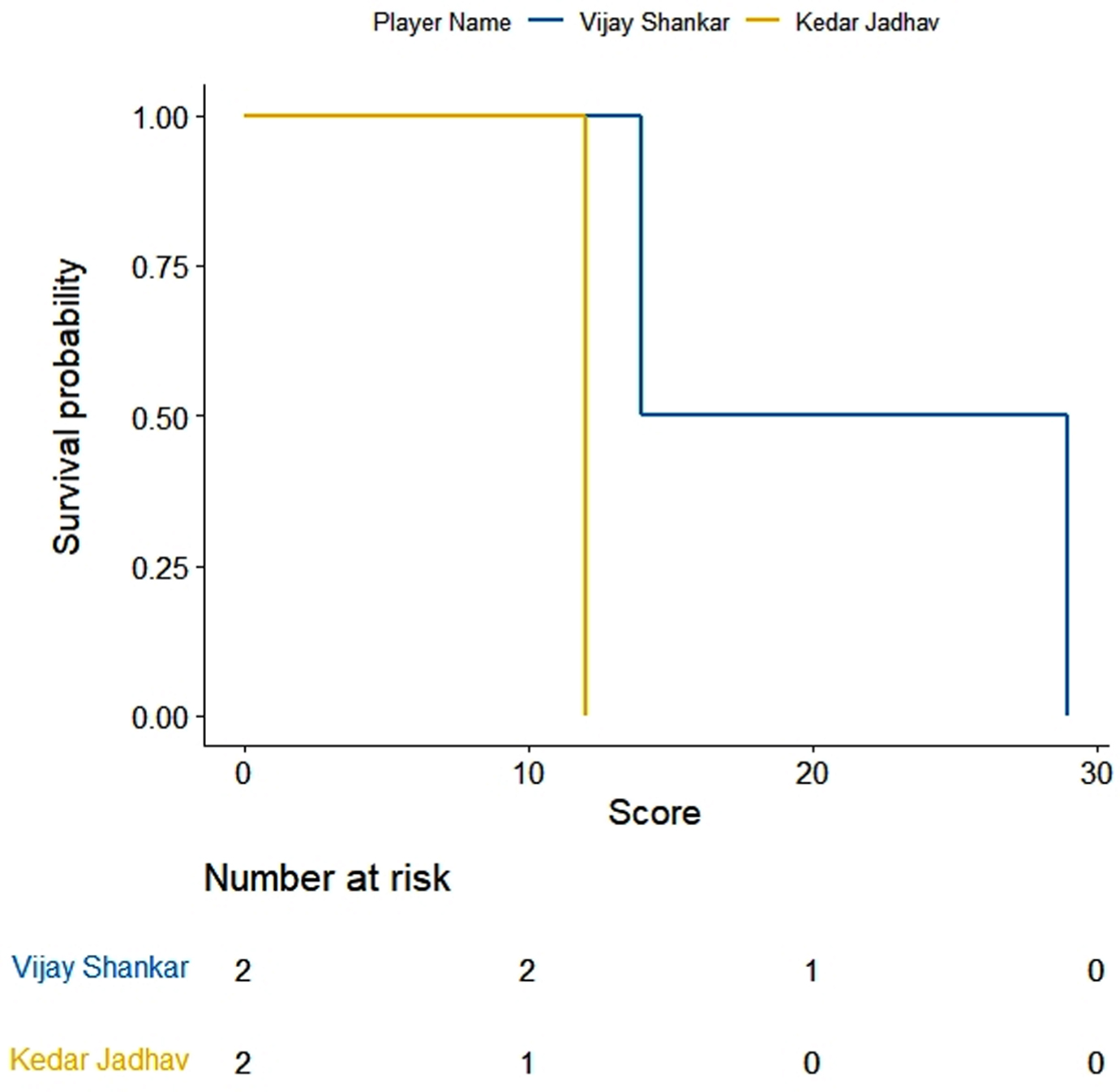
KM curves for batting scores of Vijay Shankar and Kedar Jadhav.
4.2Bayesian model
Bayesian methods are primarily preferred as they overcome the small number problem (Gelman and Price, 1999) in field data. Bayesian principle appears as a mechanism which efficiently implements the likelihood principle (Robert, 2001). Bayes approach takes care of the nuisance parameter in the likelihood function (Basu,1988). Bayes principle also facilitates incorporation of information beyond recorded data through prior distributions. Other advantages of using Bayesian approach for such analysis include its capability to account for missing data, measurement error, incompatible data, and ecological bias (Haining & Law, 2011). Posterior summaries thus obtained have been found to be robust and more precise than those obtained from the classical inference (Zellner, 1995).
Following the notations of Stevenson and Brewer, 2017, the effective batting average, mi is expressed as,
(1)
μ1, the initial batting average is defined as the average with which batsman arrives at the crease. μ2 the final batting average or the eye-in batting average which characterises the BPA of a batsman. The transition time (L) between the initial and BPA is the number of runs required to make this transition and is also termed as e-folding time. Stevenson and Brewer, 2017 place analogy between the e-folding time and ‘half-life’ thereby signifying the number of runs to be scored for 63% of the transition between μ1 and μ2 to take place.
Model (1) provides a basis for comparison among all the N4 players in the terms of BPA i.e., their ‘eye-in’ batting average and the number of runs scored to make the transition between their initial ability and BPA.
Model assumptions:
(1) Xi represents the score of a batsman in the ith innings and is assumed to follow Poisson distribution with mean mi.
(2) The batsman’s ability will not decrease after arriving at the crease, hence μ1≤μ2.
(3) Transition between the two batting states cannot be any larger than the player’s ‘eye in’ effective batting average, therefore, the value of L≤μ2.
In order to incorporate the above assumptions as constraints, we parameterize from (μ1, μ2, L) to (C, μ2,D) such that μ1 = Cμ2 and L = D μ2, where C and D are restricted to the interval [0, 1]. The effective average model is now translated as,
(2)
(3)
Since final batting average depends on the final score at which the player gets out, hence the score Xi will include scores for those innings in which batsman had got out. Not-out scores have therefore been excluded from further analysis. In the present paper, the criteria for comparison are that the batsman with higher eye-in average is considered as better and if eye-in averages are nearly same for two batsmen then comparison will be made in terms of parameter L i.e., the number runs required to make the transition between initial and best playing ability. The player with lesser L value will be regarded as a finer player.
Under Bayesian paradigm one can report parameter estimates in terms of posterior probabilities. Based on the collective batting performances in ODI matches, in the present paper a threshold of 40 runs for μ2 and threshold of 20 runs for parameter L is set up. There can be different choices for threshold of μ2 and L, but keeping in mind dynamics of ODI, a batsman getting out at 40 runs and is not taking more than 20 runs to transit from its initial playing to best playing ability is considerably good for team’s point of view. Authors calculate posterior probability for a batsman’s best playing average (μ2) to be greater than 40 runs and probability for e-folding(L) time to be less than 20 runs (Table 2). This calculated posterior probability for each batsman enables comparison for batting performances with stronger evidence. Specifically, for Ambati Raydu and Shreyas Iyer whose μ2 remains close to each other (Table 2).
Table 2
Posterior estimates and posterior probability for players whose batting capabilities were assessed through Bayesian model
| Player | μ1 | μ2 | L | 95% C.I. (μ2) | 95% C.I. (L) | P (μ2 > 40) | P (L < 20) |
| Ajinkya Rahane | 2.176 | 21.3 | 11.8 | (16.86,26.02) | (6.01,17.54) | 0 | 0.9728 |
| Ambati Raydu | 0.3519 | 43.8 | 22.35 | (39.37,48.97) | (16.96,28.47) | 0.9397 | 0.2018 |
| Shreyas Iyer | 1.753 | 42.97 | 14.67 | (38.77,47.46) | (10.59,19.7) | 0.9753 | 0.8843 |
| Rishabh Pant | 0.7142 | 19.97 | 7.351 | (16.72,23.52) | (3.515,11.77) | 0 | 1 |
| KL Rahul | 0.6896 | 29.2 | 16.5 | (24.44,34.46) | (10.54,22.95) | 0 | 0.8611 |
| Dinesh Kartik | 1.002 | 16.98 | 2.55 | (13.86, 20.55) | (0.06789, 7.356) | 0 | 1 |
4.2.1Prior specifications
Experts believe that a batsman in an ODI match gains a lot of confidence after hitting his first boundary and that is the time when he starts gaining his confidence to play his shots. This subjective opinion is incorporated as prior density in the model. Priors on the parameters of the proposed model are chosen so as to reflect this common cricket knowledge. Batting average cannot be negative and Gamma distribution has a non-negative support. The prior elicitation for the parameter μ2 is, therefore, taken as Gamma (12, 3) where mean eye-in batting average of four runs is assumed. Mean initial batting abilities and e-folding times are regarded as one-third and one-sixth of a player’s eye-in effective average respectively. In addition, since parameters C and D lie between 0 and 1, therefore Beta (1,2) and Beta (1,5) distributions for parameters C and D are chosen, respectively.
5Results
5.1Non parametric analysis
KM estimates for selected five pairs of batsmen are obtained and drawn using R software (Figs. 1–5). On observing the survival curves from Fig. 1, it is inferred that Shreyas Iyer is more susceptible to get out at the start of his innings and has a higher chance of getting a half century than Ambati Raydu. Although Raydu has a lower chance of getting 50 runs but he has higher probability of scoring 75 runs or getting a ton (100 runs). Getting a ton at N4 is always desirable as it inevitably turns out to be a match winning innings specially when the top order batsmen fail to score high. Therefore, Ambati Raydu should be preferred over Shreyas Iyer to be at N4, considering his higher probability of getting 100 runs. Figure 2 shows comparison between batting performances of Dinesh Kartik and KL Rahul. Dinesh Kartik has a higher probability of getting 30 odd runs than Rahul but again Rahul seems to be a sustaining player for longer innings than Kartik. Also, Rahul has higher probability of getting a hundred which makes him a preferred N4 batsman than Kartik. From Fig. 3, KL Rahul is evidenced to get out earlier in his innings than Rishabh Pant but he has a higher probability of getting more runs than Rishabh Pant and is therefore regarded as a better batsman at N4. Figure 4 reflects that the innings played by Pant before WC19 did not indicate any reasonable probability for high scoring game while on the other hand Kartik has moderate chances of scoring 50 or more runs. There were very few innings played by Jadhav and Shankar at N4 prior to and during WC19. KM curves from Fig. 5 which are based on two innings played by them reflect higher probability of more scoring runs for Kedar Jadhav. In context of survival analysis, number at risk is the number of remaining observations at particular time in the risk set. In Figs. 1–5 we can see five time points (0, 25, 50, 75 and 100) demarcated at x-axis in form of scores of a batsman at which the survival probability is calculated, number at risk is calculated at these time (score) points. For example, at score of 25 the remaining number of innings for Shreyas Iyer are 7 i.e., 70, 53, 44, 103, 52, 62, 38 out of total 11 innings played 70, 53, 7, 7, 44, 103, 52, 62, 2, 38, 19.
5.2Posterior analysis
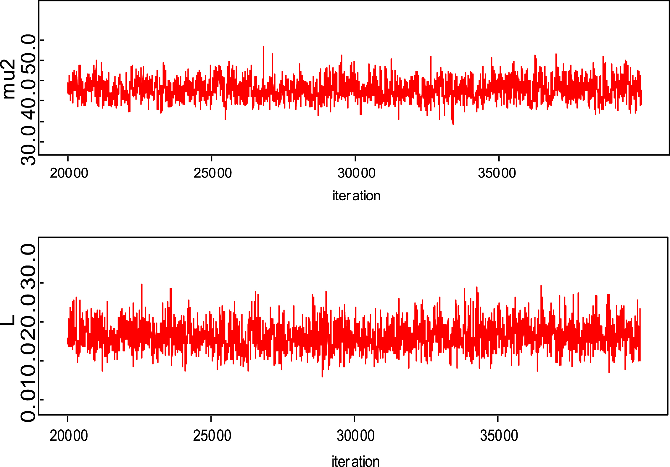
Bayesian analysis of the model described in section 4 is undertaken in OpenBUGS software. Bayes estimates are obtained through posterior distributions which are in form of complex integrals and difficult to compute without computing. Smith & Gelfand,1993 showed that simulation can be used to draw samples from such complex integrals. Metropolis et al., 1953 and Hastings, 1990 developed Markov Chain Monte Carlo (MCMC) algorithms which iteratively produced sequential samples of dependent draws. The dependency appears as autocorrelation since the long stream of numbers are generated from a Markov Chain (Spiegelhalter et al., 1996). MCMC simulated chains converge to the desired posterior distribution. In the present work MCMC algorithm is utilised to simulate 20,000 data points out of which the initial 2000 generated data points are discarded as burn-in to make dependency in the posterior samples redundant. Such trimmed samples are then aggregated to obtain posterior summaries. Box-plots based on posterior summaries for effective batting average, mi for each player is plotted in Figs. 6–11. Box plot represent the dispersion in the value of effective batting average obtained through equation (1) and (2) for each inning of batsman estimated under Bayesian setup. Effective batting average for each inning can be given as posterior mean like we have presented for components (μ1, μ2and L) of effective batting average in Table 2 but in order to represent the dispersion in MCMC generated posterior sample values for effective batting average and to reflect on batsman’s consistency through number of innings in which effective batting average remains above combined effective batting average of all the innings represented by central line authors presented box-plots instead of mean of posterior sample. Posterior summary for all components of effective batting average (mi) i.e., μ1, μ2and L are obtained and presented in Table 2. Performance analysis of each batsman is demarcated by posterior mean and posterior probabilities. It is evident from Table 2 that Shreyas Iyer leading with highest estimated values for μ1 and μ2 Posterior mean and probability for L<20 is higher for Rishabh Pant and Dinesh Kartik indicating that these batsmen get less number runs to get their ‘eye-in’ and play their shots with highest ability. Posterior density and trace plots are shown in Figs. 12 and 13, respectively. Density plots and trace plots are diagnostic tools for detecting convergence in generated MCMC sample for the parameter under interest. If the shape of the density plot is bell curved and distribution is unimodal then the parameter under interest is said to achieve convergence. Convergence diagnostics for MCMC generated samples for the parameters under interests adopted are well utilised from OpenBUGS software (https://www.mrc-bsu.cam.ac.uk/wp-content/uploads/2021/06/OpenBUGS_Manual.pdf).
Fig. 6
Box plot of Ajinkya Rahane’s effective average mi.
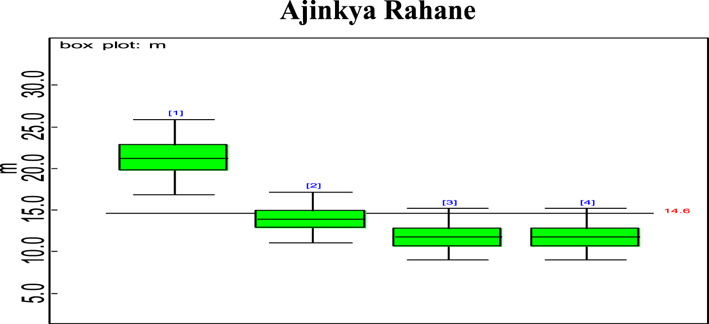
Fig. 7
Box plot of Ambati Raydu’s effective average mi.
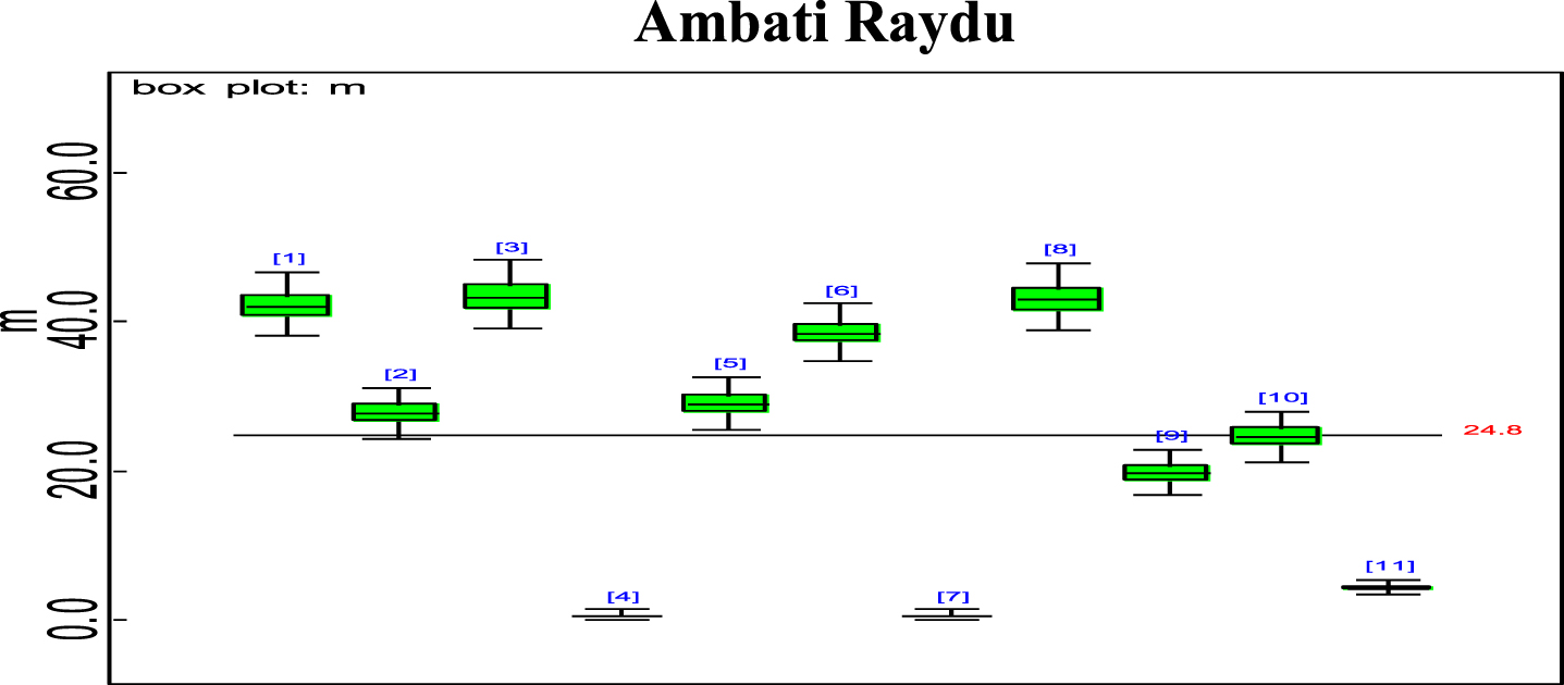
Fig. 8
Box plot of Shreyas Iyer’s effective average mi.
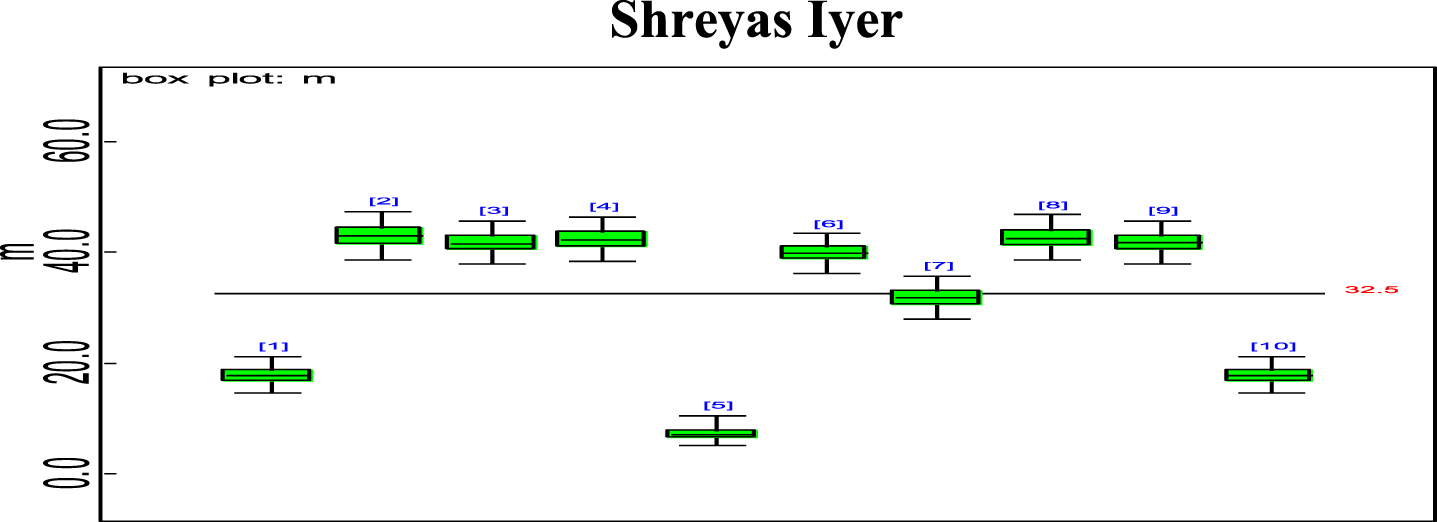
Fig. 9
Box plot of Rishabh Pant’s effective average mi.
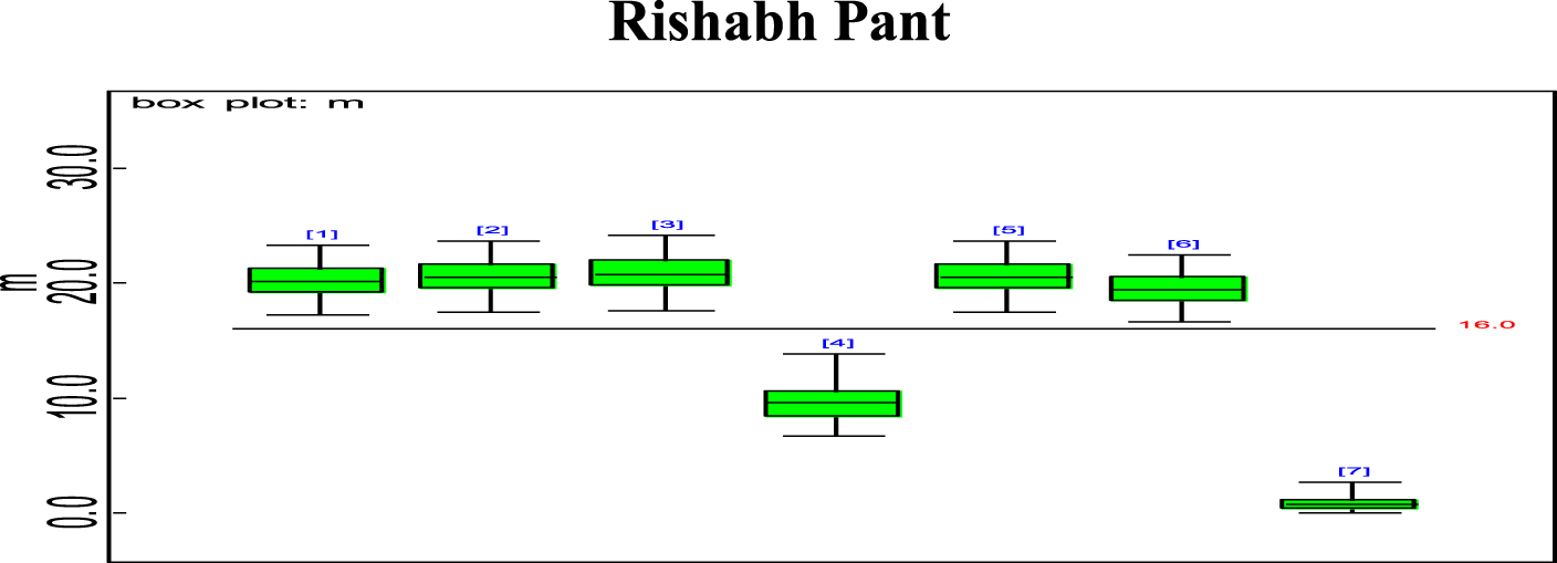
Fig. 10
Box plot of KL Rahul’s estimated effective average mi.
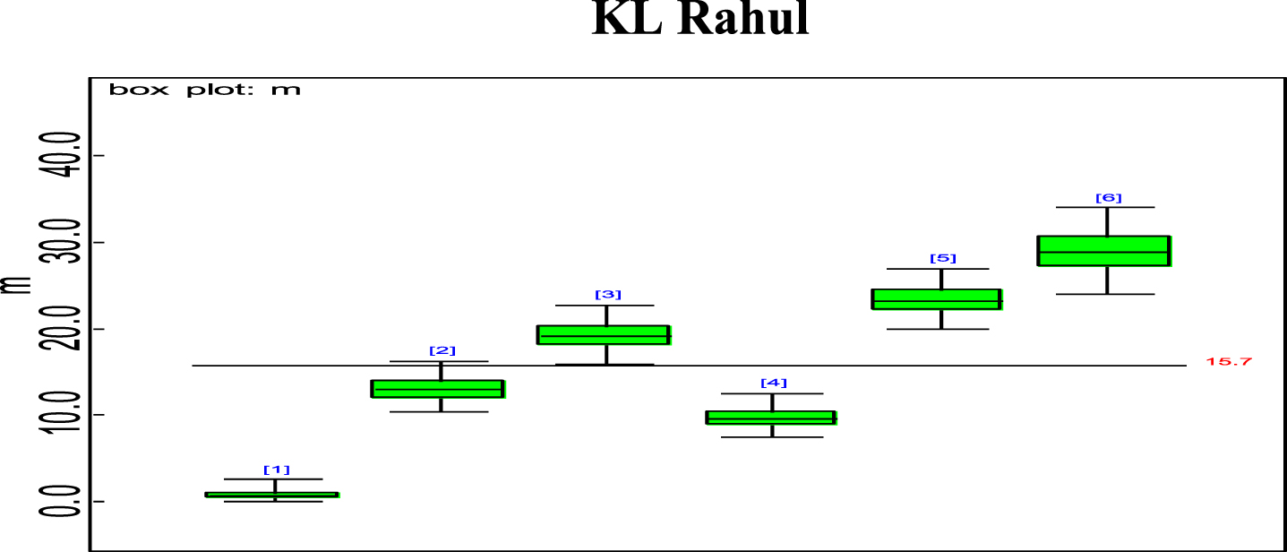
Fig. 11
Box plot of Dinesh Kartik’s estimated effective average mi.
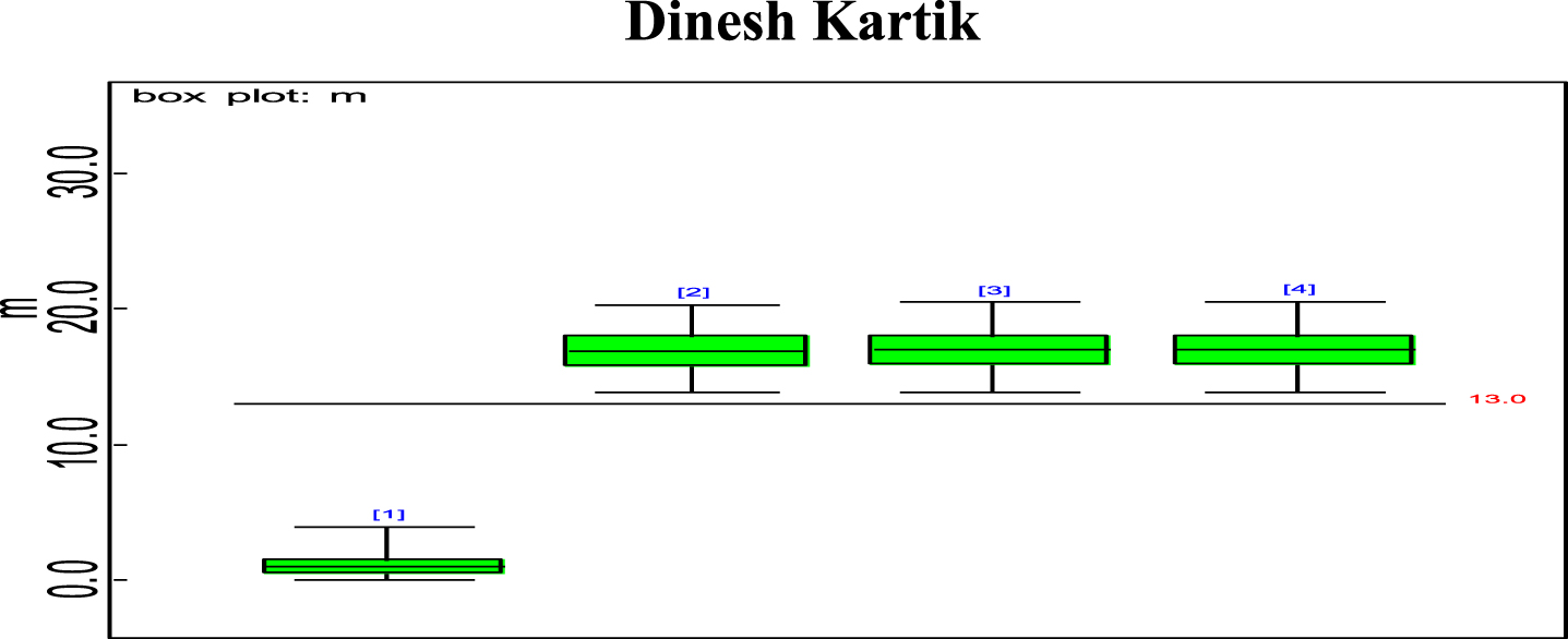
Fig. 12
Density plots.
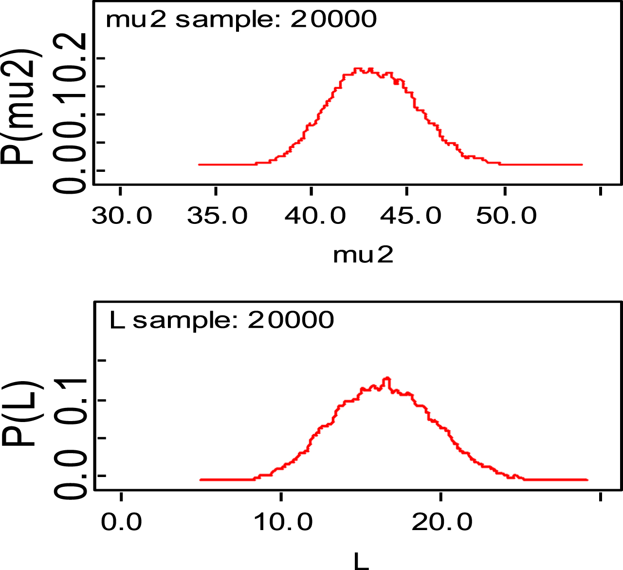
Fig. 13
Trace plots.
6Discussion and conclusion
Cricket fraternity comprises of different experts each of whom have a distinct analysis strategy for the outcomes of matches based on their individual logic. Cricket is game of uncertainties and dynamics of a particular game changes very rapidly which also depend on the form of players on a particular match day. Selectors pick players in TI considering their performance in domestic cricket and in Indian Premier League (IPL). It is always difficult for captain and team management to drop or pick when there is close competition among two players. Here, we present a statistical approach which gives an unbiased opinion on comparison of performances for closely competing players. This analytic approach might augment the existing selection strategies utilised by the cricket analytic experts to support selection committee of Board of Cricket for Control in India (BCCI).
The present paper proposes a simple survival analysis approach which allows analysis of individual and pairwise player-assessment at a time (Fig. 1–Fig. 5). Such an assessment, undertaken for the first time in sports related research, enables quantification of how players’ abilities differ, taking into account the fact that the information about any player is limited by the finite number of innings that they have played.
Also, Bayesian modelling approach is adopted for analysing initial and final playing abilities of a group of Indian batsmen who have played at the fourth position for team India in ODI cricket. Table 2 represents posterior estimates which reveals Shreyas Iyer to have highest BPA. Criteria for comparison and selection of N4 batsman is based on the final batting average ′m2′ which is the indicator of best playing ability of a batsman. Another important indicator i.e., number of runs required to transit from initial playing ability to final or best playing ability is the e-folding time ‘L’ which is used for performance ranking whenever two batsmen show a tie on the final batting average. The latter one will be more relevant criteria of comparison in case of shorter formats like T20s. The present analysis for ODIs show that Shreyas Iyer has the best final batting average and so is the corresponding posterior probability. As far as future scope for this research is concerned, we can assess performance of different batsman in T20’s by setting up threshold of 30 runs and 10 runs for μ2 and L, respectively.
The present work proposes modelling for runs scored in a ODI by an Individual batsman who have potential to sustain themselves for longer period on the field, in pursuit of devising strategies for selection of the right players in the middle order batting position. Initial playing ability is the intensity with which batsman plays when he first arrives at the crease and is shy of playing his shots and is sometimes tentative because gets beaten by the swing offered by the fast bowlers and tries to adjust the pace, bounce and turn offered by the pitch. Therefore, we are able to see the low posterior estimates (Table 2) for initial playing ability. Adapting quickly to pitch conditions and understanding the opposition plan of attacking are the key to get your ‘eye-in’ quickly and score runs. Such an adaption of batsman is quantified in the present research which analyses the performance of batsman playing ability fragmented into three parts i.e., initial playing ability, final playing ability and the transition time between the two through adopted Bayesian model. Box-plots for effective batting average, mi, of individual player’s innings (Fig. 6–Fig. 11) represents variation in batting performance or consistency of the batsman. Also, box plots indicate how many times out of total innings considered for a batsman, he had played above the combined posterior mean of his effective batting average. Shreyas Iyer, Rishabh Pant and Dinesh Kartik are observed to be more consistent and their effective average of individual innings remains above combined effective batting average of all the innings played.
Acknowledgments
Authors express their gratitude to all the anonymous reviewers and the editor for their constructive comments and suggestions which resulted in immense improvement in the original manuscript.
References
1 | Basu, D ,(1988) , Statistical Information and Likelihood. J. K. Ghosh (ed.),Springer-Verlag, New York. |
2 | Bracewell, P.J , Ruggiero K , (2009) , A parametric control chart for monitoring individual batting performances in cricket, Journal of Quantitative Analysis in Sports, 5: (3). |
3 | Brewer, B.J , 2008, Getting your eye in: A Bayesian analysis of early dismissals in cricket. arXiv preprint arXiv:0801.4408. |
4 | Clarke, S.R , (1988) , Dynamic programming in one-day cricket-optimal scoring rates, Journal of the Operational Research Society 39: (4), 331–337. |
5 | Clarke, S.R , Norman, J.M , (1999) , To run or not?: Some dynamic programming models in cricket, Journal of the Operational Research Society 50: (5), 536–545. |
6 | Clarke, S.R , Norman, J.M , (2003) , Dynamic programming in cricket: Choosing a night watchman, Journal of the Operational Research Society 54: (8), 838–845. |
7 | Cai, T , Hyndman R.J , Wand M.P . (2002) , Mixed model-based hazard estimation, Journal of Computational and Graphical Statistics 11: (4), 784–798. |
8 | Damodaran, U , (2006) , Stochastic Dominance and Analysis of ODI Batting Performance: The Indian Cricket Team 1989–2005, Journal of Sports Science and Medicine 5: , 503–508. |
9 | Davis, J , Perera, H , Swartz, T.B . (2015) , Player evaluation in Twenty cricket, Journal of Sports Analytics 1: (1), 19–31. |
10 | Elderton W , Wood G.H , (1945) , Cricket scores and geometrical progression, Journal of the Royal Statistical Society, 108: (1/2), 12–40. |
11 | Gelman, A , Price P.N , (1999) , All maps of parameter estimates are misleading, Statistics in Medicine 18: (23), 3221–3234. |
12 | Haining R.P , Law J , 2011 Geographical information systems models and spatial data analysis (pp. 377-401). World Scientific Publishing Co. Pt. Ltd. |
13 | Hastings, W.K , (1970) , Monte Carlo Sampling Methods using Markov Chains and their Applications, Biometrika 57: , 97–109. |
14 | Jayalath, K.P , (2018) , A machine learning approach to analyze ODI cricket predictors, Journal of Sports Analytics 4: (1), 73–84. |
15 | Kaplan E.L , Meier P , (1958) , Nonparametric estimation from incomplete observations, Journal of the American Statistical Association 53: (282), 457–481. |
16 | Kimber A.C , Hansford A.R , (1993) , A statistical analysis of batting in cricket, Journal of the Royal Statistical Society: Series A (Statistics in Society) 156: (3), 443–455. |
17 | Koulis T , Muthukumarana S , Briercliffe C.D (2014) , A Bayesian stochastic model for batting performance evaluation in one-day cricket, Journal of Quantitative Analysis in Sports 10: (1), 1–13. |
18 | Lee E.T , Wang J , (2003) , Statistical methods for survival data analysis (Vol. 476).John Wiley & Sons. |
19 | Metropolis N , Rosenbluth A.W , Rosenbluth M.N , Teller A.H , Teller E , (1953) , Equation of state calculations by fast computing machines, J Chem Phys 21: , 1087–1092. |
20 | Norman J.M , Clarke S.R , (2010) , Optimal batting orders in cricket, Journal of the Operational Research Society 61: (6), 980–986. |
21 | Preston I , Thomas J , (2000) , Batting strategy in limited overs cricket, Journal of the Royal Statistical Society: Series D (The Statistician) 49: (1), 95–106. |
22 | Robert C.P , (2001) , The Bayesian Choice. Springer-Verlag, New York.. |
23 | Smith A.F.M , Gelfand A , (1993) , Bayesian Statistics without tears, American Statistician 46,: 84–88. |
24 | Spiegelhalter D , Thomas A , Best N , Gilks W , 1996, BUGS 0.5: Bayesian inference using Gibbs sampling manual (version ii). MRC Biostatistics Unit, Institute of Public Health, Cambridge, UK, 1-59. |
25 | Stevenson O.G , Brewer B.J , (2017) , Bayesian survival analysis of batsmen in Test cricket, Journal of Quantitative Analysis in Sports 13: (1), 25–36. |
26 | Swartz T.B , Gill P.S , Muthukumarana S , (2009) , Modelling and simulation for one-day cricket, Canadian Journal of Statistics 37: (2), 143–160. |
27 | Zellner A , (1995) , Bayesian and non-Bayesian approaches to statistical inference and decision-making, Journal of Computational and Applied Mathematics 64: (1-2), 3–10. |


