
Putting team formations in association football into context
Abstract
Choosing the right formation is one of the coach’s most important decisions in football. Teams change formation dynamically throughout matches to achieve their immediate objective: to retain possession, progress the ball up-field and create (or prevent) goal-scoring opportunities. In this work we identify the unique formations used by teams in distinct phases of play in a large sample of tracking data. This we achieve in two steps: first, we train a convolutional neural network to decompose each game into non-overlapping segments and classify these segments into phases with an average F1-score of 0.76. We then measure and contextualize unique formations used in each distinct phase of play. While conventional discussion tends to reduce team formations over an entire match to a single three-digit code (e.g. 4-4-2; 4 defender, 4 midfielder, 2 striker), we provide an objective representation of team formations per phase of play. Using the most frequently occurring phases of play, mid-block, we identify and contextualize six unique formations. A long-term analysis in the German Bundesliga allows us to quantify the efficiency of each formation, and to present a helpful scouting tool to identify how well a coach’s preferred playing style is suited to a potential club.
1Introduction
The great Dutch football player Johan Cruyff famously observed that, on average, each player is in possession of the ball for only 3 of the 90 minutes during a football match.1 He expanded on this observation by stating “... so, the most important thing is: what do you do during those 87 minutes when you do not have the ball? That is what determines whether you are a good player or not.” 2 The implication is that a player can significantly influence the game through their positioning and movement on the field, even when they do not directly interact with the ball (Brefeld et al., 2019; Fernandez et al., 2018).
The movement of players in a football match represent a high-dimensional spatio-temporal configuration. Various studies have attempted to encode team-level behavior. Balague et al. (2013) focuses on coordination of motion within a team by modelling a team’s movement as collective behavior in a complex system, and synchronicity of movements is investigated in football in specific situations (Goes et al., 2020b; Sarmento et al., 2018). Several studies described football matches as multi-agent systems (Beetz et al., 2006; Fujii, 2021) highlighting the intelligence of interactions between the agents (players). Analysing movement patterns in spatio-temporal data, especially the detection of repeating, collective patterns is not only researched in invasion sports (Gudmundsson et al., 2017a), but also in traffic management, surveillance and security or in the military and battlefield domain (Gudmundsson et al., 2017b). Key challenges in spatio-temporal pattern detection are: (a) Using the interaction of movement for dimensional reduction (Balague et al., 2013), (b) finding appropriate similarity metrics for related, but never identical trajectories of multiple entities (Vilar et al., 2013), and (c) projecting multi-agents in a permutation-invariant space (Bauer et al., 2022; Anzer et al., 2022b; Bauer, 2021; Yeh et al., 2019).
The literature differentiates between tactics (decisions made during a match as a consequence of the dynamic interaction in a match) and strategy (decisions made before the match) (Gráhaigne et al., 1999). However, these concepts are often hard to distinguish (Rein et al., 2016). Coming from a more general understanding of team formations (Wang et al., 2015), Budak et al. (2019) highlighted the problem of optimizing the team composition (i.e. which players should be on the pitch) before the season, before the match and during the match stage as a relevant problem in team sports. According to this definition, several approaches presented evidence-based strategies to optimize this composition of players (Boon et al., 2003). However, this neglects the players interaction on the pitch (i.e. tactics), which is the focus of our investigation and will henceforth be generally referred to as the (playing) formation.
For the longest time one could not objectively measure a team’s playing formation, since the only available data describing football matches was so-called event data. Dating as far back as 1968 when Charles Reep started manually collecting events such as shots or passes (Reep et al., 1968), this event data, which is still being manually collected today, describes all ball actions and the players involved (Pappalardo et al., 2019b; Stein et al., 2017). Although event data allowed for ground-breaking discoveries in football tactics (Xu, 2021; Pantzalis et al., 2020; Decroos et al., 2019; Danisik et al., 2018; Decroos et al., 2018; Pappalardo et al., 2019a; Cintia et al., 2015; Haaren et al., 2013), it does not include any information about the positioning of all other players. Now, with recent developments in computer vision technologies (Thinh et al., 2019; Baysal et al., 2016; Teoldo et al., 2009) it has become possible to capture exactly that: optical tracking systems are able to record centimeter-accurate positions of all players at every moment of a match (hereafter referred to as positional or tracking data). This development unlocked huge potentials for professional football (Rein et al., 2016; Anzer et al., 2022a, 2021a; Araújo et al., 2021; Wang et al., 2020; Goes et al., 2020a; Andrienko et al., 2019; Herold et al., 2019).
The first approaches in football analysed formations assuming that teams play with a fixed formation across the whole match, describing them simply as playing with a 4-4-2 (4 defenders, 4 midfielders and 2 forwards), 5-3-2, 4-3-3, or one of approximately ten other formations that are commonly referenced (Wilson, 2009). Differences in physical requirements for similar player-roles in different formation (e.g. a central defender in a 4-4-2 versus a 5-4-1) were analysed (Vilamitjana et al., 2021; Tierney et al., 2016; Carling, 2011; Bradley et al., 2011). However, breaking a team’s formation down to three digits in a complex sport like football is a gross over-simplification (Müller-Budack et al., 2019).
Driven by the increasing availability of tracking data, analysing team formations has been a research issue in several sports (Gudmundsson et al., 2017b). Initiated by a pioneering work in 1999 (Intille et al., 1999), unique formations were derived at the moment a play starts using positional data in American football (Atmosukarto et al., 2013). Hochstedler et al. (2017) build on the static formation detection in American football by classifying the routes of chosen player during the plays. In basketball, event data has been used to investigate established player roles (Bianchi et al., 2017). Lucey et al. (2013) published a quantitative analyses of team formations in field-hockey using tracking data, which was transferred to football (Wei et al., 2013) and incrementally extended (Bialkowski et al. (2014b, 2015), Bialkowski et al. (2016)). They describe formations as a “a coarse spatial structure which the players maintain over the course of the match” and which assigns each player at every time of the match a unique role. Bialkowski et al. (2015) further define a role as a players position relative to the other roles. They describe a role-identification methodology for measuring formations, iteratively refining estimates of the average spatial positions (and deviations from those positions) of ten unique outfield roles throughout a match. Applying a clustering algorithm on tracking data for a season of a 20-team professional league, Bialkowski et al. (2014b) identified six unique formation types: for example 4-4-2, 3-4-3, 4-4-1-1 and 4-1-4-1 are all visible in their results. Variations in formations between game-states (i.e. offensive, defensive) were first explored in Bialkowski et al. (2016). Using a more supervised approach, Müller-Budack et al. (2019) annotated twelve typical formations (split between offense and defense) and addressed the formation problem as a classification task. Narizuka et al. (2019) derived unique formations of 45 Japanese J1 league using a Delaunay method combined with hierarchical clustering.
Ric et al. (2021) and Shaw et al. (2019) presented a data-driven technique for measuring and classifying team formations as a function of game-state (offensive, defensive, transition), analysing the offensive and defensive configurations of each team separately and dynamically detecting major tactical changes during the course of a match. Defensive and offensive formations were measured separately by aggregating together consecutive periods of possession of the ball for each team into two-minute windows of in-play data. Splitting up formations into different game-states, i.e. excluding fuzzy transition situations, presented a major improvement of formation analysis, however, they stated that further sub-game-states should be considered in future work to achieve even more granularity (Ric et al., 2021).
While these pioneering studies have provided methods for measuring team formations and demonstrated observations of the coherent structures formed by teams as they move around the field (and validated by football experts), they do not fully account for the changing objectives of a football team as a match evolves, influencing team formations drastically (Gudmundsson et al., 2017b; Andrienko et al., 2019; Lucey et al., 2013; Bialkowski et al., 2016; Shaw et al., 2019). Several studies have pointed out that football consists of repetitive movement patterns that can be recognized by experts (Sampaio et al., 2012). We define a tactical pattern as a recurring, collective behavior conducted by a team, or a sub-group of a team in a specific situation of a match, that can be clearly identified by experts (Rein et al., 2016; Wang et al., 2015; Kempe et al., 2015; Grunz et al., 2012).
Whereas the detection of tactical patterns has been a relevant issue in basketball (Kempe et al., 2015; Chen et al., 2014; Perse et al., 2006), handball (Pfeiffer et al., 2015), American football (Hochstedler et al., 2017; Stracuzzi et al., 2011; Li et al., 2010; Siddiquie et al., 2009), and Australian rules football (Alexander et al., 2019), often only patterns conducted by subgroups of players are analysed. The complexity of a football match requires so called team tactics in which the whole team is involved (Rein et al., 2016). Some exemplary patterns like counterattacks (Fassmeyer et al., 2021; Hobbs et al., 2018), ball regain strategies (Vogelbein et al., 2014), i.e. counterpressing (Bauer et al., 2021), or general offensive strategies (Decroos et al., 2018; Grunz et al., 2012; Kempe et al., 2014; Borrie et al., 2002; Montoliu et al., 2015; Fernando et al., 2015) have been addressed in literature and classified as sub-categories of game-states (e.g. counterattacks and counterpressing as a subgroup of transitions in Hobbs et al. (2018) and Bauer et al. (2021)). For such well-established tactical patterns, which unavoidably occur in every match, practitioners often use the term phases of play 3 (although no scientific definition established) or game-phases (Lucey et al., 2014).
The consequence of this is that the results are not observations of a single distinct formation of a team, but a mixture (or ‘superposition’) of the different formations used in different phases of play (Müller-Budack et al., 2019; Shaw et al., 2019). This paper resolves this problem by using a convolutional neural network (CNN) to classify a football match over time into distinct phases of play, before measuring the formations used by either team in each distinct phase. There are therefore two parts to our approach:
(1) A phases of play detection CNN, with architecture specifically designed for the purpose, was trained using labeled tracking data from 97 matches in the German Bundesliga based on phases of play classifications provided by professional analysts. Our classification scheme is described in Section 3.
(2) Within each match, periods of play classified to the same phases of play (from the perspective of one team) are then aggregated to obtain precise measurements of the formations used. This is described in Section 4.
We apply the phases of play classifier and formation measurement tools to tracking data obtained for 2142 matches in the German Bundesliga over seven seasons, identifying the unique formations used in each phase of play across our sample. This combination of a phase of play detection and formation detection fully automates the process of identifying the distinct formation configurations used by teams during a game, revealing the specific instructions that managers gave their team. This research was conducted in close collaboration with professional match analysts from German Bundesliga clubs and the German national teams, who have provided human validation of our methodology and results. The project therefore combines machine learning and human experience aiming to obtain results that are insightful, meaningful and of practical use to coaches, managers, and scouts.
As a side-product of a practical relevant process automatization for match analysis departments, we outline two clear use-cases of our work in Sec. 5. We are the first to quantify the strengths and weaknesses of a specific formation when pitted against another, providing the foundation for evidence-based advice for managers seeking the most effective counter to an opponent’s strategy during specific phases of the game (Sec. 5.1). Second, we assess the tactical preferences of individual managers, highlighting how our tools can be used to find managers that would provide continuity to a team’s existing playing style (Sec. 5.2). Style-matching is a crucial element of managerial recruitment, helping to prevent a large turnover of players as a manager seeks to impose a new playing style on a new team.
2Positional data
The German Bundesliga collects consistent positional data on a league-wide level, making this data available to every team. Positional data, often also referred to as tracking or movement data (Stein et al., 2017), contains measurements of the positions of all players, referees, and the ball, sampled at a frequency of 25 Hz. This data is gathered by an optical tracking system that captures high resolution video footage from different camera perspectives.
In this paper, we make use of positional data from seven seasons of the German Bundesliga, from 2013/2014 until 2019/2020: a total of 2,142 matches and nearly half a billion frames are acquired by Chryronhego’s TRACAB system.4 Validating the quality of such tracking data presents somehow an ill-posed problem due to missing ground truth positions. Even though, several studies evaluated the accuracy of the underlying data used in this study (Redwood-Brown et al., 2012; Linke et al., 2018; 2020; Taberner et al., 2020), and found an average diversion of less than 10cm for player positioning compared to an accurate measurement system. Pettersen et al. (2014) presents a publicly available set of positional data, which can be used for reproduction.5
3Phases of play classification
3.1Defining phases of play
The primary goal in football is to score more goals than the respective opponent. Consequently, the two major objectives are scoring goals and preventing the opponent from doing so (Kempe et al., 2014). However, given specific situations those goals are often only implicitly followed, while sub-tasks (e.g. (re)gaining possession of the ball), are predominant in certain situations. The concept of phases of play derives from the idea that any moment of a match can be categorized based on the immediate intentions of each team, e.g. in defense, teams always have to balance between the two most relevant objectives of regaining the ball (preferably in a good position to perform an attack) and purely prevent the opponent from scoring. At the simplest level, a match can be divided into the phases of offense and defense for each team (António et al., 2014), i.e., periods in and out of possession of the ball. At a more granular level, professional analysts involved in our project classified the progressive stages of attacking and defense into distinct phases.6 Figure 1 provides an example of the phases of play classification scheme developed by German Bundesliga analysts. In this scheme, open-play during a match revolves between periods of offense, transition to defense, defense, and transition to offense, with set-pieces providing a separate category (which could also be broken further down into offensive and defensive set-pieces as well as different categories such as corner kicks, throw-ins and freekicks).
Fig. 1
Overview of tactical phases of play considered.
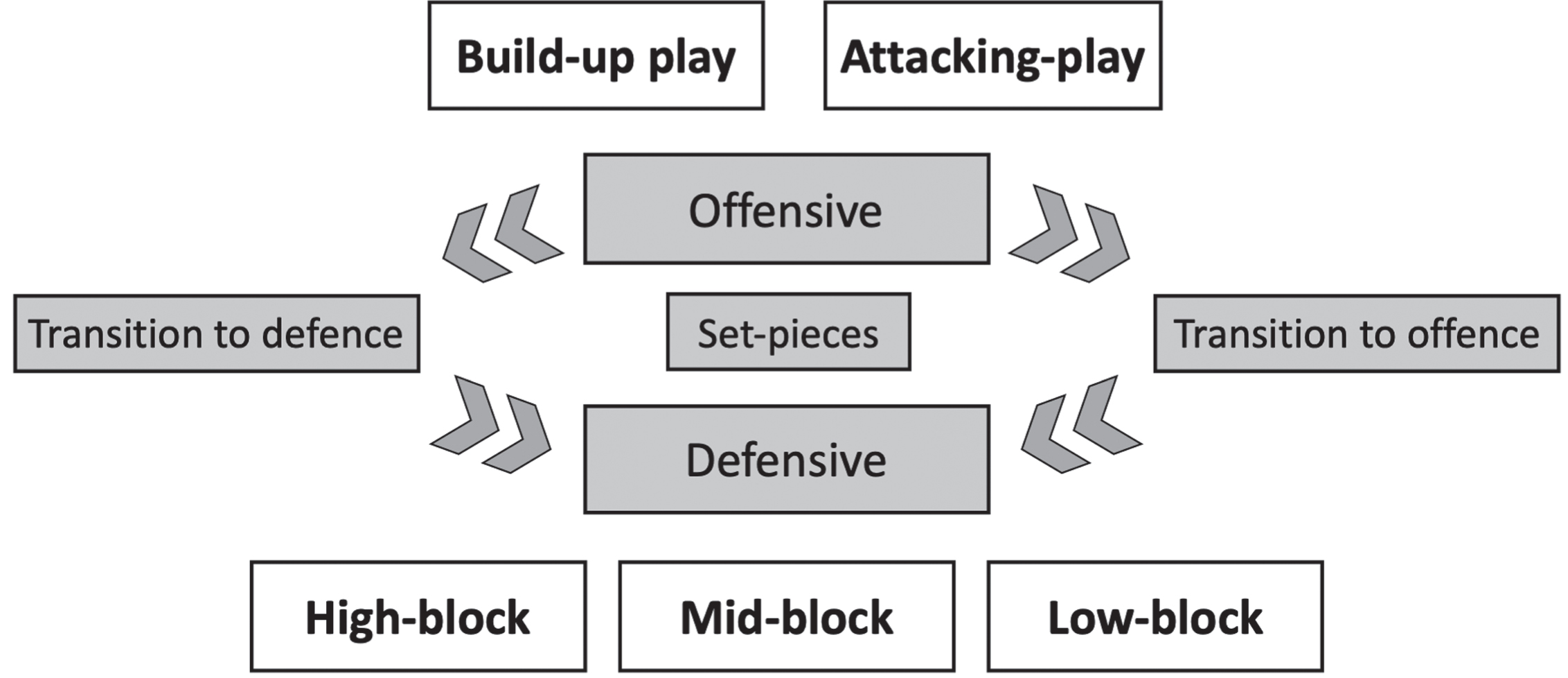
Offensive play is divided into two phases: build-up, where the objective is to breach the opponent’s first defensive line, and attacking-play, where the first line of defenders has been outplayed and the main objective is to create a goal-scoring opportunity. In defense, professional analysts differentiate between aggressive attempts to reclaim possession near the opponent’s goal (high-block), a default defensive stance as the opponent progresses the ball up the field (midfield-block or mid-block) and a very compact defensive stance near to a team’s own goal, where the sole objective is to prevent the opponent from scoring (low-block). These defensive phases were also explored in Anzer et al. (2021b) and Power et al. (2017).
Figure 2 shows the phases of play break-down of a two-minute sequence of play during the Nations League match between the German men’s national team and Spain in September 2020. The central plot shows the distance between the German team centroid (the average position of the outfield players) and their own goal from the 36th to 38th minutes of the game. The highlighted regions indicate the phases of play classifications, from the perspective of the German team, as determined by professional German match analysts. Freeze frames from the footage are shown at four different instants.
Fig. 2
Team behavior per phase of play by the reference of Germany against Spain (3rd of September 2020, venue: Stuttgart, result: 1:1). The highlighted areas (red) in the video-footage mark the current ball action.
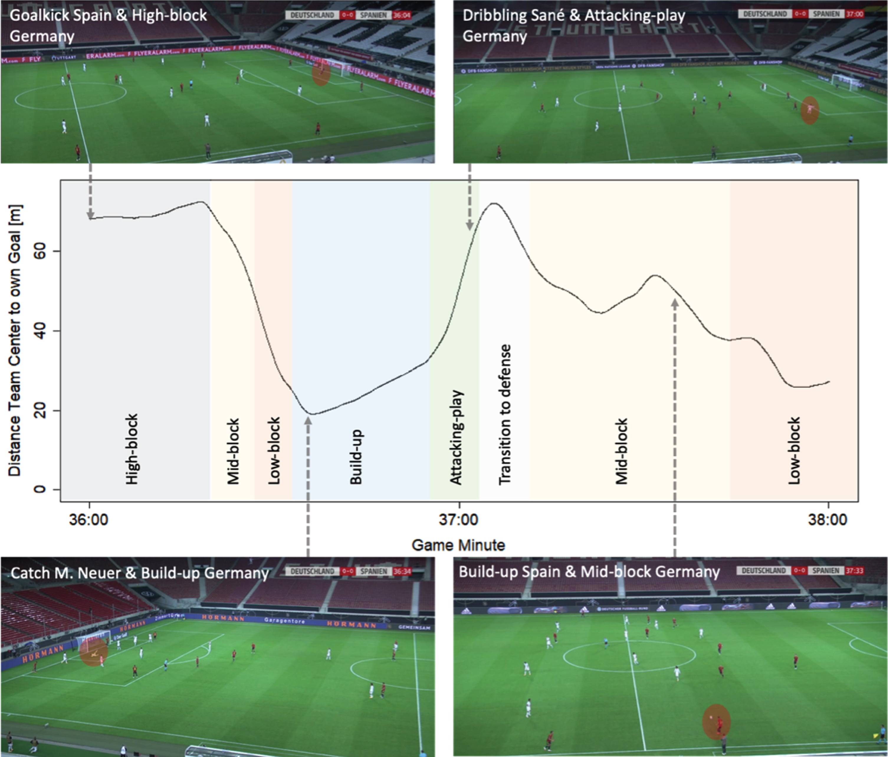
The passage of play starts with a Spanish goal kick. Germany confronted this situation by attempting to force a turnover near to the Spanish goal with a high-block. Over the first 30 seconds of play, the Spanish team played through the high-block, forcing Germany to retreat, first into a mid-block and then to a low-block to defend their own goal. Germany regained possession after a shot saved by Manuel Neuer (Germany’s goalkeeper) and immediately initiated a build-up phase of possession. A long pass towards Leroy Sané on the right side of the field briefly brought Germany into the attacking-play phase. However, Spain rapidly won the ball back, after which Germany transitioned into a defensive mid-block and then a low-block as Spain advanced again.
Match analysts spend a substantial proportion of their time manually breaking down and classifying matches into tactical phases by watching video footage. There are very few methods published in the literature that attempt to automate this process. Those that do focus on finding a single specific transition phases, such as counterattacking (Decroos et al., 2018; Fassmeyer et al., 2021; Hobbs et al., 2018) or counterpressing (Bauer et al., 2021), but none attempt to classifying entire games. We now describe our methodology for achieving this.
3.2Automated detection of phases of play
The phases of play definitions shown in Fig. 1 were established in collaboration with professional match analysts from Bundesliga teams. These definitions were then adopted by professional match analysts to annotate 97 Bundesliga matches from the 2018/2019 season. In order to evaluate the inter-labeller reliability, 20 of these matches were independently annotated by three different labelleres and the pairwise accuracy (calculated frame-by-frame) is shown in Table 2 for each phase. For the final model training, the label of the 20 matches annotated by multiple experts was decided by a majority vote and the remaining 77 matches were only annotated once. The annotated data consists of the first eleven matchdays of the Bundesliga 2018/2019 season— labelling was always conducted from the perspective of the home team. Using the expert-labelled matches as a training set, we explored two different machine learning approaches for automated classification of phases of play using optical tracking data.
The first approach is a rule-based baseline model, as described in Table 1; the results of the prediction of the rule-based approach (compared to the inter-labeller accordance) are shown in row four in Table 2.
The second approach makes use of convolutional neural networks (CNN), which enables us to model spatio-temporal football data in a high dimensional, permutation-invariant space (see also Dick et al. (2019), Zheng et al. (2016), and Wang et al. (2016)), using the raw positional data as input instead of requiring a costly step of feature engineering (as conducted in Bauer et al. (2021) to detect counterpressing as another example of a tactical pattern). For CNN, the positional data is mapped to 2-D images. For training, we split the labeled data into 75% training and 25% test data. On the training data we used a Bayesian hyper-parameter optimization and a 5-fold cross-validation. Further details regarding the network architecture can be found in the Appendix A.
Table 1
Rules for baseline model formation detection
| Phase of play | Rule |
| Offensive | The first 6 seconds after a team gains ball possession are classified as transition to offense. The remaining time during a ball possession are classified as the offensive phase. |
| Build-up | Any moment during the offensive phase, when the ball is within its own third or the mid third of the pitch is classified as build-up. |
| Attacking-play | Any moment during the offensive phase, when the ball is within the opponents third is classified as attacking-play. |
| Defensive | The first 6 seconds after a team loses ball possession are classified as transition to defense. The remaining time during a ball possession are classified as the defensive phase. |
| Low-block | Any moment during the defensive phase, when the defending team’s center (of the outfield players) is at most 20 meters from its own goal-line, is classified as low-block. |
| Mid-block | Any moment during the defensive phase, when the defending team’s center (of the outfield players) is between 20 meters and 60 meters from its own goal-line, is classified as mid-block. |
| High-block | Any moment during the defensive phase, when the defending team’s center (of the outfield players) is at further than 60 meters from its own goal-line, is classified as high-block. |
On a frame-by-frame level, the CNN predicts the phases of play in our test set with a weighted average F1 score, the harmonic mean of recall and precision (see also Goutte et al. (2005)), i.e. the mean of all per class F1-scores weighted by their frequency of 0.76, which is basically limited by the frame-by-frame pairwise inter-labeller reliability (i.e. the pairwise accuracy for the 20 matches annotated by all three experts) of 85% (weighted F1-score of 0.72) and exceeds the accuracy of the baseline model (0.69). On further examination, we found that the mis-classified frames mainly occurred near the start and end points of each phase of play.
Table 2 shows some basic statistics for the training data, including the F1-score.
Table 2
Outcome of the phases of play detection CNN
| Tactical phase of play | Low-block | Mid-block | High-block | Build-up | Attacking-play |
| Labeled phases | 1h 57min | 23h 30min | 1h 53min | 27h 37min | 4h 53min |
| (3 %) | (39 %) | (3 %) | (47 %) | (7 %) | |
| Average duration | 9.1s | 19.0s | 13.3s | 18.6s | 8.1s |
| F1-score | 0.37 | 0.80 | 0.29 | 0.83 | 0.54 |
| Baseline model F1-score | 0.18 | 0.75 | 0.26 | 0.76 | 0.39 |
| Inter-labeller reliability (avg. F1-score) | 0.38 | 0.78 | 0.24 | 0.79 | 0.45 |
Mid-block and build-up are clearly the dominant phases, making up 39% and 47% of the phases shown in Table 2. They are also the phases with the longest duration, lasting an average of 19.0 seconds (mid-block) and 18.6 seconds (build-up). As the mid-block is the standard opponent response to the build-up phase, it is not surprising that the average durations are similar in length. These phases also have the highest classification accuracy for our CNN, with both having F1-scores exceeding 0.8. The next most regular phase is attacking-play, making up 7% of the training data. Low-block (3%) and high-block (3%) are the least frequently occurring phases. For these phases the model exhibits lower F1-scores, but still outperforms the rule-based model.
The trained model was applied on seven full seasons of German Bundesliga (2013/2014-2019/2020). Much of the following analysis focuses on the two most frequent phases: build-up and mid-block.
4Formation detection
4.1Phase-dependent formations
Although positional data has been used in recent literature to quantify team-formations (Müller-Budack et al., 2019; Wei et al., 2013; Bialkowski et al., 2015; Bialkowski et al., 2016; Shaw et al., 2019; Bialkowski et al., 2014a), they aggregate player positions over the entire match ignoring tactical changes during the match. In the following we motivate the relevance of a more granular contemplation.
Figure 3 shows the different formations employed across each of the five phases of play for one team during a Bundesliga match (data are used only until the first substitution). The dots indicate the average position of each player in the formation; the ellipses provide an estimate of how far players tend to move from their average positions (the team is playing from left to right), visualized through their 80% confidence region. A wider ellipsis around a player does not necessarily imply that the player is moving more but instead that his positioning has a wider variance respective to his team center, defined as the average position of all outfield players of his team for any given time-point as in Bourbousson et al. (2010) and Andrienko et al. (2017). The lower three images show the formations in the three defensive phases: low-block (left), mid-block (center) and high-block (right); the top images show the formation in the two offensive phases: build-up (left) and offense (right).
Fig. 3
Average player positions of a team per tactical phase of play during one match. The ellipses provide an estimate of how far the player would tend to move from their average position during each phase of play. The considered team plays from left to right. Player’s positions are collected by optical tracking systems at 25 Hz (positional data). For this figure only data until the first substitution was used.
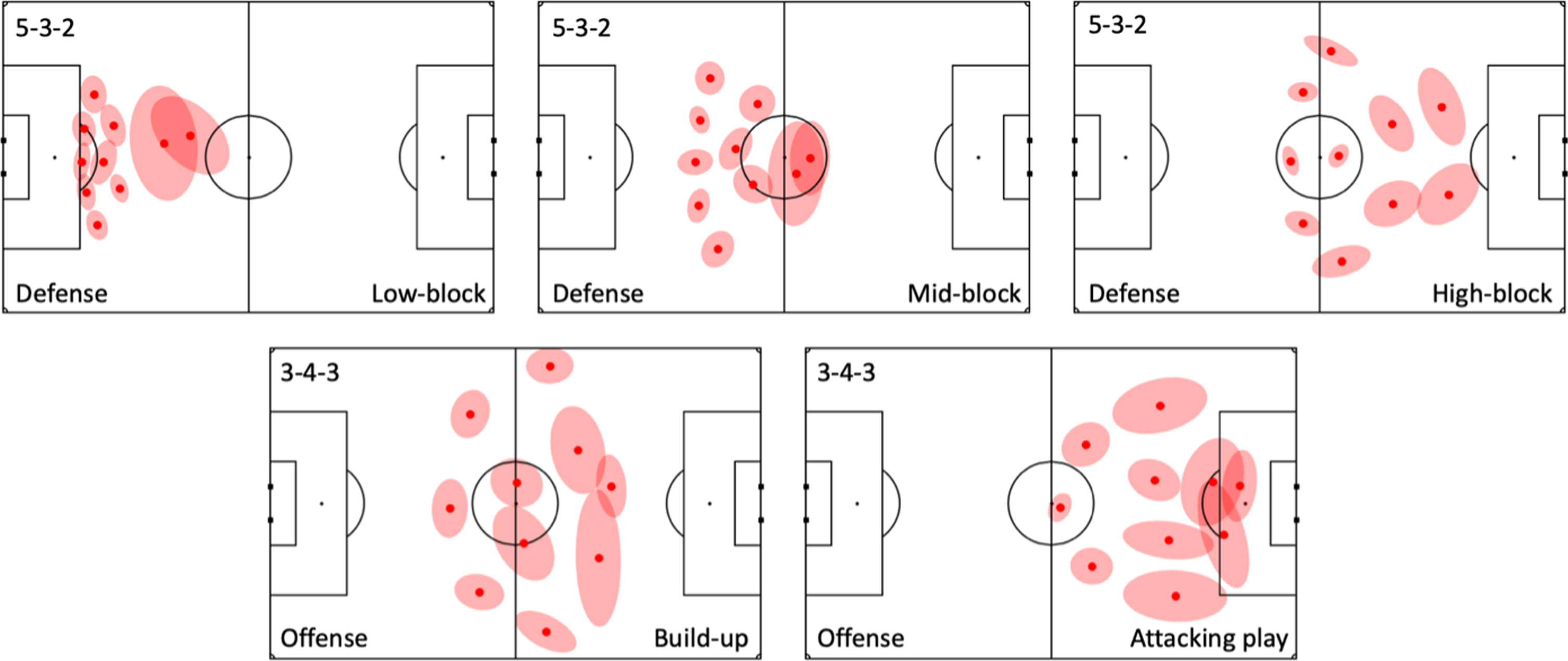
The figure clearly indicates that team formations do not only depend on which team is in possession of the ball, it is also heavily influenced by the tactical patterns teams are applying in different situations on the pitch, e.g. whether the team is currently building up in their own half or attacking in the last third of the pitch. Also, in defensive phases of play, Fig. 3 (lower row) shows significant differences depending on the teams defending strategy (high-/mid-/low-block).
4.2Measuring formation in distinct phases of play
A major objective of this work is to identify the distinct formations used by teams during different phases of play during their matches. We focus specifically on the three defensive phases (high-block, mid-block and low-block) and two offensive phases (build-up and attacking-play) shown in Fig. 1. Transitions and set-pieces are ignored: by definition, teams do not have a clear spatial structure during transitions, while positioning during set-pieces are extremely dependent on the position of the ball (Casal et al., 2015). Furthermore, as it takes some time for a team to change from one formation to another— for example, they cannot instantly shift from a high-block to a mid-block— we ignore the first three seconds of any continuous sequence of play that was classified to a single phase of play; if the duration of the entire sequence is less than three seconds, we discard it from our sample. In our case, the range of observations encompasses all frames classified to the same phase of play. At least 60 seconds of (aggregated) data are required to obtain a precise measure of a formation; if the total amount of time spent by a team in any given phase does not meet this criterium, we do not measure a formation for that phase.
Our method for measuring formations proceeds as follows: For each team, we aggregate together all the tracking data frames classified to a particular phase during the match and use them to measure the formation of the team in that phase. This is achieved using the methodology of Shaw et al. (2019), who introduced a geometric approach to measuring formations, calculating the vectors between each pair of teammates at a given instant during a match and averaging these over a range of observations (frames) to gain a clear measure of the team formation: each player’s position is calculated relative to the position of his nearest teammate. This process starts with the player in the centre of the team (specifically, the player with the lowest average distance to their third-nearest neighbor), stepping from player to player until the entire team formation is mapped out. This method is founded on the intuition that players orient themselves relative to their nearest teammates to retain the relative positioning required by the team’s formation.
A coach may, of course, make a major tactical change during a match, changing their team’s formations across all phases of play. To avoid mixing two different formation strategies within a match, we search for major tactical changes in formation by looking at each player’s average position relative to their teammates over a rolling time window. If the relative positions change for more than ten meters (based on a three-minute rolling average), we start a new set of formation observations; more details are given in Appendix B. At least one major change in formation of either team is found in 43% of matches— taking this factor into consideration presents a major improvement compared to prior work. In these games there are therefore two (or more) formation measures for each phase of play.
From the 2, 142 matches, we exclude 345 matches that did not end with 22 players on the pitch (e.g. due to injuries or expulsions) resulting in a final sample of 1, 803 matches. The final number of formation observations in each phase of play are given in Table 3. As discussed above, there was not always sufficient data to measure a formation in all phases of play during a match for both teams. Therefore, there are fewer observations in the least frequent phases, the low-block and high-block (furthermore, not all teams employ a high-block for tactical reasons). There are observations of the mid-block, build-up and attacking-play for almost all teams in every match in our sample (and, on occasion, more if a team made a major tactical change during the match).
Table 3
Included formation observations from seven years of the German Bundesliga (2013/2014 until 2018/2019)
| Tactical phase | Low-block | Mid-block | High-block | Build-up | Attacking-play |
| Formation observations | 1,212 | 5,200 | 638 | 4,867 | 3,164 |
4.3Formation classification
To study how a specific team plays over multiple matches, we must reduce the size of our formation dataset by identifying the unique formations within each phase of play over our entire sample of matches and classifying individual observations into these unique formations. The pioneering football coach, Marcelo Bielsa, has previously claimed that there are not more than ten formations7 in common use in professional football— our methods enable us to explore this claim directly. Classifying formations allows us to quantify the strengths and weaknesses of a given formation when pitted against another (Section 5.1), and study the preferred formations used by individual Bundesliga coaches (Section 5.2).
To identify unique formation types, we apply agglomerative hierarchical clustering to the formation observations within each phase of play, using the Wasserstein metric to quantify formation similarity and the Ward metric (Ward et al., 1963) as the linkage criterion, as described in Shaw et al. (2019). The square of the Wasserstein distance is calculated according to Olkin et al. (1982):
Figure 4 shows the unique formations identified in the most frequently observed defensive phases of play: the midfield-block. Results for all the most-frequently observed in-possession phases of play, build-up, are provided in Appendix C. All the formations shown were familiar to the match analysts that inspected them. Indeed, the analyst’s input was important in distinguishing the 4-2-3-1 formation from the 4-4-2: while the two appear similar in the figure, inspection of the individual observations that comprised each cluster indicated that the outside midfielders in the 4-2-3-1 (top-left plot) formed part of a triplet of attacking midfielders rather than two conventional wingers, as in the case of the 4-4-2 (top-center).
Fig. 4
Outcome of the clustering for mid-block including the number of observations (obs.) of our sample.
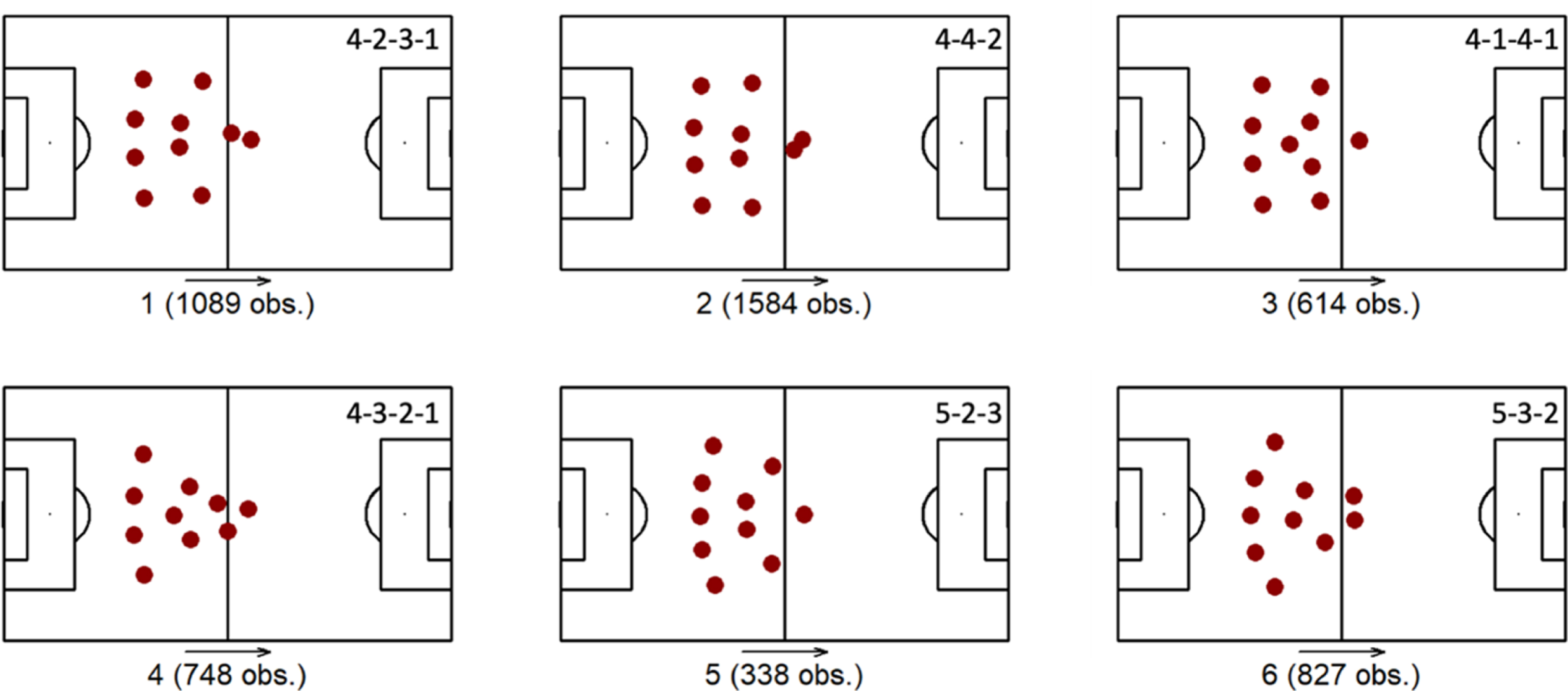
Formations #1–4 in Fig. 4 are all variants of a player configuration that uses four defenders as a foundation and are distinguished by differences in the structure of the midfield and attacking players. Formation # 3 sacrifices a forward for a central defensive midfielder, while formation # 4 is a narrow ‘Christmas tree’ formation8 (see also: Janetzko et al. (2015)) with three defensive midfielders, two attacking midfielders and a lone forward. The remaining two formations show variants of player configurations with five defensive players.
5Practical applications
The primary aim of this paper is to describe our methodology for automating the process of formation detection per phase of play. In this section we highlight two practical applications of our methods that are enabled by our approach.
5.1Formation versus formation
A very common question in tactical discussion is: what is the most effective way to counter a particular formation (Wilson, 2009)? This is a challenging question as it requires a large sample of formation observations as well as a contextualized formation detection per game-phase to attempt a quantitative answer. With over 13,081 formation observations measured over a sample of 1,803 Bundesliga games, we have a sufficient sample size to attempt a comparison of the relative performance of different formation options.
The most frequently observed offensive phase of play is the build-up; the most frequently observed formation in the build-up phase is the 2-4-3-1 (2 central defenders, 4 midfielders, 3 attacking midfielders and one forward), hereafter referred to as a ‘two-defender’ build-up. As the most frequently observed defensive phase of play is the mid-block, we attempt to quantify the performance of different mid-block formations in our data set when defending against a team using a two-defender build-up. Since goals are rare events in football9 and not all shots have an equal chance to score a goal, the concept of expected goals (xG) is often used as a more granular proxy for the offensive contribution of a team (Anzer et al., 2021a).10 XG values are only taken into consideration in periods of the match, where no formation change (see Appendix B) was detected. For such periods, xG values created from all phases of play were taken into consideration, since our experts claim that the formation in the basic phases of play (mid-block and build-up) has a latent influence on almost all situations.
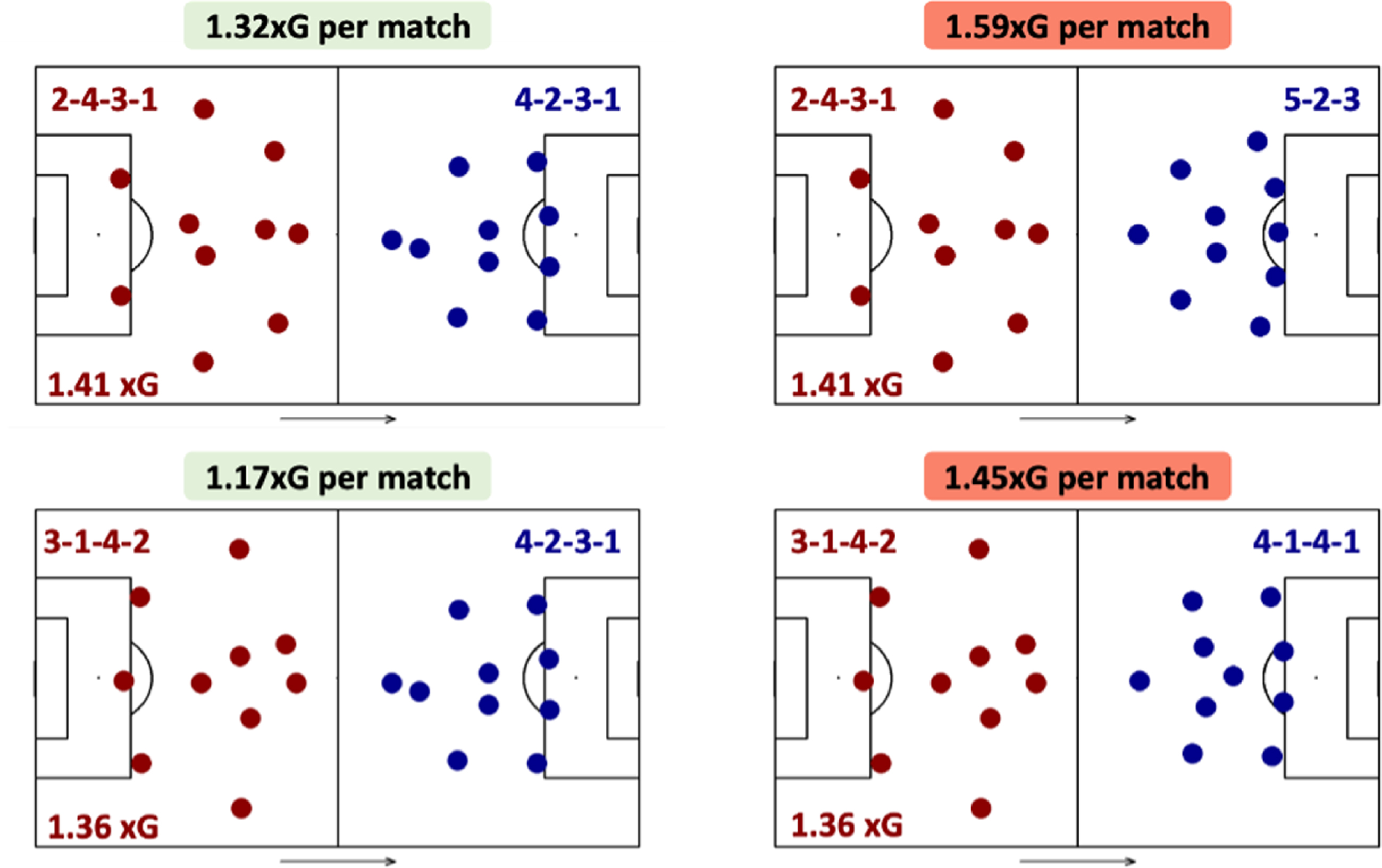
The top row of Fig. 5 shows the strongest and weakest mid-block options. A 4-2-3-1 concedes, on average, 1.32 (SE:±0.03; SD: ±0.81) xG11 per match against the two-defender build-up, while the 5-2-3 (a five-defender formation) concedes 1.59±0.06 xG per match. The unconditional scoring rate of the two-defender build-up formation is 1.41±0.02 xG per match; the 4-2-3-1 therefore appears to significantly reduce the attacking threat of the two-defender build-up, while the 5-2-3 is the least effective counter-formation. The difference between the two amounts to 0.27 xG per game, or nearly nine goals over a 34-game season.
An ongoing discussion in the football tactics community is whether a build-up with two or three central defenders is more effective (Wilson, 2009).12 In the lower row of Fig. 5 we repeat the exercise for the 3-1-4-2 build-up formation, which utilizes three, rather than two, players at the back. The base scoring rate of the three-defender build-up is 1.36±0.03 xG per game, slightly below the two-defender build-up formation. This drops to just 1.17±0.08 xG per game when facing a 4-2-3-1 mid-block formation (lower-left)— the most effective counter-formation— and increases to 1.45±0.08 xG per game against a 4-1-4-1 (lower-right, the weakest mid-block formation against a 3-1-4-2). The conclusion is that the three-defender build-up formation appears to be more easily countered than the two-defender formation while showing less of an up-side benefit against other formations. Building up with two defenders is significantly more popular amongst Bundesliga teams than building with three defenders; our results indicate that the latter does indeed appear to be a weaker option.
Fig. 5
Effectiveness of defensive formations (blue) against two (upper) and three (lower) player build-up (red).
Of course, even with a sample size of 1,803 matches, there are several potentially confounding factors, most notable if there is a preference for stronger (or weaker) teams to use a particular formation, although an initial inspection showed that every mid-block formation was used by at least 21 distinct teams once or more across the seven seasons. Future work (as described in the discussion) should investigate these confounding factors in significantly more detail.
5.2Scouting the tactical preferences of coaches
A major task that clubs must answer when seeking to fill a managerial vacancy is to ascertain the tactical preferences of the candidates and determine whether each represents continuity in the team’s existing tactical style or a significant departure. While some clubs may specifically seek a completely new style of play, there are considerable risks associated with this. Most notably, a new tactical system will require different players, creating turnover in the playing style as the new manager implements their preferred tactical systems and sells the players that they do not require. Our methods allow a characterization of the types of formations that coaches prefer to use, which is often a clear indication of their overall strategic preferences.
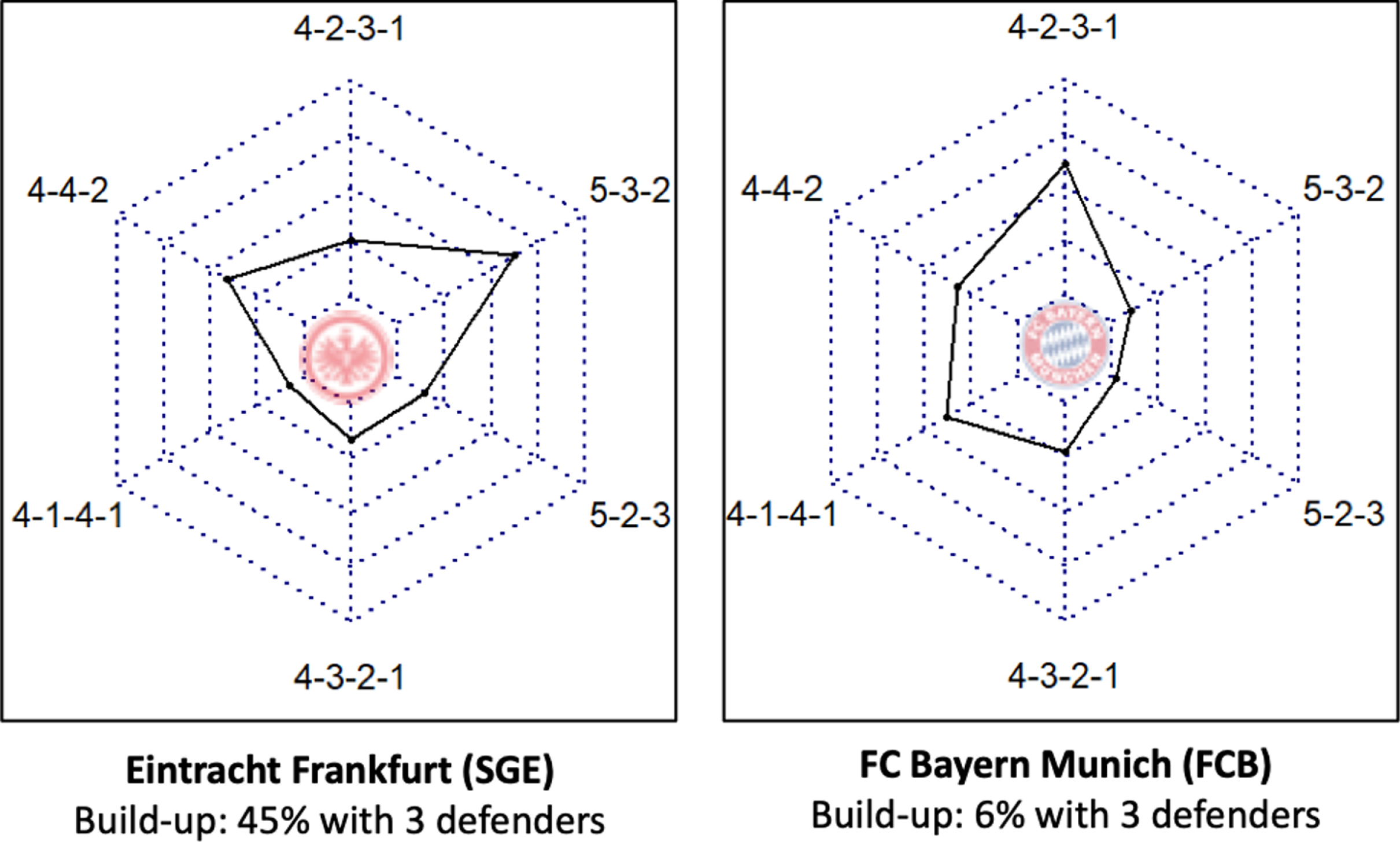
Individual teams demonstrate a preference for certain formations. Figure 6 compares the frequency with which a selection of Bundesliga clubs, have utilized different formation options in the mid-block phase (radar-charts). Whereas Eintracht Frankfurt tends to play in a modern 5-3-2 system, 3/22/2023Bayern Munich prefers the (somewhat similar) 4-2-3-1 or 4-1-4-1 systems. Another difference is that Bayern’s formation in the build-up phase is rather traditional, utilizing two central defenders, whereas Eintracht Frankfurt more regularly builds up with three central defenders, which aligns with their significantly preferred 5-3-2 mid-block formation.
Fig. 6
Formations used by selected German Bundesliga clubs in the mid-block phase.
This visualization shows how different teams’ preferences can be over a long period of seven seasons. These formation-profiles may often be determined by the key players of each team, some of whom may be particularly suited to one formation type. Bayern Munich’s success in the past few seasons has been greatly influenced by the central axis consisting of Jérôme Boateng, Robert Lewandowski and individually strong wingers like Frank Ribéry, Arjen Robben, Kingsley Coman or Serge Gnabry. Our match analysts agreed the formations most frequently utilized by Bayern’s coaches over the previous seven years— a 4-2-3-1 or a 4-1-4-1— are the most suitable formations for the players that were at the club.
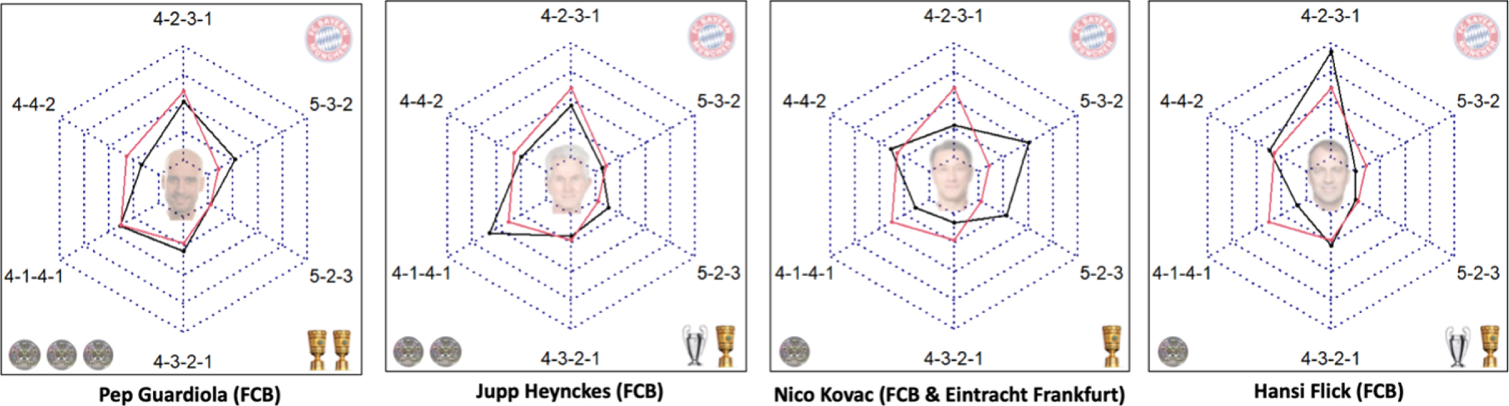
Figure 7 demonstrates the tactical preferences of four Bayern-coaches in the mid-block phase over this period. Guardiola, Heynckes and Flick all maintained a similar strategic approach, and all three had successful tenures. Only Niko Kovac is generally perceived to have been a failure. One reason, often referenced in the media, is that he was unwilling to part with the 5-3-2 build-up formation— with which he experienced success at his previous club, Eintracht Frankfurt— instead of adapting his style of play to exploit the full potential of the players at Bayern. The appointment of Niko Kovac did not represent continuity in Bayern’s playing style.
Fig. 7
FC Bayern Munich coaches by their formation (black) in comparison to the overall Bayern profile (red). The data from all coaches and FC Bayern are aggregated over the seasons 2013/2014 to 2019/2020. The trophies (Bundesliga Championship, DFB-Cup and UEFA Champions-League) that each coach earned at his time at FC Bayern are displayed.
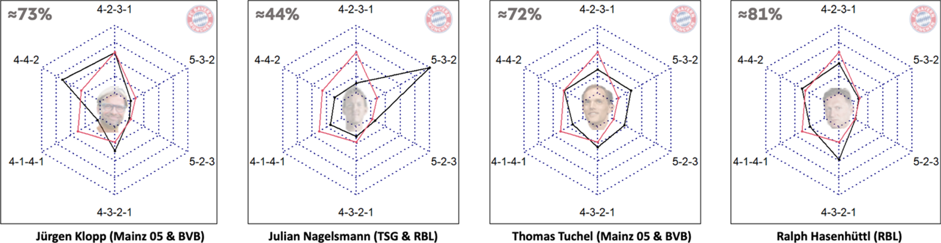
A valuable use-case of our methods is in the search for future managers with a similar playing style (at least in terms of formations) to the existing approach at the hiring club. Figure 8 shows a short-list of coaches that could be touted as potential successors of Hansi Flick— head coach at FC Bayern from 2019 until 2021. By comparing the coaches’ formation profiles (black)13 with that of FC Bayern (red) a similarity metric (top left in Fig. 8) can be calculated. Although Julian Nagelsmann (currently head coach at FC Bayern Munich) is often considered to be one of the biggest German coaching talents, his preferred formations diverge significantly from Bayern’s existing style, resulting in a similarity score of only 44%. Jürgen Klopp and Thomas Tuchel represent intermediate fits (72% and 73%), but Ralph Hasenhüttel, currently head coach of FC Southampton, is the best fit for FC Bayern in our managerial database, with a similarity score of 81%. Again, the choice of a coach relies on various factors, not solely on formations played in one or two phases of play (as displayed here). However, our approach provides evidence for one key component, which can drastically help club’s management to take informed decisions.
Fig. 8
Formation similarity. Who is the best fit for FC Bayern Munich? Top left the similarity of each coach compared to FC Bayern is displayed.
Note that similar to Section 5.1, a lot of confounding factors are neglected here. For example, the strength of a team, the personnel available to the coach, as well as opposing teams’ preferences influences a coaches playing style. Furthermore, the ability to adapt to a specific opponent is a central quality of a coach neglected by this analysis as well.
6Discussion
The availability of accurate and league-wide tracking data has motivated several research investigations into team formations, the basis of team-tactics in football. The main objective of this paper was to detect phases of play as a preliminary for contextualized formation analysis. Previous work has attempted to detect only single specific phases of play, such as counterattacking (Fassmeyer et al., 2021; Hobbs et al., 2018) or counterpressing (Bauer, 2021; Bauer et al., 2021). For the first time, we present a method for classifying games into five distinct phases of play. While the phases of plays used in our approach are well-established among football experts, their exact definitions may vary depending on a club’s playing philosophy. The definitions we used in the labeling process were consolidated among professional match analysts of German Bundesliga clubs. In future work, a proper qualitative study, that formalizes and extends the framework presented in Fig. 3 should be conducted in order to have a proper scientific baseline for further investigations on phases of play— a well-established theory in professional football. In this context, our work shows, that (a) phases of play can be defined and identified by experts with an appropriate accordance, and (b) that these phases of play influence the collective behavior of teams (i.e. their formations) significantly. However, we would like to highlight that since our phase-of play detection is based on training data from one specific season and only from the perspective of the home team, it ignores the evolution of the game throughout time and could be slightly biased since home and away teams can exhibit slightly different tendencies. Future work should therefore further evaluate whether the phase-of-play detection can be applied to multiple seasons and for both home and away teams with a similar accuracy.
We used this time-domain classification to measure team formations in distinct phases of play, achieving a spatial classification. Phases of play measurement and classification of formations represent a major step towards decrypting the complexities of strategy in football and provide a new insight into the tactical preferences of individual managers and coaches. While the methodology for the formation classification is mostly similar to the one introduced in Shaw et al. (2019), a crucial difference is not only that five different phases of play are considered separately, but also how closely subject experts were involved throughout the whole project. Selecting the final number of clusters purely on a statistical measure, would not lead to the same results as when taking expert-knowledge into consideration as well. This interplay between data-science and domain experts also turned out to be beneficial for the contextualization of the clusters, as well as for the identification of meaningful use-cases (see also Rein et al. (2016), Goes et al. (2020a), Andrienko et al. (2019), and Herold et al. (2019)). However, adding the formation per phase-of-play granularity also adds another layer of uncertainty, since we are building the clustering on top of a model with a known error rate (see Anzer et al. (2021a)). Especially, when we quote standard errors and standard deviations in Section 5.1, expected goal values may introduce an additional error source (see Anzer et al. (2021a)). Future work could use bootstrap methods to determine even more accurate estimations of the standard errors.
The benefit of our approach to practitioners is threefold: by automatically detecting phases of play of the next opponent over an arbitrary number of their previous games we save the match analysis departments significant amounts of time. An objective long-term analysis enables us to assess which formations are the most effective counter to a particular reference formation, drastically supporting a coaches decision-making process of how to approach the next opponent. Last but not least, we show a unique use-case for club decision-makers on how to quantify candidate coaches’ tactical style and identify those that represent continuity to the current playing style of the club.
Besides these applications, the full potential of this approach is yet to be unlocked. Future studies could analyse the interplay of different formations more thoroughly and control for confounding factors. On one hand, quantitative tendencies should always be evaluated by qualitative analysis, i.e. by analysing video footage of formation-pairings of interest to generate expert-based advantages and disadvantages when playing a specific formation (against another). On the other hand, the most critical confounding factor (the strength of a team playing a formation) should be modelled with a rating system of teams (e.g., Baysal et al. (2016)) and used to validate the hypothesis presented in Section 5.1. Additionally, when evaluating a coach’s tactical fingerprint, all phases of play as well as other factors could be taken into consideration.
Acknowledgements
This work would not have been possible without the perspective of professional match-analysts from world class teams who helped us to define relevant features and spend much time evaluating (intermediate) results. We would cordially like to thank Dr. Stephan Nopp and Christofer Clemens (head match-analysts of the German men’s national team), Jannis Scheibe (head match-analyst of the German U21 men’s national team), Leonard Höhn (head match-analyst of the German women’s national team) as well as Sebastian Geißler (former match-analyst of Borussia Mönchengladbach). Additionally, the authors would like to thank Dr. Hendrik Weber and Deutsche Fußball Liga (DFL) / Sportec Solutions GmbH for providing the positional and event data.
Appendix
A Detecting phases of play with a CNN
A schematic visualization of the CNN-architecture is displayed in Fig. 9.
Fig. 9
Schematic architecture of the CNN predicting the phases of play.
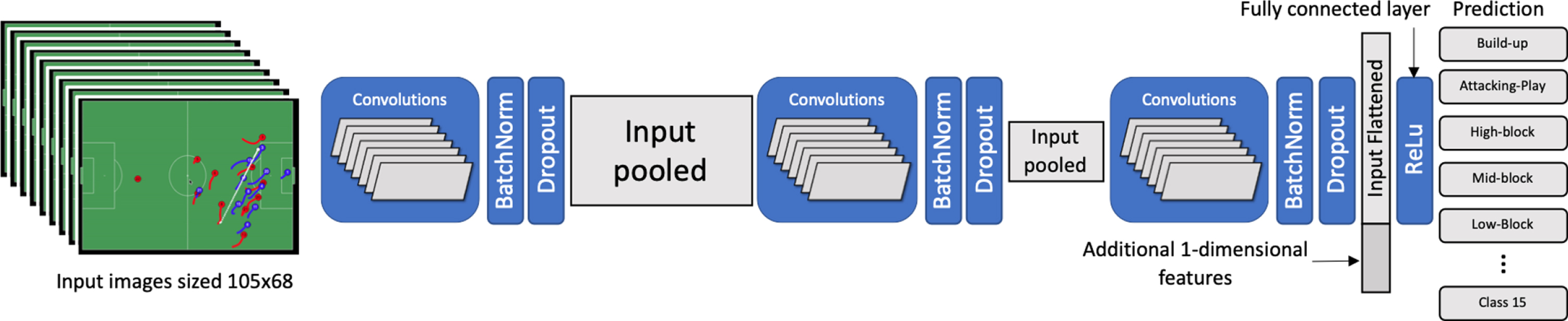
The input images are of size 105x68 pixels— corresponding to the typical dimensions of a football pitch in meters— and consist of up to nine layers (e.g. home-team positions, away-team positions, ball) containing information from a half-second period of the game. To feed time-related information to the CNN, player trajectories, weighted with a linearly decreasing function of time, were added to each image. To differentiate home team, away team and the ball, each information is imported as a separate layer. Additional layers contain smoothed speed values, which slightly improved the accuracy of our prediction. Finally, the CNN predicts one out of 15 possible phases of play1414 for each frame, although in this work only the phases shown in Fig. 1 in white boxes are taken into consideration. For each step of the 5-fold cross-validation we performed a Bayesian hyper-parameter optimization, whereby the final hyper-parameters represent the mean of all steps. The final model has a batch size of 32 and was trained over 10 epochs. The imbalanced dispersion of the phases of play (see Table 2) was addressed by resampling and weighted inputs for each batch. The best performing CNN yielding the highest F1-score on the test data consists of a base model with three convolutional layers, one fully connected layer and one concatenation with one-dimensional features. The additional features include for example a binary indicator whether the ball is in play, or the game is interrupted during the corresponding frame. Another feature, which is included in the positional data, is the information which team is currently in possession of the ball. This base model is applied at 13 consecutive time points (roughly half a second) and the outputs are combined using a 1-D convolution. It uses a drop-out of 50% and a ReLu-activation function. To avoid noisy outcomes in the framewise prediction, the outcome is smoothed afterwards by joining short sequences to its neighbouring sequences until each phase of play lasts at least one second.
B Detecting changes in formation
As tactical changes in the team formation may occur at any point in the game, we need to identify the moment when this may have happened. We use the following steps to approximate the moment when a change may have occurred. Our approach is player specific; for example, if two wingers switch sides at half time, we want to identify this as a change of formation. For simplicity we use the out of possession formations as a reference because they tend to be a bit more stable than while in possession. Therefore, we consider only the positional data of a team (excluding the goalkeeper), while the ball is in play and the opposing team is in ball possession.
We define the current formation position of a player as his average centered position, i.e. his mean average x and y coordinates relative to the team’s center (see also (Andrienko et al., 2017)), between the start of this formation (e.g. the beginning of the match, or the latest identified formation change) and the current time, t. His current formation position is then compared to his position during the last three minutes of eligible frames up to time t. If the Euclidean distance between any player’s current formation position and his three-minute rolling window position is greater than ten meters, we identify time t-minus-three minutes as the moment of a formation change and start to compute the current team formations starting at this time. Both thresholds were set by manually evaluating them on video footage with experts. Minor changes to these thresholds, do not strongly affect the presented results. Substituted players are compared to the position of the players they replaced. Using this algorithm over the past seven seasons of Bundesliga matches we identify on average 1.7 formation changes per match, which underpins the importance of this additional step to aggregating suitable sequences in our clustering step.
C Clustering for build-up
Figure 10 displays the clustering outcome of the second relevant phase–the build-up phase. As discussed in Section 1.1, a major decision that has to be made by a team is whether to build up with two central defenders (formations # 1, # 2, # 3, # 4) or with three central defenders (formations # 5 and # 6).15
Fig. 10
Outcome of the clustering for build-up including the number of observations (obs.) of our sample.
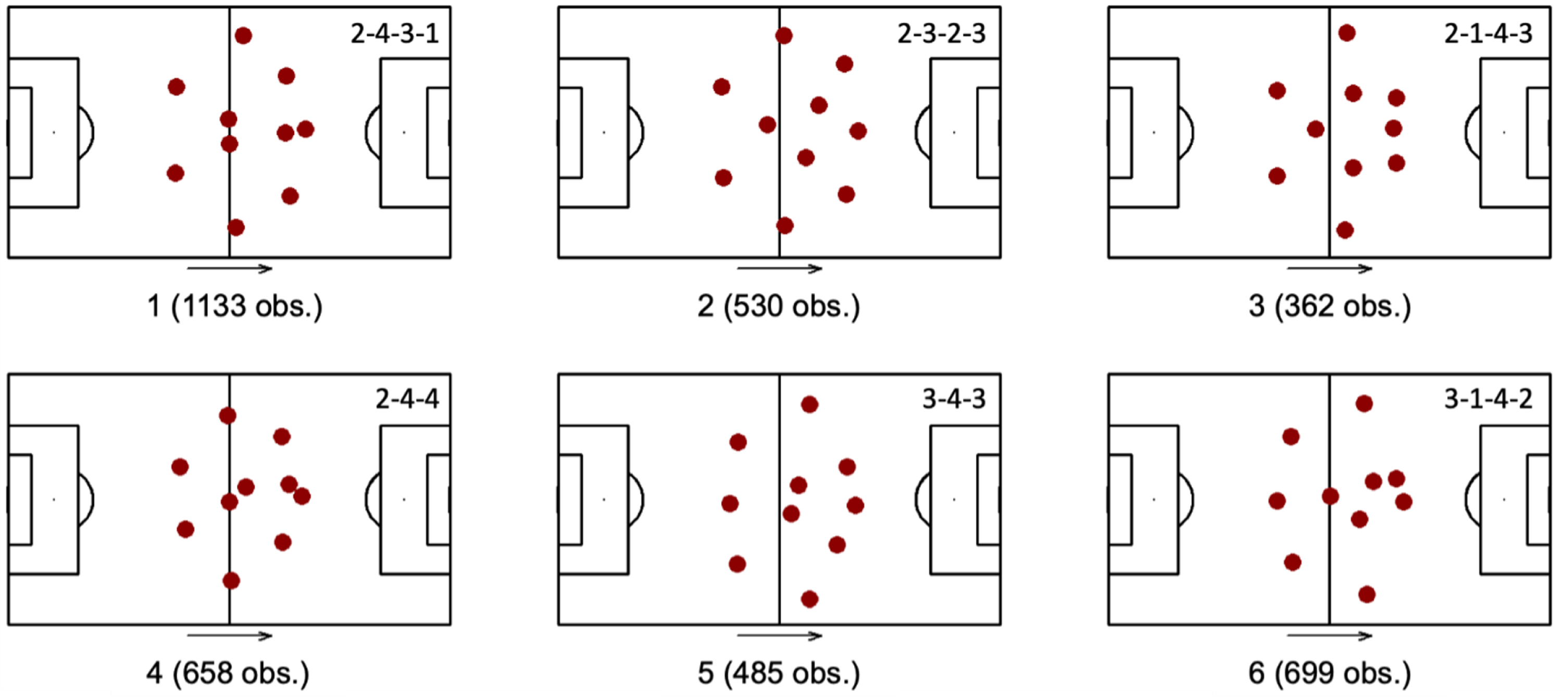
In Fig. 10, formation # 1 displays a 2-4-3-1 with two central defenders playing on the same line and the full-backs pushed into midfield. In formation # 4, one central midfielder clearly plays a more offensive role which allows the strikers not to participate in the build-up and rather plays a more offensive part, which was declared as a 2-4-4 by our experts. The formations shown in # 2 (2-3-2-3) and # 3 (2-1-4-3) also display similar patterns. The major difference is that the left and right striker tend to support the wing-back moving forward in # 2, whereas in formation # 3 all three strikers focus on playing in the center and leave the wings completely to the wing-backs. Formations # 5 (3-4-3) and # 6 (3-1-4-2) shows what our experts expected: building up with three central defenders provides a distinct flexibility during the build-up phase. A typical phenomenon when building up with three defenders is that the wing-backs have to conquer the wing-territories on their own, which should lead to a superiority in the center in both cases.
D Implementation details
While the newly available positional data allows for novel insights, the sheer size poses a significant computational challenge for non-IT-focused organisations such as football clubs or federations. All implementations were made in Python. We implemented the CNN (Section A) using Keras and Tensorflow and trained it on a local GPU-Cluster. Additionally, we used sklearn to perform the training test data split. In order to enable rapid feedback loops with match analysts, the tracking data is locally stored in Parquet files, compressing them from 500mb to 20mb per match. This step not only saves storage in the analytics environment but also enables us to read in an entire match in less than a second. For the computations necessary in this paper, the code is parallelized whenever possible to speed up the analysis even further.
Reference
1 | Alexander, J.P. Spencer, B. Sweeting, A.J. Mara, J.K. Robertson, S. (2019) , The influence of match phase and field position on collective team behaviour in Australian Rules football, Journal of Sports Sciences, 37: (15), 1699–1707.https://doi.org/10.1080/02640414.2019.1586077 (cit. on p. 3). |
2 | Andrienko, G. , Andrienko, N. , Anzer, G. , Bauer, P. , Budziak, G. , Fuchs, G. , Hecker, D. , Weber,, H. & Wrobel, S. , (2019) , Constructing Spaces and Times for Tactical Analysis in Football, IEEE Transactions on Visualization and Computer Graphics, 27: (4), 2280–2297.https://doi.org/10.1109/TVCG.2019.2952129 (cit. on pp. 2, 13). |
3 | Andrienko, G. , Andrienko, N. , Budziak, G. , Dykes, J. , Fuchs,, G. , vonLandesberger, T. & Weber, H. , (2017) , Visual analysis of pressure in football, , Data Mining and Knowledge Discovery, 31: (6), 1793–1839.https://doi.org/10.1007/s10618-017-0513-2 (cit. on pp. 7, 19). |
4 | António, D. , Pereira, P. , Vogais, F. , Doutora, P. , Volossovitch, A.G. , Filipe, R. , Duarte, L. , Do, C.E. & Pinto, C.C. , 2014, The emergence of team synchronization during the soccer match: understanding the influence of the level of opposition, game phase and field zone (cit. on p. 4). |
5 | Anzer, G. & Bauer, P. , Expected Passes—Determining the Difficulty of a Pass in Football (Soccer) Using Spatio- Temporal Data. Data Mining and Knowledge Discovery, Springer US. https://doi.org/10.1007/s10618-021-00810-3(cit. on p. 2). |
6 | Anzer, G. & Bauer, P. (2021) a, A Goal Scoring Probability Model based on Synchronized Positional and Event Data, , Frontiers in Sports and Active Learning (Special Issue: Using Artificial Intelligence to Enhance Sport Performance), 3: (0), 1–18.https://doi.org/10.3389/fspor.2021.624475 (cit. on pp. 2, 10, 13). |
7 | Anzer, G. Bauer, P. Brefeld, U. & Fassmeyer, D. (2022) b, Detection of tactical patterns using semi-supervised graph neural networks , MIT Sloan Sports Analytics Conference, Boston, USA (Winner research paper track 2022), 16: , 1–3.https://www.researchgate.net/publication/359079429_Detection_of_tactical_patterns_using_semi-supervised_graph_neural_networks (cit. on p. 1). |
8 | Anzer, G. Bauer,, P. & Brefeld, U. 2021b, The origins of goals in the German Bundesliga. Journal of Sport Science. https://doi.org/10.1080/02640414.2021.1943981 (cit. on p. 4). |
9 | Araújo, D. Couceiro, M. Seifert, L. Sarmento, H. & Davids, K. 2021, Artificial Intelligence in Sport Performance Analysis. https://doi.org/10.4324/9781003163589. (Cit. on p. 2). |
10 | Atmosukarto, I. Ghanem, B. Ahuj, A.S. Muthuswamy, K. & Ahuja, N. 2013, Automatic recognition of offensive team formation in american football plays,IEEE Computer Society Conference on Computer Vision and Pattern Recognition Workshops, 991-998. https://doi.org/10.1109/CVPRW.2013.144 (cit. on p. 2). |
11 | Balague, N. Torrents, C. Hristovski, R. Davids, K. & Araújo, D. (2013) , Overview of complex systems in sport , Journal of Systems Science and Complexity, 26: (1), 4–13.https://doi.org/10.1007/s11424-013-2285-0 (cit. on p. 1) . |
12 | Bauer, P. & Anzer, G. Data-driven detection of coun-terpressing in professional football—A supervised machine learning task based on synchronized positional and event data with expert-based feature extraction, Data Mining and Knowledge Discovery https://doi.org/10.1007/s10618-021-00763-7 (cit. on pp. 3, 5, 6, 12). |
13 | Bauer, P. Anzer, G. & Smith, J.W. 2022, Individual role classification for players defending corners in football (soccer), Journal of Quantitative Analysis in Sports https://doi.org/10.1515/jqas-2022-0003 (cit. on p. 1). |
14 | Bauer, P. 2021, Automated Detection of Complex Tactical Patterns in Football using Positional and Event Data—Using Machine Learning Techniques to Identify Tactical Behavior (Doctoral dissertation), Eberhard Karls University Tübingen. https://doi.org/10.15496/publikation-66042 (Cit. on pp. 1, 12). |
15 | Baysal, S. & Duygulu, P. (2016) , Overview of complex systems in sport, Journal of Systems Science and Complexity, 26: (7), 1350–1362.https://doi.org/10.1109/TCSVT.2015.2455713 (cit. on pp. 2, 13). |
16 | Beetz, M. , Hoyningen-Huene, N.V. , Bandouch, J. , Kirchlechner, B. , Gedikli, S. & Maldonado, A. (2006) , Camera-based observation of football games for analyz-ing multi-agent activities, Proceedings of the Interna-tional Conference on Autonomous Agents, 2006: , 42–49.https://doi.org/10.1145/1160633.1160638 (cit. on p. 1) |
17 | Brefeld, U. , Lasek, J. & Mair, S. (2019) , Probabilistic movement models and zones of control, Machine Learning, 108: (1), 127–147.https://doi.org/10.1007/s10994-018-5725-1 (cit. on p. 1) |
18 | Bianchi, F. , Facchinetti, T. & Zuccolotto, P. (2017) , Role revo- lution: Towards a new meaning of positions in basketball, Electronic Journal of Applied Statistical Analysis, 10: (3), 712–734.https://doi.org/10.1285/i20705948v10n3p712 (cit. on p. 2) |
19 | Bialkowski, A. , Lucey, P. , Carr, P. , Yue, Y. , Sridharan, S. & Matthews, I. 2014b, Large-Scale Analysis of Soccer Matches Using Spatiotemporal Tracking Data, IEEE International Conference on Data Mining, ICDM (Proceeding), (January), 725-730. https://doi.org/10.1109/ICDM.2014.133 (cit. on p. 2) |
20 | Bialkowski, A. , Lucey, P. , Carr, P. , Yue, Y. , Sridharan, S. & Matthews, I. 2015, Identifying team style in soccer using formations learned from spatiotemporal tracking data, IEEE International Conference on Data Mining Workshops, ICDMW, (January), 9-14. https://doi.org/10.1109/ICDMW.2014.167 (cit. on pp. 2, 7) |
21 | Bialkowski, A. , Lucey, P. , Carr, P. , Matthews, I. , Sridharan, S. & Fookes, C. (2016) , Discovering team structures in soccer from spatiotemporal data, IEEE Transactions on Knowledge and Data Engineering, 28: (10), 2596–2605.https://doi.org/10.1109/TKDE.2016.2581158 (cit. on pp. 2, 7) |
22 | Bialkowski, A. , Lucey, P. , Carr, P. , Yue, Y. & Matthews, I. 2014a, “Win at Home and Draw Away ”: Automatic Formation Analysis Highlighting the Differences in Home and Away Team Behaviors, MIT Sloan Sports Analytics Conference, (June 2016,http://www.sloansportsconference.com/wpcontent/uploads/2014/02/2014SSACWin-at-Home-Draw-Away.pdf (cit. on p. 7) |
23 | Borrie, A. , Jonsson, G.K. & Magnusson, M.S. (2002) , Temporal pattern analysis and its applicability in sport: An explanation and exemplar data, Journal of Sports Sciences, 20: (10), 845–852.https://doi.org/10.1080/026404102320675675 (cit. on p. 3) |
24 | Boon, B.H. & Sierksma, G. (2003) , Team formation: Matching quality supply and quality demand, Journal of Operational Research, 148: (2), 277–292.https://doi.org/10.1016/S0377-2217(02)00684-7 (cit. on p. 2) |
25 | Bourbousson, J. , Sève, C. & McGarry, T. (2010) , Space-time coordination dynamics in basketball: Part 2. the interaction between the two teams, Journal of Sports Sciences, 28: (3), 349–358.https://doi.org/10.1080/02640410903503640 (cit. on p. 7) |
26 | Bradley, P.S. , Carling, C. , Archer, D. , Roberts, J. , Dodds, A. , diMascio, M. , Paul, D. , Diaz, A.G. , Peart, D. & Krustrup, P. (2011) , The effect of playing formation on high-intensity running and technical profiles in English FA premier League soccer matches, Journal of Sports Sciences, 29: (8), 821–830.https://doi.org/10.1080/02640414.2011.561868 (cit. on p. 2) |
27 | Budak, G. , Kara, Iç, Y.T. & Kasımbeyli, R. (2019) , New mathematical models for team formation of sports clubs before the match, Central European Journal of Operations Research, 27: (1), 93–109.https://doi.org/10.1007/s10100-017-0491-x (cit. on p. 1) |
28 | Carling, C. (2011) , Influence of opposition team formation on physical and skill-related performance in a professional soccer team, European Journal of Sport Science, 11: (3), 155–164.https://doi.org/10.1080/17461391.2010.499972 (cit. on p. 2) |
29 | Casal, C.A. , Maneiro, R. , Ardá, T. , Losada, J.L. & Rial, A. (2015) , Analysis of corner kick success in elite football, International Journal of Performance Analysis in Sport, 15: (2), 430–451.https://doi.org/10.1080/24748668.2015.11868805 (cit. on p. 7) |
30 | Chen, , S. , Feng, Z. , Lu, Q. , Mahasseni, B. , Fiez, T. , Fern, A. & Todorovic, S. 2014, Play Type Recognition in Real-World Football Video, IEEE Winter Conference on Applications of Computer Vision, 652-659. https://doi.org/10.1109/WACV.2014.6836040 (cit. on p. 3) |
31 | Cintia, P. , Giannotti, F. , Pappalardo, L. , Pedreschi, D. & Malvaldi, M. The harsh rule of the goals: Data-driven performance indicators for football teams. In: Proceedings of the 2015 ieee international conference on data science and advanced analytics, dsaa 2015. Institute of Electrical; Electronics Engineers Inc., 2015, December. isbn: 9781467382731. https://doi.org/10.1109/DSAA.2015.7344823 (cit. on p. 2). |
32 | Danisik, N. , Lacko, P. & Farkas, M. Football match prediction using players attributes. In: Disa 2018 - ieee world symposium on digital intelligence for systems and machines, proceedings. Institute of Electrical; Electronics Engineers Inc., 2018, October, 201-206. isbn: 9781538651025. https://doi.org/10.1109/DISA.2018.8490613 (cit. on p. 2). |
33 | Decroos, T. , Van Haaren, J. & Davis, J. 2018, Automatic discovery of tactics in spatio-temporal soccer match data, Proceedings of the ACM SIGKDD International Confer- ence on Knowledge Discovery and Data Mining, 223-232. https://doi.org/10.1145/3219819.3219832 (cit. on pp. 2, 3, 5) |
34 | Decroos, T. , Van Haaren, J. , Bransen, L. & Davis, J. 2019, Actions speak louder than goals: Valuing player actions in soccer, Proceedings of the ACM SIGKDD International Conference on Knowledge Discovery and Data Mining, (1), 1851-1861. https://doi.org/10.1145/3292500.3330758 (cit. on p. 2) |
35 | Dick, U. & Brefeld, U. (2019) , Learning to Rate Player Positioning in Soccer, Big Data, 7: (1), 71–82.https://doi.org/10.1089/big.2018.0054 (cit. on p. 5) |
36 | Fassmeyer, D. , Anzer, G. , Bauer, P. & Brefeld, U. 2021, Toward Automatically Labeling Situations in Soccer, Frontiers Research Topic on Collective Behaviour in Team Sports (submitted 06/2021) (cit. on pp. 3, 5, 12). |
37 | Fernando, T. , Wei, X. , Fookes, C. , Sridharan, S. & Lucey, P. 2015, Discovering Methods of Scoring in Soccer Using Tracking Data, KDD Workshop on Large-Scale Sports Analytics, 1-4. https://large-scale-sportsanalytics.org/Large-Scale-Sports-Analytics/Submissions2015_files/paperID19-Tharindu.pdf (cit. on p. 3). |
38 | Fernandez, J. & Bornn, L. 2018,Wide Open Spaces : A statistical technique for measuring space creation in professional soccer, MIT Sloan Sports Analytics Conference, Boston (USA), 1-19 (cit. on p. 1). |
39 | Fujii, K. (2021) , Data-Driven Analysis for Understanding Team Sports Behaviors, Journal of Robotics and Mechatron- ics, 33: (3), 505–514.https://doi.org/10.20965/jrm.2021.p0505 (cit. on p. 1). |
40 | Goes, F.R. , Meerhoff,, L.A. , Bueno, M.J. , Rodrigues, D.M. , Moura, F.A. , Brink, M.S. , Elferink-Gemser, M.T. , Knobbe, A.J. , Cunha, S.A. Torres, R.S. & Lemmink, K.A. (2020) a, Unlocking the potential of big data to support tactical performance analysis in professional soccer: A systematic review, European Journal of Sport Science, 0: (0), 1–16.https://doi.org/10.1080/17461391.2020.1747552 (cit. on pp. 2, 13) |
41 | Goes, F.R. , Brink, M.S. , Elferink-Gemser, M. Kempe, M. & Lemmink, K.A. (2020) b, The tactics of successful attacks in professional association football—large-scale spatiotem-poral alanalysis of dynamic subgroups using position tracking data, Journal of Sports Sciences, 39: (5), 523–532.https://doi.org/10.1080/02640414.2020.1834689 (cit. on p. 1) |
42 | Goutte, C. & Gaussier, E. A Probabilistic Interpretation of Precision, Recall and F-Score, with Implication for Evaluation. In: Lecture notes in computer science. 3408. Springer Verlag, 2005, 345-359. https://link.springer.com/chapter/10.1007/978-3-540-31865-1_25 (cit. on p. 6) |
43 | Gréhaigne, J.F. Godbout, P. & Bouthier, D. (1999) , The foundations of tactics and strategy in team sports, Journal of Teaching in Physical Education, 18: (2), 159–174.https://doi.org/10.1123/jtpe.18.2.159 (cit. on p. 1) |
44 | Grunz, A. Memmert, D. & Perl, J. (2012) , Tactical pattern recognition in soccer games by means of special self-organizing maps, Human Movement Science, 31: (2), 334–343.https://doi.org/10.1016/j.humov.2011.02.008 (cit. on pp. 2, 3) |
45 | Gudmundsson, J. & Horton, M. (2017) a, Spatio-temporal analysis of team sports, ACM Computing Surveys, 50: (2), 1–34.https://doi.org/10.1145/3054132 (cit. on p. 1) |
46 | Gudmundsson, J. Laube, P. & Wolle, T. 2017b, Movement Patterns in Spatio-Temporal Data. Shekhar S., Xiong H., Zhou X. (eds) Encyclopedia of GIS. Springer, Cham. https://doi.org/10.1007/978-3-319-17885-1_823 (cit. on pp. 1, 2) |
47 | Haaren, J.V. , Zimmermann, A. , Renkens, J. , Broeck, G.V.D. , Beéck, T.O.D. Meert, W. & Davis, J. 2013, Machine Learning and Data Mining for Sports Analytics. https://doi.org/10.1007/978-3-030-64912-8. (Cit. on p. 2) |
48 | Herold, M. , Goes, F. , Nopp, S. , Bauer, P. Thompson, C. & Meyer, T. (2019) , Machine learning in men’s professional football: Current applications and future directions for improving attacking play, International Journal of Sports Science and Coaching, 14: (6), .https://doi.org/10.1177/1747954119879350 (cit. on pp. 2, 13) |
49 | Hochstedler, J. & Gagnon, P.T. 2017, American Football Route Identification Using Supervised Machine Learning, MIT Sloan Sports Analytics Conference, Boston (USA), 1-11 (cit. on pp. 2, 3). |
50 | Hobbs, J. , Power, P. , Sha, L. Ruiz, H. & Lucey, P. 2018, Quantifying the Value of Transitions in Soccer via Spatiotemporal Trajectory Clustering, MIT Sloan Sports Analytics Conference, Boston (USA), 1-11 (cit. on pp. 3, 5, 12). |
51 | Intille, S.S. & Bobick, A.F. 1999, Framework for recognizing multi-agent action from visual evidence, Proceedings of the National Conference on Artificial Intelligence, 518-525 (cit. on p. 2). |
52 | Janetzko, H. , Sacha, D. , Stein, M. , Schreck, T. Keim, D.A. & Deussen, O. Feature-driven visual analytics of soccer data. In: 2014 ieee conference on visual analytics science and technology, vast 2014 - proceedings. 2015. isbn: 9781479962273. https://doi.org/10.1109/VAST.2014.7042477 (cit. on p. 9). |
53 | Kempe, M. , Vogelbein, M. Memmert, D. & Nopp, S. (2012) , 2014, Possession vs. Direct Play: Evaluating Tactical Behavior in Elite Soccer, International Journal of Sports Science, 4: (6)A, 35–41.https://doi.org/10.5923/s.sports.201401.05 (cit. on pp. 3, 4) |
54 | Kempe, M. Grunz, A. & Memmert, D. (2015) , Detecting tactical patterns in basketball: Comparison of merge self-organising maps and dynamic controlled neural networks, European Journal of Sport Science, 15: (4), 249–255.https://doi.org/10.1080/17461391.2014.933882 (cit. on pp. 2, 3) |
55 | Kempe, M. 1955, The Hungarian method for the assignment problem, Naval Research Logistics (2), 83-97. https://doi.org/10.1002/nav.3800020109 (cit. on p. 8) |
56 | Li, R. & Chellappa, R. 2010, Group motion segmentation using a spatio-temporal driving force model, Proceedings of the IEEE Computer Society Conference on Computer Vision and Pattern Recognition, 2038-2045. https://doi.org/10.1109/CVPR.2010.5539880 (cit. on p. 3) |
57 | Link, D. & Hoernig, M. (2017) , Individual ball possession in soccer, PLoS ONE, 12: (7), 1–15.https://doi.org/10.1371/journal.pone.0179953 (cit. on p. 1) |
58 | Linke, D. Link, D. & Lames, M. (2018) , Validation of electronic performance and tracking systems EPTSunder field conditions, PLoS ONE, 13: (7), 1–20.https://doi.org/10.1371/journal.pone.0199519 (cit. on p. 3) |
59 | Linke, D. Link, D. & Lames, M. (2020) , Validation of electronic performance and tracking systems EPTSunder field conditions, PLoS ONE, 15: (3), 1–17.https://doi.org/10.1371/journal.pone.0230179 (cit. on p. 3) |
60 | Lucey, P. , Bialkowski, A. , Carr, P. , Morgan, S. Matthews, I. & Sheikh, Y. 2013, Representing and discovering adversarial team behaviors using player roles, Proceedings of the IEEE Computer Society Conference on Computer Vision and Pattern Recognition, 2706-2713. https://doi.org/10.1109/CVPR.2013.349 (cit. on p. 2) |
61 | Lucey, P. , Bialkowski, A. , Monfort, M. Carr, P. & Matthews, I. 2014, “Quality vs Quantity": Improved Shot Prediction in Soccer using Strategic Features from Spatiotemporal Data, Proc. 8th Annual MIT Sloan Sports Analytics Conference, 1- 9. http://www.sloansportsconference.com/?p=15790 (cit. on p. 3) |
62 | Montoliu, R. , Martín-Félez, R. Torres-Sospedra, J. & Martínez-Usó, A. (2015) , Team activity recognition in Association Football using a Bag-of-Words-based method, Human Movement Science, 41: , 165–178.https://doi.org/10.1016/j.humov.2015.03.007 (cit. on p. 3) |
63 | Müller-Budack, E. , Theiner, J. Rein, R. & Ewerth, R. 2019,“Does 4-4-2 exist?” –An analytics approach to understand and classify football team formations in single match situations, Proceedings Proceedings of the 2nd International Workshop on Multimedia Content Analysis in Sports (Nice, France), MMSports’(September), 25-33. https://doi.org/10.1145/3347318.3355527 (cit. on pp. 2, 3, 7) |
64 | Narizuka, T. & Yamazaki, Y. (2019) , Clustering algorithm for formations in football games, Scientific Reports, 9: (1), 1–8.https://doi.org/10.1038/s41598-019-48623-1 (cit. on p. 2) |
65 | Olkin, , I. & Pukelsheim, , F. (1982) , The distance between two random vectors with given dispersion matrices, Linear Algebra and Its Applications, 48: (100), 257–263.https://doi.org/10.1016/0024-3795(82)90112-4 (cit. on p. 8) |
66 | Pantzalis, V.C. & Tjortjis, C. Sports Analytics for Football League Table and Player Performance Prediction. In: 11th international conference on information, intelligence, systems and applications, iisa 2020. In-stitute of Electrical; Electronics Engineers Inc., 2020, July. isbn: 9780738123462. https://doi.org/10.1109/IISA50023.2020.9284352 (cit. on p. 2). |
67 | Pappalardo, L. , Cintia, P. , Rossi, A. , Massucco, E. , Ferragina, P. Pedreschi, D. & Giannotti, F. (2019) b, A public data set of spatio-temporal match events in soccer competitions, Scientific Data, 6: (1), 1–15.https://doi.org/10.1038/s41597-019-0247-7(cit. on p. 2) |
68 | Pappalardo, L. , Cintia, P. , Ferragina, P. , Massucco, E. Pedreschi, D. & Giannotti, F. (2019) a, PlayeRank: Data-driven performance evaluation and player ranking in soccer via a machine learning approach, ACM Transactions on Intelligent Systems and Technology, 10: (5). https://doi.org/10.1145/3343172 (cit. on p. 2) |
69 | Perse, M. , Kristan, M. Perš, J. & Kovacic, S. 2006, A Template Based Multi-Player Action Recognition of the Basketball Game, CVBASE’06 - Proceedings of ECCV Workshop on Computer Vision, 71-82 (cit. on p. 3). |
70 | Pettersen, S.A. , Johansen, D. , Johansen, H. , Berg-Johansen, V. , Gaddam, V.R. , Mortensen, A. , Langseth, R. , Griwodz, C. , Stensland, H.K. & Halvorsen, P. 2014, Soccer video and player position dataset, Proceedings of the 5th ACM Multimedia Systems Conference, MMSys 2014 (Singapore, March 2014), 18-23. https://doi.org/10.1145/2557642.2563677 (cit. on p. 3) |
71 | Pfeiffer, M. & Perl, J. (2015) , Analysis of tactical defensive behavior in team handball by means of artificial neural networks, IFAC-PapersOnLine, 28: (1).784–785 https://doi.org/10.1016/j.ifacol.2015.05.169 (cit. on p. 3) |
72 | Power, P. , Ruiz, H. , Wei, X. & Lucey, P. 2017, “Not all passes are created equal:” Objectively measuring the risk and reward of passes in soccer from tracking data. Proceedings of the ACM SIGKDD International Conference on Knowledge Discovery and Data Mining, Part F1296, 1605-1613. https://doi.org/10.1145/3097983.3098051 (cit. on p. 4) |
73 | Rein, R. & Memmert, D. (2016) , Big data and tactical analysis in elite soccer: future challenges and opportunities for sports science, SpringerPlus, 5: (1). https://doi.org/10.1186/s40064-016-3108-2 (cit. on pp. 1-3, 13) |
74 | Reep, C. & Benjamin, B. (1968) , Skill and Chance in Association Football Author, Journal of the Royal Statistical Society, 131: (4), 581–585.https://www.jstor.org/stable/2343726?seq=1 (cit. on p. 2) |
75 | Redwood-Brown, A. , Cranton, W. & Sunderland, C. (2012) , Validation of a real-time video analysis system for soccer, International Journal of Sports Medicine, 33: (8), 635–640.https://doi.org/10.1055/s-0032-1306326 (cit. on p. 3) |
76 | Ric, A. , Bradley, P. , Shaw, L. , Thies, H. , Sumpter, D. , López-felip, M.A. , Ade, J.D. , Dixon, J.A. , Evans, M. , Gómez-díaz, A. , Harrison, H.S. , Laws, A. , Petersen, M.N. , Seirul, P. , Robertson, S. , Pollard, R. , Bransen, L. , Kempe, M. & Bauer, P. 2021, Football Analytics 2021: The role of context in transferring analytics to the pitch, 158 (cit. on p. 2). |
77 | Sarmento, H. , Clemente, F.M. , Araújo, D. , Davids, K. , McRobert, A. & Figueiredo, A. (2018) , What Performance Analysts Need to Know About Research Trends in Association Football (2012–2016): A Systematic Review, Sports Medicine, 48: (4), 799–836.https://doi.org/10.1007/s40279-017-0836-6(cit. on p. 1) |
78 | Shaw, L. & Glickman, M. 2019, Dynamic analysis of team strategy in professional football, Barca sports analytics summit 1-13 (cit. on pp. 2, 3, 7, 8, 13). |
79 | Sampaio, , J. & Maçãs, V. (2012) , Measuring tactical behaviour in football, International Journal of Sports Medicine, 33: (5), 395–401.https://doi.org/10.1055/s-0031-1301320 (cit. on p. 2) |
80 | Siddiquie, B. , Yacoob, Y. & Davis, L.S. ( 2009) , Recognizing Plays in American Football Videos. Technical Report, University of Maryland, 1: (1), 1–8.http://www.researchgate.net/publication/228519111_Recognizing_Plays_in_AmericanFootball_Videos (cit. on p. 3) |
81 | Stein, M. , Janetzko, H. , Seebacher, D. , Jäger, A. , Nagel, M. , Hölsch, J. , Kosub, S. , Schreck, T. , Keim, D. & Grossniklaus, M. ( 2017) , How to Make Sense of Team Sport Data: From Acquisition to Data Modeling and Research Aspects, Data, 2: (1), 2.https://doi.org/10.3390/data2010002 (cit. on pp. 2, 3) |
82 | Stracuzzi, D.J. , Fern, A. , Ali, K. , Hess, R. , Pinto, J. , Li, N. , Tolga, K. & Shapiro, D. (2011) , An Application of Trans- fer to American Football : From Observation of Raw Video to Control in a Simulated Environment An Application of Transfer to American Football : From Observation of Raw Video to Control in a Simulated Environment, AI Magazine, 32: (2), .https://doi.org/10.1609/aimag.v32i2.2336 (cit. on p. 3) |
83 | Taberner, M. , O’Keefe, J. , Flower, D. , Phillips, J. , Close, G. , Cohen, D.D. , Richter, C. & Carling, C. (2020) , Interchangeability of position tracking technologies; can we merge the data?, Science and Medicine in Football, 4: (1), 76–81.https://doi.org/10.1080/24733938.2019.1634279 (cit. on p. 3) |
84 | Teoldo, I. , Manuel, J. & Greco, P.J. (2009) , Tactical Principles of Soccer Game: concepts and application. Motriz, Journal of Physical Education. UNESP, 15: (3), 657–668.https://doi.org/10.5016/2488 (cit. on p. 2) |
85 | Thinh, N.H. , Son, H.H. , Phuong Dzung, C.T. , Dzung, V.Q. & Ha, L.M. A video-based tracking system for football player analysis using Efficient Convolution Operators. In: International conference on advanced technologies for communications. 2019-Octob. IEEE Computer Society, 2019, October, 149-154. isbn: 9781728123929. https://doi.org/10.1109/ATC.2019.8924544 (cit. on p. 2). |
86 | Tierney, P.J. , Young, A. , Clarke, N.D. & Duncan, M.J. 2016, Match play demands of 11 versus 11 professional football using Global Positioning System tracking: Variations across common playing formations, Human Movement Science 49 (October), 1-8. https://doi.org/10.1016/j.humov.2016.05.007 (cit. on p. 2) |
87 | Vilar, L. , Araújo, D. , Davids, K. & Bar-Yam, Y. (2013) , Science of winning soccer: Emergent pattern-forming dynamics in association football, Journal of Systems Science and Complexity, 26: (1), 73–84.https://doi.org/10.1007/s11424-013-2286-z (cit. on p. 1) |
88 | Vilamitjana, J.J. , Heinze, G. , Verde, P. & Calleja-González, J. High-intensity activity according to playing position with different team formations in soccer. Acta Gymnica, 51 (March), 2-7. https://doi.org/10.5507/AG.2021.003 (cit. on p. 2) |
89 | Vogelbein, M. , Nopp, S. & Calleja-González, J. , (2014) , Defensive transition in soccer - are prompt possession regains a measure of success? A quantitative analysis of German Fußball-Bundesliga 2010/2011, Journal of Sports Sciences 32: (11), 1076–1083. https://doi.org/10.1080/02640414.2013.879671 (cit. on p. 3). |
90 | Wang, J. , Zhang, J. , (2015) , A win-win team formation problem based on the negotiation, Engineering Applications of Artificial Intelligence 44: , 137–152. https://doi.org/10.1016/j.engappai.2015.06.001 (cit. on pp. 1, 1386 2). |
91 | Wang, K.-C. , Zemel, R. , 2016, Classifying NBA Offensive Plays Using Neural Networks, MIT Sloan Sports Analytics Conference, 1-9 (cit. on p. 5). |
92 | Wang, Y , Wang, H. , Qiu, M. , Performance Analysis of Everton Football Club Based on Tracking Data. In: Proceedings of 2020 ieee international conference on power, intelligent computing and systems, icpics 2020. Institute of Electrical; Electronics Engineers Inc., 2020, July, 49-53. isbn: 9781728198736. https://doi.org/10.1109/ICPICS50287.2020.9202246(cit. on p. 2). |
93 | Ward, T. , Joe, H. , (1963) , Hierarchical 1399 Grouping to Optimize an Objective Function, Journal of the American Statistical Association 58: (301), 236–244 (cit. on p. 8). |
94 | Wei, X. , Sha, L. , Lucey, P. , Morgan, S. , Sridharan, S. , 2013, Large-scale analysis of formations in soccer. 2013 International Conference on Digital Image Computing: Techniques and Applications, DICTA 2013. https://doi.org/10.1109/DICTA.2013.6691503 (cit. on pp. 2, 7). |
95 | Wilson, J. , 2009, Inverting the pyramid, a history of football tactics. Orion. (Cit. on pp. 2, 9, 10). |
96 | Xu, H. , Prediction on Bundesliga Games Based on Decision Tree Algorithm. In: 2021 ieee 2nd international conference on big data, artificial intelligence and internet of things engineering (icbaie). IEEE, 2021, March, 234-238. isbn: 978-1-6654-1540-8. https://doi.org/10.1109/ICBAIE52039.2021.9389986(cit. on p. 2). |
97 | Yeh, R.A. , Schwing, A.G. , Huang, J. , Murphy, K. , 2019, Diverse generation for multi-agent sports games, Proceedings of the IEEE Computer Society Conference on Computer Vision and Pattern Recognition, 2019-June, 4605-4614. https://doi.org/10.1109/CVPR.2019.00474 (cit. on p. 1). |
98 | Zheng, S , Yue, Y. , Lucey, P. , 2016, Generating long-term trajectories using deep hierarchical networks, Advances in Neural Information Processing Systems, (Nips), 1551-1559 (cit. on p. 5). |
Notes
1 Link et al. (2017) showed that it is even less with large differences between playing positions: central forwards (0:49±0:43 min), central defenders (1:38±1:09 min), central midfielders (1:27±1:08 min) and, surprisingly, the longest for goalkeepers (1:38±0:58 min).
2 https://wheecorea.com/johan-cruyff-football-my-philosophy/25-johan-cruyff-quotes/, accessed 02/07/2021
3 An exemplary explanation of the definition can be found here: https://www.statsperform.com/resource/phases-of-play-an-introduction/.
4 https://chyronhego.com/wp-content/uploads/2019/01/TRACAB-PI-sheet.pdf (accessed 12/9/2022).
5 Other (non-scientific) open-source positional data sets can be accessed from Skillcorner (https://github.com/SkillCorner/opendata) or Metrica sports (https://github.com/metrica-sports/sample-data).
7 Marco Bielsa’s explanation of those ten formations can be found at https://www.youtube.com/watch?v=qXt3rKnfbz8 (accessed 12/06/2020).
8 The term Christmas tree formation— associated with a 4-3-2-1— has established in the football community (see https://thefalse9.com/2017/08/football-tactics-beginners-christmas-tree-formation.html, accessed 12/12/2020).
9 For the given data set of seven seasons of the German Bundesliga, 3.1 goals were scored in average per match.
10 The xG value of a shot denotes the a priori probability of a shot being converted to a goal, hence its value ranges from [0, 1]. The probability is estimated using both tracking and event data and applying a machine learning model, that was trained on more than 100.000 shots. A detailed description of the xG-model used can be found in Anzer et al. (2021a). Note that xG-values contain an error in itself, which influences all standard errors and standard deviations quoted in this section.
11 Errors quoted are the standard error on the mean.
12 An exemplary blog-article can be found here: https://thefalsefullback.de/2019/12/23/the-advantages-of-the-build-up-with-a-back-three/.
13 Note that only data from the respective coaches’ time in the German Bundesliga (2013/2014-2018/2019) are used for this analysis.
14 These 15 phases of play contain further splits for the transition phases (e.g. counterattacking, counterpressing) and set-pieces.
15 Note that for the formation versus formation contemplation in Section 5.1, the hierarchical clustering is further aggregated to n=2, so that only three-defender versus two defender build-up is compared.


