
Sports prediction and betting models in the machine learning age: The case of tennis
Abstract
Machine learning and its numerous variants have meanwhile become established tools in many areas of society. Several attempts have been made to apply machine learning to the prediction of the outcome of professional sports events and to exploit “inefficiencies” in the corresponding betting markets. On the example of tennis, this paper extends previous research by conducting one of the most extensive studies of its kind and applying a wide range of machine learning techniques to male and female professional singles matches. The paper shows that the average prediction accuracy cannot be increased to more than about 70%. Irrespective of the used model, most of the relevant information is embedded in the betting markets, and adding other match- and player-specific data does not lead to any significant improvement. Returns from applying predictions to the sports betting market are subject to high volatility and mainly negative over the longer term. This conclusion holds across most tested models, various money management strategies, and for backing the match favorites or outsiders. The use of model ensembles that combine the predictions from multiple approaches proves to be the most promising choice.
1Introduction
With the revival of long-known techniques in the context of exponentially more extensive calculation capabilities and data availability, “machine learning” is meanwhile part of many areas of science and daily life.1 Applications stretch from financial services to medicine and autonomously driving vehicles. The use in sports prediction and the associated betting markets has not received the same amount of attention so far. More traditional statistical approaches still dominate this field. Furthermore, one of the main focus areas has so far been the soccer market, with tennis – as one of the other major sports and betting marketplaces – receiving less attention.
Using a variety of models such as neural networks and random forests in conjunction with one of the most extensive datasets, this paper conducts a comprehensive study in the area of professional men’s and women’s tennis and as such addresses a critical research gap. It focuses on two fundamental questions. First, does machine learning outperform simple model-free forecasts that purely rely on the players’ official rankings or information implied from betting odds? In this context, also the informational content of various data features used in the models are examined. Second, are any of the techniques able to provide consistent positive returns for bettors?
All of the models are found to improve on the tennis ranking of both players as a sole indicator for the match prediction but are not able to outperform simple betting odds-implied forecasts. Differences in performance among the machine learning techniques are small. Odds from bookmakers are the most relevant data features for the models to predict the outcome of matches. Historical match and player data such as tournament series and round, age difference between opponents, or home advantage hardly add any additional explanatory power. Returns from model-based betting strategies are mainly negative over the long term and in nearly all cases exhibit high volatility. Ensembles of models that combine the signals of individual approaches are the most promising contenders for picking matches to bet on.
The paper is organized as follows. Section 2 offers an overview of previous work in the area of match prediction in professional tennis, with a particular focus on machine learning approaches. Section 3 describes the setup of the study and expands on the research objectives, data, and model features as well as the actual models and their calibration. Section 4 presents the results of the model predictions and also sheds light on the factors driving the performance. The application to the betting market covers the description of the decision rules, the money management strategies, and the resulting returns on investment. Section 5 concludes and provides an outlook for further research.
2Previous work
Sports events and the prediction of results through scientific analyses look back on a long history. The primary attention has been on soccer, with tennis being less in focus. As for tennis matches, Kovalchik (2016) groups prediction models into three broad categories: regression-based, point-based, and paired comparison. In addition, as part of several studies, predictions based on bookmaker odds are used for comparison (see, for example, Leitner et al. (2009)). Notably, the heterogeneous setup and data used in the various papers – in some cases in conjunction with only short forecasting horizons – demand cautiousness when comparing or even generalizing their findings.
Early examples of the first category of approaches, in which the probabilities for the match outcome are modeled directly, are the works by Clarke and Dyte (2000) and Klaasen and Magnus (2003). They calibrate logistic regression models to predict match outcomes based on ranking information. In Scheibehenne and Broeder (2007), the authors provide evidence that the mere recognition of players’ names by amateur players and laypeople outperforms predictions based on rankings and the seedings of experts. Online betting odds, however, perform even better.
Among the more comprehensive studies, Del Corral and Prieto-Rodriguez (2010) apply probit models calibrated using the players’ past performance, the players’ physical features, and match characteristics. Ranking information is found to be the most relevant for prediction accuracy. Individual men’s tournaments show significant differences, and being a former top-ten player is found relevant for women. Age differences have a significant effect for both men and women, albeit with different patterns. Ma et al. (2013) use logistic regression and calibrate it with variables reflecting player and match characteristics. They claim a pseudo-R2 of about 80% and correct identification of the winner in over 90% of the cases. In Lisi and Zanella (2017), the authors use a logistic regression model with features such as rankings, the players’ ages, the home advantage factor, and certain information derived from bookmaker odds. A betting strategy is said to result in a return of about 16%. Gu and Saaty (2019) combine data and “expert judgments” with the help of an analytical network process model. They report a prediction accuracy of about 85%, albeit for a very small sample of fewer than 100 matches.
Point-based models aim at estimating the probability of winning single points within a match and then derive expressions for the prediction of the overall match. For example, Barnett and Clarke (2005) use historical match data to predict single points and calculate the probability of the outcome of the entire match based on a Markov chain. Similarly, Knottenbelt et al. (2012) analyze a Markov model that yields a betting return of about 4%. Ingram (2019) makes a case for point-based models by using a Bayesian hierarchical approach for match prediction. Taking surface, tournament, and match date into account, he reports results that are comparable to those of the other model classes.
In paired comparison approaches, historical matches between players are aggregated to infer their respective strength ranking and predict future match outcomes. McHale and Morton (2011) advocate a probability model for paired comparisons, which they calibrate using tennis players’ past performance and the surface of the contest. When predicting future match results, they report superiority to logistic regression-based models, also in terms of achievable betting returns. Lyocsa and Vyrost (2018) use a paired-comparison model and investigate a range of betting rules based on odds and rankings. They cannot confirm achievable profitability as reported in McHale and Morton (2011) and instead conclude that there is at best only weak evidence for market inefficiency. Gorgi et al. (2019) propose a dynamic statistical model that accounts for time-varying player abilities across different court surface types. The authors claim that the model significantly outperforms those calibrated based on ranking information alone.
Kovalchik (2016) compares the three main types of models regarding their predictive performance for men’s singles matches. She confirms ranking information in regression models as best performing but ultimately not being able to beat bookmaker-implied forecasts.
The use of machine learning techniques is more of a novel area in sports prediction. In the world of tennis, only a few studies have been carried out so far. Table 1 summarizes the main ones, the models used, and their key findings. Despite a wide spectrum of approaches, data, calibrations, and evaluation metrics, overall, a prediction accuracy around the 70–75% mark is reported (with figures up to 99% being claimed). Most studies agree that models are generally not able to beat the predictions implied from bookmaker odds. Betting strategies with 3-4% of return on investment are presented (with claims reaching values of up to 80%). For some of the predictions but crucially the betting analyses, periods of usually not more than one year are used.
Table 1
Main studies using machine learning techniques for the prediction of professional tennis matches
| Author (s) | Modeling technique(s) and features | Data | Main finding(s) |
| Somboonphokkaphan et al. (2009) | Neural network (with a single hidden layer and up to 150 nodes) | Prediction for Grand Slam tournaments between 2003 and 2008, with varying model calibration windows between one and 22 years | Prediction accuracy of between 67% and 81% |
| Sipko (2015) | Logistic regression and neural network (with a single hidden layer and 100 neurons) | Prediction for ATP matches in 2013/14, with a model training period of about nine years | Neural network generating about 4% return on investment when applied to the betting market |
| Cornman et al. (2017) | Logistic regression, support vector machine (with a linear kernel), neural network (with a single hidden layer and 300 neurons), random forest | Prediction for matches of 2016/17 professional tennis season, with approximately 15 years of model training and validation data | •Prediction accuracy of approximately 70% •Betting strategy with an average yield of about 3% per match |
| De Araujo Fernandes (2017) | •Neural network (with a single hidden layer and four neurons) •Majority vote model, combining the neural network with two other approaches | Prediction for 2015 ATP and Grand Slam matches, with 2014 data used for model calibration | •Prediction accuracy of approximately 70% (ATP) and 75–80% (Grand Slam) |
| •Model prediction comparable to betting-implied forecasts and superior to using ranking information alone | |||
| Chavda et al. (2019) | Linear regression, decision tree, gradient boosting | Prediction for men’s US Open matches in 2016, with data between 2000 and 2015 used for model calibration | •Prediction accuracy of around 75% achieved with gradient boosting |
| •Models ultimately not able to beat the predictions implied from bookmaker odds | |||
| Gao and Kowalczyk (2019) | Logistic regression, support vector machine (with a radial basis function kernel), random forest | Prediction for ATP matches over the period 2000 to 2016 | •Prediction accuracy of about 83% (random forest), compared to 69% when using betting odds alone |
| •Ten-fold cross-validation only; no explicit prediction | |||
| Ghosh et al. (2019) | Decision tree, learning vector quantization, support vector machine (with a radial basis function kernel) | Prediction for men’s and women’s Grand Slam matches in 2013 | •Prediction accuracy of 92% to 99%, with decision trees showing the best performance |
| •Results holding for both explicit prediction and ten-fold cross-validation | |||
| Candila and Palazzo (2020) | Neural network (with a single hidden layer with up to 30 nodes) | Prediction for Grand Slam, Masters, and ATP Finals matches between 2013 and 2018, with a minimum of eight years of training period each | •Neural network outperforming competing methods (e.g., logistic regression) |
| •Betting strategies deliveringinvestment returns of up to 80% |
3Study design
3.1Research objectives
The aims of this study are twofold. First, it seeks to establish models and explanatory variables that determine the probability of the match favorite to win. The likelihood of the outsider (“longshot”) to win follows from that since the outcome in tennis is binary in nature.2 Representative models from various branches of the machine learning space are calibrated using match, player, and betting market data and put to the test. By using odds from the betting market as explanatory variables, it is also analyzed whether these alone – given their point-in-time character – encompass all relevant information. This hypothesis can be motivated by the “wisdom of the crowd” paradigm, i.e., the observation that the aggregation of estimates from a group of people is often more accurate than those of the individuals of that group.3 There is also evidence from a multitude of studies in this regard (see, for example, Kovalchik (2016)).4 A simple baseline prediction and a match forecast derived directly from bookmaker odds serve as challenger models.
Second, based on the prediction models, the profitability of strategies that place selected bets on fav-orite or longshot are evaluated. Additionally, model ensembles are used to test whether validating “signals” across multiple models bears value.
3.2Data and model features
The primary data for the study are records of the major men’s singles ATP (Association of Tennis Professionals) and women’s singles WTA (Women’s Tennis Association) matches,5 as well as those of the four Grand Slam tournaments, organized by the ITF (International Tennis Federation).6 Typical attributes found in the data are tournament series, location, court surface, match date and round, and the winner’s and loser’s ranking at the time of the match. In addition to the match data, player-specific information such as preferred hand, date of birth, and home country are obtained from the ATP and WTA websites, respectively. Besides the directly obtainable match and player attributes, certain additional features such as home and surface advantage and player “momentum” are derived as potentially useful explanatory variables.
In order to identify the players in a match unambiguously, their ATP or WTA rankings at the time of the tournament are used. This allows the determination of the favorite and the longshot.7 This distinction is not strictly necessary for the analysis since one could randomly assign the labels “Player A” and “Player B” and accordingly define the binary events of one of them winning.8 The pre-ordering of players by ranking, however, bears the advantage that a critical variable determining the probability of winning is already part of the setup and allows a straightforward definition of a meaningful baseline model – the favorite always wins. Subsequently, following this convention, any model provides the probability of the match favorite to win as output.9
The data is complemented by betting odds for both opponents of a particular match, as offered by the leading (UK) bookmakers. These quotes generally represent the most recent ones before the match. The study makes use of the average odds,10 typically derived from more than 20 bookmakers, as well as the maximum odds (i.e., the most favorable for a bettor).11 The odds are quoted as multiples of the betting amount, for example, 1.25. This means that for any 100 units bet, the bettor receives 125 back in case of a correct prediction. The study also makes use of the spread between the average and the best quotes in the market for both favorite and longshot. One can assume that the width of this spread holds additional information: for instance, the wider the spread, the less precise the market consensus.
Notably, bookmakers will not offer “fair” quotes that can be translated one-to-one into probabilities of events. First, there is a built-in margin – the overround – that constitutes the margin for the service. For example, with odds of 1.25 for the favorite and 3.30 for the longshot, in conjunction with a balanced demand for both events, the bookmaker is expected to make a profit of about 10% since 1/1.25 + 1/3.30≈1.10. Second, the bookmaker may deviate from the “true” probabilities when quoting odds in order to balance the demand, maximize betting volumes (profits), and exploit bettors’ biases.12
Therefore, betting odds are used directly as mo-del inputs, without postulating explicitly any adjust-ments.13 Sufficiently flexible models should be able to address, for example, any potential non-linear relationship between odds and probabilities for the match outcome. The only exception where an explicit transformation is required is creating a basic challenger model from betting odds. For that purpose, proportional normalization is applied, which translates the example odds above into implied probabilities of 72.5% and 27.5%, respectively.
While most of the data is available across all matches in the dataset, the need arises to handle missing information for certain features. For numerical variables (e.g., age of a player), the average across all available data is used; for categorical features (e.g., preferred hand), the most frequent value is taken. A summary of all model features and their definitions are provided in Table 2.
Table 2
Model features as explanatory variables for tennis match prediction
| ODDS.Avg.Favorite | Average bookmaker odds for the favorite |
| ODDS.Avg.Longshot | Average bookmaker odds for the longshot (outsider) |
| ODDS.SpreadMaxToAvg.Favorite | Spread between best and average odds for the favorite (positive by design) |
| ODDS.SpreadMaxToAvg.Longshot | Spread between best and average odds for the longshot (positive by design) |
| EXPL.Gender | Male or female tournament: with a joint dataset but evidence that the drivers for match outcomes are not the same for men and women (see, for example, Del Corral and Prieto-Rodriguez (2010)), any systematic differences can be captured with this indicator variable. |
| EXPL.Series | Tournament series (e.g., Grand Slam): more prestigious tournaments, also with higher prize money, tend to have a different composition of players in terms of strength and competitiveness. Furthermore, the liquidity and types of bettors in the market might be different between tournaments with and without a lot of media attention, which in turn can influence the odds-setting behavior of bookmakers (see, for example, Forrest and McHale (2007)). |
| EXPL.Round | Tournament round (e.g., semi-final): it is reasonable to assume that the incentives from substantially higher prize money in the later rounds – also consisting of the stronger players – have an influence (see, for instance, Gilsdorf and Sukhatme (2008)). |
| EXPL.RankDiffLog | Difference in ranking between longshot and favorite (positive by design): the rankings are expressed on a log-scale, as proposed, for example, in Klaassen and Magnus (2003) and Del Corral and Prieto-Rodriguez (2010) since the differences in the “quality” of the players are not linear. The ranking difference is more critical for the top-ranked field, and the log-transformation expresses this. The expected “loading” of the variable is positive: the higher the difference in ranking between two players, the higher the probability of the favorite to win. |
| EXPL.RankPointsDiffLog | Difference in ranking points between favorite and longshot (positive by design): expressed on a log-scale. Since it provides a more fine-grained view of the strength difference between the players than the rankings alone, it could contain additional information (see, for example, the discussion in Lisi and Zanella (2017)). |
| EXPL.DiffAge | Difference in age between favorite and longshot: the pattern is not so clear (see, for example, the discussion in Del Corral and Prieto-Rodriguez (2010)), but, as a tendency, one can expect the “loading” of this factor to be negative. If the favorite is (much) older than the longshot, his or her winning probability will – all else equal – be smaller. |
| EXPL.PreferredHand | Players’ preferred hand: there are four possible combinations (both right, both left, favorite right/longshot left, favorite left/longshot right). |
| EXPL.HomeAdvantage | Home advantage: if a tournament is held in a player’s home country, his or her home advantage is recognized. Among others, Koning (2011) reports a significant home advantage for men’s matches. In case only the favorite has home advantage, the variable is set to one. If only the longshot has home advantage, the indicator is set to minus one. In case both or neither of the two players have home advantage, the indicator equals zero. In this way, a single explanatory factor is obtained whose “loading” is assumed to be positive with regard to its contribution toward the favorite’s probability of winning the game. |
| EXPL.SurfaceAdvantage | Surface advantage: recognizing the influence of the match surface on players’ performance (see, for example, Martin and Prioux (2015)), their past games are analyzed, and the surface that they have been the most successful on (in relative terms) is declared as their preferred one (hard, clay, or grass). Then an equivalent indicator to the home advantage is formed, with values of plus one, zero, or minus one, depending on whether the match surface suits or does not suit the favorite and the longshot. Data availability permitting the “lookback period” is chosen as three years, as a compromise between a too short period (during which a significant preference is hard to establish) and an excessively long period (during which a player’s gameplay could have evolved). |
| EXPL.PlayerDuelsInThePast | Track record of the two opponents playing against each other: if the two have never played against each other in the past, the indicator is equal to zero. Otherwise, with
|
| EXPL.PlayerMomentum | Current form of a player: the player’s average ranking (on a log-scale) over the previous six months minus his or her current ranking. A positive (negative) value hence indicates that the player has been on a winning (losing) streak, and one can postulate that this “momentum” has an influence on the match at hand. Correspondingly, the expected “loading” of this factor is positive. |
The table provides an overview of the variables chosen to explain the probability of the favorite of a professional tennis match (according to ATP/WTA points) to win.
With the aggregated betting odds history only available from 2010 onward, the matched dataset – after some elementary corrections such as removing obvious erroneous entries – comprises approximately 39,000 match records, spanning 2010 through 2019. About 9,900 of those records stem from the Grand Slam series, and roughly 2/3 of the matches belong to the male tournament circuit.
3.3Models and their calibration
The following set of models is used:
1. Logistic Regression (LR).14 Stricto sensu, (binomial) LR is usually not considered part of the machine learning arsenal but an established standard when it comes to classification problems. With x as the vector of model features (e.g., the average betting odds for the favorite and the longshot) one seeks to predict y, representing whether the event in question (e.g., the favorite winning) occurs (y = 1) or not (y = 0), conditional on the model features:
(1)
The model fitting consists in determining the optimal vector θ including the constant θ0 and is accomplished by maximum likelihood. The model output are probabilities for the binary outcomes. In order to tune the model, a weighted L1 (Lasso) and L2 (Ridge) regularization is applied.15
2. Neural Network (NN).16 The input and output data are connected through a series of “layers.” In each layer, a linear transformation is applied to the data, followed by the application of a (non-linear) activation function. With a[0] as the input data, a[i] as the output of layer i and g as the activation function:
(2)
Layers other than the first and last are called “hidden” and can each consist of an arbitrary number of neurons. The calibration of the network consists in finding optimal weights W[i] and b[i] such that the output of the last layer fits the observations associated with the input data best.
As hyperparameters, the network structure – from a single hidden node to three fully connected hidden layers with fifty nodes each –, the penalties for L1 and L2 regularization, and the learning rate (that determines to what extent the weights are updated during the fitting process) are tuned.17
3. Random Forest (RF).18 It is a non-parametric model that generalizes a random tree model. The growing of each tree is achieved by repeatedly splitting the data, at each tree node, based on a randomly selected subset of features. The variable that maximizes information gain is chosen to be split on further. The ultimate model is built from averaging many trees trained like this. While the individual trees exhibit a low bias and high variance, the fact that they are mostly uncorrelated ensures that the final model averaging leads to a low variance.
For the purposes of tuning the RF model, its maximum tree depth and the number of randomly chosen features at each node are optimized.19
4. Gradient Boosting Machine (GBM).20 While a random forest relies on the idea of building an ensemble of models and uses averages of their predicted values, boosting methods are built on adding new models to the ensemble in a sequential way. In each iteration, a new “weak” learner model (with high bias and low variance) is trained with respect to the error of the ensemble so far. These new models are usually shallow trees or even just decision stumps (i.e., trees with only two leaves). Gradient boosting refers to a specific way of identifying the shortcomings of weak learners, by using gradients of the loss function.
Among the possible hyperparameters, the tree depth is found to be the one most useful to optimize.
5. Support Vector Machine (SVM).21 This method aims at separating the events into two categories (favorite winning or losing). With events represented as points in space, the SVM model uses hyperplanes that divide the categories in such a way that the largest distance to any point is achieved (“functional margin”). More formally, let x(i), i = 1, 2, . . . , N again be the vector of model features and y(i) be the binary outcome, coded as y(i)∈ { - 1 ;1 } to follow standard notation. With parameter vectors ω and b, the geometric margin for each observation is defined as
(3)
The model calibration entails solving the optimization problem
(4)
Regularization can be achieved by tuning the cost parameter C. With a problem not always lending itself to linear separability, a mapping of the data to a different space with the help of a kernel function K (xi,xi) is helpful. Here, linear, radial, and polynomial kernels are tested; their respective parameters serve as additional tuning parameters. Ultimately a linear one is chosen as the best performing.22
All data is standardized before entering the cali-brations. These are carried out with five-fold cross-validation to tune the hyperparameters.23
For comparison, two basic approaches are applied as challenger models:
• Baseline. The favorite (or longshot) always wins (i.e., with a probability of 100%).
• Bookmaker-implied. Using only the betting odds for both favorite and longshot without any model, probabilities for the match outcome are derived (see Section 3.2).
For the calibration and prediction process, it is essential to distinguish between a statistical model such as logistic regression and a decision rule that transforms the output of a model into an actual class prediction (e.g., win or loss). The latter requires a decision threshold (e.g., 50%) that assigns a given case to one of the groups. The aim of this study is to work with class probabilities wherever possible since these lend themselves well to applications in the betting market with its market-implied odds and associated probabilities. As far as required for the calibration and hyperparameter tuning, a model’s accuracy – the number of correct predictions (favorite wins or loses) as a proportion of all predictions – is used as the target for the optimization. This can imply decision thresholds different from 0.5 when assigning a match to one of the two classes. Other evaluation metrics whose values are threshold-dependent are calculated and reported as well (see Section 4.1.1).
As for the actual calibration and prediction, sliding windows are used. Starting with the period 2010 through 2012, three-year calibration windows are employed and then used to forecast the probabilities for the subsequent year – beginning with 2013. This choice represents a compromise between a too-long window (that ignores potential changes in player composition, gameplay, and betting markets over time) and a too-short one (that does not allow for statistically robust calibrations). The setup results in seven calibration (2010–2012 through 2016–2018) and prediction periods (2013 through 2019) in total.
4Results
4.1Model predictions
4.1.1Model fitting and prediction performance
The results of the model fitting (calibration) and prediction are summarized in Table 3. A variety of measures for binary classification problems is reported.24 With seven sets of calibrations and forecasts, the table provides the average figures in Panel A and B, respectively. About 12,000 matches are used for each calibration and 4,000 for each prediction. The best score for each performance measure across the models is highlighted.
Table 3
Performance metrics of selected tennis match prediction models
| Baseline | Bookmaker-implied | 1. Logistic Regression | 2. Neural Network | 3. Random Forest | 4. Gradient Boosting Machine | 5. Support Vector Machine | |
| A. Calibration | |||||||
| Number of matches | 11,792 | ||||||
| Log-loss | N/A | 0.568 | 0.567 | 0.568 | 0.558 | 0.565 | 0.572 |
| Brier | 0.336 | 0.194 | 0.193 | 0.193 | 0.189 | 0.192 | 0.195 |
| Calibration | 1.507 | 0.990 | 1.000 | 1.014 | 1.000 | 1.000 | 1.001 |
| Discrimination | 0.000 | 0.123 | 0.133 | 0.134 | 0.135 | 0.130 | 0.127 |
| AUC | N/A | 0.721 | 0.721 | 0.722 | 0.735 | 0.723 | 0.718 |
| Accuracy | 0.664 | 0.702 | 0.703 | 0.704 | 0.709 | 0.705 | 0.699 |
| Precision | 0.664 | 0.722 | 0.727 | 0.728 | 0.728 | 0.722 | 0.712 |
| Recall | 1.000 | 0.896 | 0.885 | 0.885 | 0.896 | 0.901 | 0.919 |
| Specificity | 0.000 | 0.318 | 0.344 | 0.348 | 0.339 | 0.316 | 0.266 |
| F1 | 0.798 | 0.800 | 0.798 | 0.799 | 0.803 | 0.802 | 0.802 |
| B. Prediction | |||||||
| Number of matches | 3,996 | ||||||
| Log-loss | N/A | 0.579 | 0.580 | 0.582 | 0.580 | 0.581 | 0.584 |
| Brier | 0.347 | 0.198 | 0.198 | 0.199 | 0.199 | 0.199 | 0.200 |
| Calibration | 1.532 | 0.993 | 1.005 | 1.017 | 1.003 | 1.004 | 0.993 |
| Discrimination | 0.000 | 0.116 | 0.124 | 0.121 | 0.116 | 0.117 | 0.121 |
| AUC | N/A | 0.712 | 0.710 | 0.709 | 0.710 | 0.708 | 0.707 |
| Accuracy | 0.653 | 0.690 | 0.690 | 0.689 | 0.690 | 0.691 | 0.689 |
| Precision | 0.653 | 0.710 | 0.715 | 0.714 | 0.712 | 0.708 | 0.703 |
| Recall | 1.000 | 0.888 | 0.875 | 0.875 | 0.883 | 0.895 | 0.908 |
| Specificity | 0.000 | 0.317 | 0.341 | 0.339 | 0.325 | 0.305 | 0.278 |
| F1 | 0.790 | 0.789 | 0.786 | 0.786 | 0.788 | 0.790 | 0.792 |
The table shows a selection of performance measures for both the model calibration and prediction of the outcome of professional tennis matches over the period 2010 through 2019. In total, 25,204 singles matches from the ATP schedule (men) and 13,755 matches from the WTA circuit (women) are used. The event in question is whether the favorite according to ATP/WTA points wins (“1”) or not (“0”). All models are calibrated over three-year windows and used for the subsequent year’s prediction. Hence, seven sets of calibrations (spanning 2010–2012 through 2016–2018) and predictions (2013 through 2019) are created; the table reports a range of performance metrics, averaged over all periods, in Panel A and B, respectively. The baseline model always predicts the favorite to win. The bookmaker-implied model combines the quoted odds for both the match favorite and longshot to infer the outcome probabilities directly, without an explicit model. The best score for each metric across the models is highlighted. AUC: Area Under the Receiver-Operating-Characteristic Curve.
The log-loss is defined as the negative average of the log-probabilities of the actual match outcomes. The closer to zero, the better the fit.25 All models show similar average performance figures for both calibration and prediction. This includes the bookmaker-implied metrics, indicating that there is hardly any advantage of the five models relative to this basic challenger approach. The same holds for the Brier (1950) score, which equates, broadly speaking, to the mean squared error of the prediction. If all actual wins were to be assigned a winning probability of 100% by the model, the Brier score would be zero, its best value. The calibration measure takes into account that a good forecast should show events – here, the favorite winning or losing – with the right frequency that matches the predicted probability.26 The aim is a ratio close to one. If it is smaller, the model tends to underestimate the wins of the favorite; if it is higher, it tends to overestimate them. For the baseline model, the calibration score is far larger than one since the model has a bias toward the favorite. All other models, including the bookmaker-implied one, show near-perfect calibration figures, which are also close to one at the prediction stage. The discrimination metric reflects a model’s ability to provide win forecasts for actual wins and loss forecasts for actual losses.27 The greater the discriminatory power of a model, the higher the value; zero indicates that the model lacks all discriminatory ability. This is, by construction, the case for the baseline.
The Area-Under-the-ROC-Curve (AUC), with values between 0.5 and 1.0, summarizes the performance of a classification model across different classification thresholds, which determine the assignment to one of the two possible groups (see the discussion in Section 3.3).28 All models lead to moderate AUC figures of around 0.7.
The accuracy of the models amounts to about 70% during the calibration and 69% during the prediction. The baseline model has an accuracy of about 66%, equal to the proportion of wins by the favorite across matches. The bookmaker-implied benchmark yet again shows a performance that is no different from that of the models. The precision (also: positive predictive value) is the proportion of “true positives” over all those classified by a model as positive. The closer the value to one, the higher the proportion of correctly predicted match wins by the favorite among all predicted wins. All models perform similarly in this regard with values of around 71-72%; for the baseline model, the precision is by design equal to the accuracy. The recall (also: sensitivity or true positive rate) is defined as the “true positives” in relation to the “true positives” plus “false negatives.” The closer the value to one, the lower the proportion of predicted losses by the favorite that were actually wins. A trivial way to achieve a perfect recall of 1.0 is to predict that the favorite wins all matches – as the baseline model does. Recall in isolation is therefore not a sufficient criterion. The other models show comparable figures across the peers. The specificity (also: true negative rate) provides the ratio between the “true negatives” and the “true negatives” plus “false positives.” The closer the value to one, the lower the proportion of predicted wins by the favorite that were in fact losses. All models exhibit rather low performance figures, which is a sign of predicting too many wins of the favorite. Finally, the F1 (also: traditional F-measure or balanced F-score) is the harmonic mean of precision and recall. The values across all models are very close to one another, indicating that the ability to balance the two performance measures is not very different across the model spectrum.29
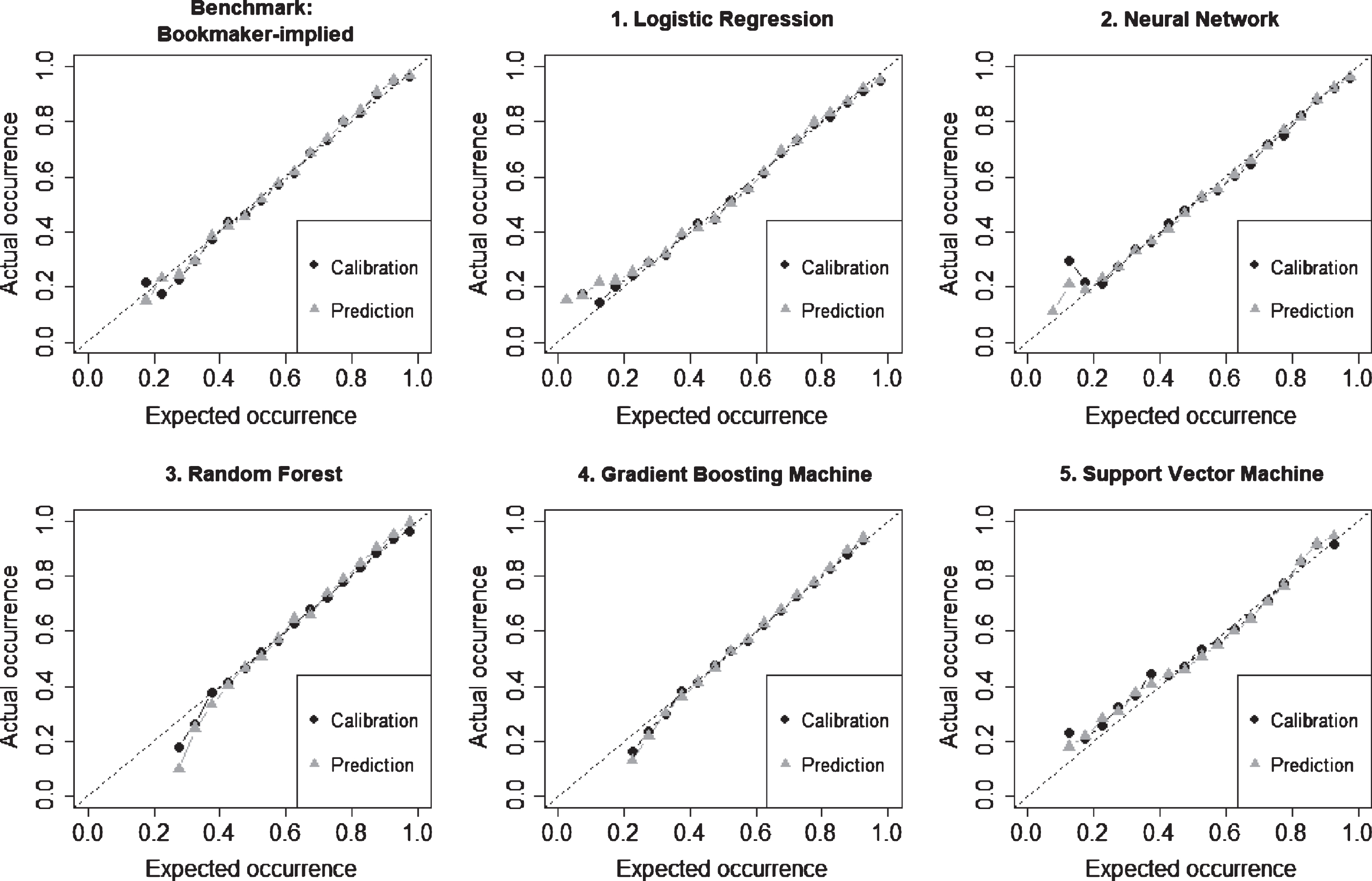
A convenient way of visualizing the models’ performance for both calibration and prediction sets is the use of bucketed frequencies of model predictions and actual outcomes. Figure 1 provides the results across the models, averaged over all periods. Deviations from the 45-degree line indicate that a model over- or underestimates the probability of the favorite to win. Most of the models show a good average performance, be it during calibration or during prediction. Slightly more pronounced differences appear in less populated buckets corresponding to small probabilities of the favorite to win (less than about 30%).
Fig. 1
Model performance across calibration and prediction datasets. This figure shows how well various models “fit” and predict the outcome of professional tennis matches. Each model – during calibration and prediction – determines the probability of the favorite to win a match. These probabilities are bucketed and compared to the actual match outcomes aggregated in the same way. Deviations from the 45-degree line indicate that a model over- or underestimates the probabilities for the favorite to win. Buckets with fewer than 25 observations are omitted. Given seven model calibrations (2010–2012 through 2016–2018) and predictions (2013 through 2019), the figures provide the averages over the datasets. The bookmaker-implied calibration and prediction serve as a benchmark: by combining the quoted odds for both the match favorite and longshot, one can infer the probabilities for the outcome.
4.1.2Feature importance
Table 4 provides an overview of the features (variables) and their significance across the models. Variable importance is expressed in percentage and sums to 100 for each case.30 The top-three variables for each of the datasets are highlighted. Not surprisingly, most models attribute a high relative importance to the bookmaker odds. This includes the spreads between average and maximum odds for both the favorite and the bookmaker.31 However, both the LR and NN model find attributes such as the players’ preferred hand and the series and round of the tournament as important for their respective calibrations.32
Table 4
Feature importance across selected tennis match prediction models
| 1. Logistic Regression | 2. Neural Network | 3. Random Forest | 4. Gradient Boosting Machine | 5. Support Vector Machine | |||||||||||
| Change in | Change in | Change in | Change in | Change in | |||||||||||
| Importance | Accuracy | AUC | Importance | Accuracy | AUC | Importance | Accuracy | AUC | Importance | Accuracy | AUC | Importance | Accuracy | AUC | |
| ODDS.Avg.Favorite | 9.6 | –4.2 | –4.3 | 8.9 | –5.6 | –8.2 | 34.1 | –2.0 | –2.2 | 28.9 | –2.5 | –2.2 | 34.3 | –17.0 | –27.9 |
| ODDS.Avg.Longshot | 23.6 | –3.6 | –13.9 | 5.2 | –0.4 | –2.5 | 24.5 | –1.7 | –2.1 | 26.5 | –1.0 | –2.0 | 25.8 | –3.8 | –5.8 |
| ODDS.SpreadMaxToAvg.Favorite | 0.7 | –0.1 | –0.1 | 1.9 | –0.5 | –0.5 | 14.0 | –0.5 | –0.6 | 14.1 | –0.9 | –0.5 | 5.8 | 0.0 | –0.1 |
| ODDS.SpreadMaxToAvg.Longshot | 6.9 | –0.7 | –0.6 | 4.0 | –0.1 | –0.8 | 15.3 | –0.2 | –0.8 | 15.2 | –0.6 | –1.1 | 6.9 | 0.1 | –0.1 |
| EXPL.DiffAge | 0.7 | –0.1 | 0.0 | 0.6 | 0.0 | 0.0 | 0.9 | –0.1 | –0.2 | 0.2 | 0.0 | 0.0 | 1.4 | 0.0 | –0.1 |
| EXPL.Gender | 2.6 | –0.1 | –0.1 | 6.6 | –0.3 | –0.2 | 0.1 | 0.0 | 0.0 | 0.0 | 0.0 | 0.0 | 0.5 | 0.0 | –0.1 |
| EXPL.HomeAdvantage | 6.3 | 0.0 | 0.0 | 7.3 | 0.0 | 0.0 | 0.2 | 0.0 | –0.1 | 0.0 | 0.0 | 0.0 | 1.2 | 0.0 | –0.1 |
| EXPL.PlayerDuelsInThePast | 0.4 | 0.0 | 0.0 | 0.5 | 0.0 | 0.0 | 0.3 | 0.0 | –0.1 | 0.1 | 0.0 | –0.1 | 0.5 | 0.0 | –0.1 |
| EXPL.PlayerMomentum | 0.5 | –0.1 | 0.0 | 1.3 | –0.1 | 0.0 | 0.9 | –0.1 | –0.3 | 0.4 | –0.1 | –0.1 | 1.5 | 0.0 | –0.1 |
| EXPL.PreferredHand | 21.4 | 0.0 | 0.0 | 14.0 | 0.0 | 0.0 | 0.2 | 0.0 | –0.1 | 0.0 | 0.0 | 0.0 | 6.9 | 0.0 | –0.1 |
| EXPL.RankDiffLog | 1.6 | –0.2 | –0.1 | 0.4 | –0.1 | –0.1 | 6.6 | –0.2 | –0.4 | 6.2 | –0.2 | –0.2 | 7.2 | 0.1 | –0.3 |
| EXPL.RankPointsDiffLog | 1.2 | 0.0 | 0.0 | 0.6 | 0.0 | 0.0 | 4.5 | –0.1 | –0.3 | 4.3 | –0.1 | 0.0 | 1.4 | 0.0 | 0.0 |
| EXPL.Round | 13.6 | –0.1 | –0.1 | 28.0 | –0.2 | –0.2 | 0.8 | –0.1 | –0.2 | 0.2 | 0.0 | 0.0 | 3.6 | 0.0 | –0.2 |
| EXPL.Series | 8.2 | –0.2 | –0.2 | 14.4 | –0.4 | –0.4 | 0.8 | –0.1 | –0.3 | 0.6 | 0.0 | –0.1 | 1.9 | 0.0 | –0.2 |
| EXPL.SurfaceAdvantage | 2.7 | 0.0 | –0.1 | 6.3 | –0.1 | –0.1 | 0.2 | 0.0 | –0.1 | 0.1 | 0.0 | 0.0 | 1.0 | 0.0 | –0.1 |
The table shows the feature importance when calibrating the outcome of professional tennis matches over the period 2010 through 2019. The “importance”of the explanatory variables is expressed in percent and adds up to 100 for each case. The top-three variables are highlighted in gray. Additionally, the absolute changes in “accuracy” and “AUC” (see Table 3) when dropping a specific variable from the model are reported; the largest differences are marked in bold. All figures are averaged over the calibration periods.
Given the easier interpretation, additionally, the change in accuracy and AUC (see Table 3) when removing certain features are shown,33 with the top-three each marked in bold. The dominant role of the bookmaker odds is confirmed, notably also for the LR and NN models since both show a high sensitivity here. Most of the other features play only a negligible role.
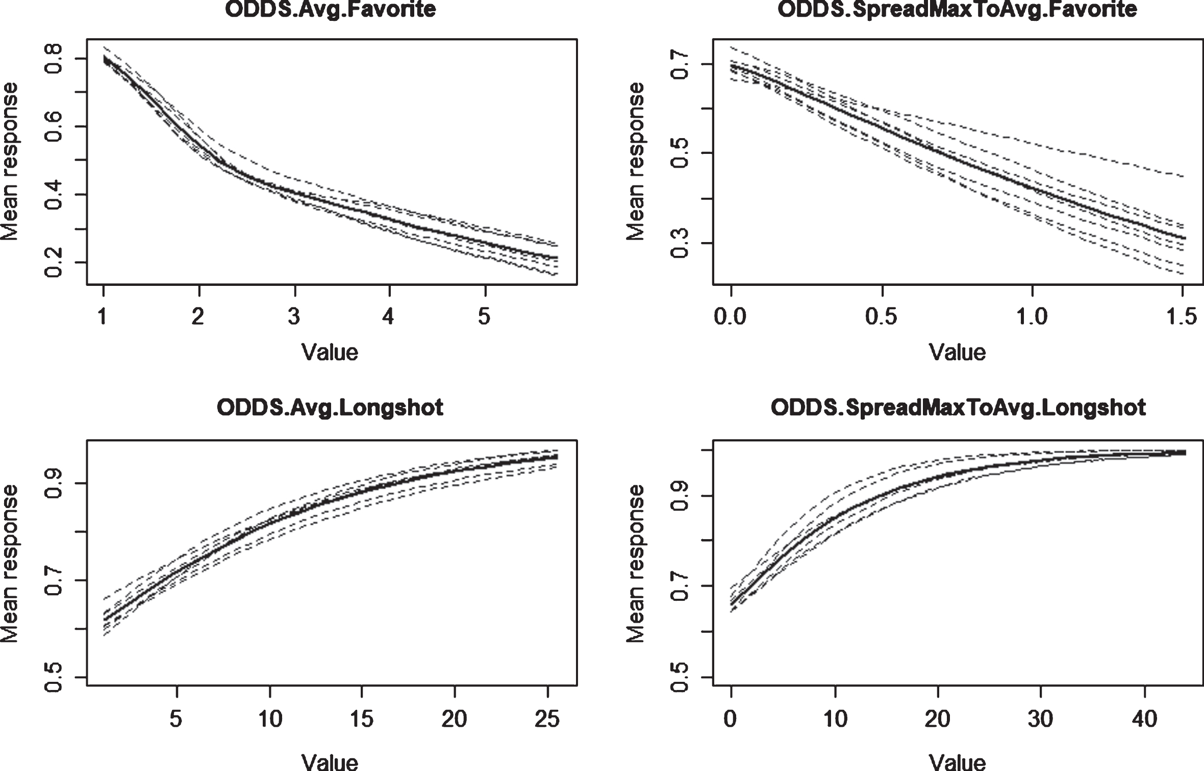
Partial dependence analysis is an intuitive tool to zoom deeper into the models’ driving factors.34 On the example of the NN model, Fig. 2 shows the marginal effects of the four variables reflecting the betting odds on the (mean) response, i.e., the probability of the match favorite to win. Besides the individual curves for each calibration period, their averages are shown as well. The graphs for ODDS.Avg.Favorite are downward-sloping with the value increasing, in line with the intuition that higher odds for the favorite go hand-in-hand with a lower probability of him or her winning a match. The spread between average and maximum odds for the favorite (ODDS.SpreadMaxToAvg.Favorite) exhibits a slig-htly less clear pattern but still confirms that the higher the spread, the lower the winning probability of the favorite, in line with expectation. For both the odds attached to the longshot (ODDS.Avg.Longshot) and the corresponding spread between average and maximum odds (ODDS.SpreadMaxToAvg.Longshot), the patterns are again as expected. The higher either of them, the higher the mean probability of the favorite to win –all else equal.
Fig. 2
Partial dependence plots on the example of the Neural Network model. This figure illustrates the marginal effects of the variables reflecting the betting odds on the example of the Neural Network model. The mean response reflects the probability of the match favorite to win. The results are shown for the seven calibration periods (2010–2012 through 2016–2018), together with their respective averages.
4.2Betting strategies
4.2.1Decision rules
In order to apply the calibrated models to actual betting strategies, the model-implied odds for the favorite to win (lose) are used to decide whether to place a bet or not. The market consensus in the form of the (a) average odds or (b) maximum odds thereby serves as a reference.35 For example, if the model implies a probability of the favorite to win of 80%, bookmaker odds of more than 1/0.8 = 1.25 would be considered worth betting on.
As a key additional feature, model ensembles are created. These combine the “signal” from the five models and only recommend a bet if at least N of them agree (N = 2, 3, ..., 5) The technique is well-established and especially useful if the individual models process the input data in different ways; the agreement of several of them is a strong sign that the inherent indication is valid. In case a model ensemble produces a betting proposition, the averages of the model-implied probabilities and betting odds of the individual approaches are used.
Working with ensembles also renders the derivation of additional “rules” such as a minimum margin (model-implied odd vs. betting odd) less relevant. The combination of predictions reduces the risk of being too sensitive and thereby placing bets too easily with only very small margins or poor risk-reward ratios. In the following, purely as a “numerical” safety margin, the minimum advantage of the odds is required to be 0.01 in absolute terms and 1% in relative terms.
The actual strategies are each carried for all combinations of model, odds type (average or maximum), betting side (favorite or longshot), and betting size (see Section 4.2.2).
4.2.2Betting sizes
In case a bet is placed on a particular match outcome, five different strategies for the betting sizes are evaluated:36
I. A fixed amount per bet
II. A fixed proportion of the current bankroll
III. Fixed expected return: an amount proportional to the inverse of the betting odd (example: for an odd of 1.6, one would place a bet of 1/1.6 = 0.625); this leads to lower (higher) bets if the risk is higher (lower) and ensures that the potential winnings, in absolute terms, are the same across bets
IV. A fraction of the current bankroll according to the Kelly (1956) criterion; it is based on the principle of maximizing the expected value of the (logarithm) of the bettor’s wealth and supposed to almost surely lead to higher wealth than any other strategy in the long run37
V. Variance optimization: as suggested in Rue and Salvesen (2000), the betting amount is chosen so that the difference between the expected gain and the variance of that gain is minimized; the optimal amount is thereby proportional to the odds and the probability of losing the bet
An implicit condition for Strategies I, III, and V with absolute betting amounts is that the bankroll is sufficient to sustain all potential losses. The fixed amount per bet, required for Strategy I, is set to one. The starting bankroll, explicitly needed for Strategies II and IV, is assumed as 1,000 and replenished every year. The proportion of the bankroll to bet as per Strategy II is set to 1% (i.e., starting with 10). In order to avoid an early quasi-bankruptcy, the Kelly proportion according to Strategy IV is capped at 1% of the prevailing bankroll. Note that for the trivial baseline model, this proportion would always be 100% (since the assumed outcome of the bet is certain), and the cap of 1% of the bankroll is hence always active. The outcome is thus the same for Strategies II and IV. The variance-optimized Strategy V demands model probabilities of less than one and is therefore ill-defined for the baseline model.
4.2.3Return on investment
The seven sets of predictions spanning 2013 through 2019 are aggregated and reported in Tables 5a and 5b when using average and most favorable bookmaker quotes, respectively. Results are shown for bets on the matches’ favorites as well as on the longshots. The summary comprises the number of matches, the proportion of matches that bets are placed on, which percentage of these are won as well as resulting returns. These are defined as profits and losses (P&L) divided by the wagered amounts over a given period. The criteria for comparing the strategies are both the “raw” and “risk-adjusted” returns, with the latter as the raw figure divided by the corresponding volatility.38
Table 5a
Results from betting strategies based on selected tennis match prediction models – using average bookmaker quotes
| Returns (%) | ||||||||||||
| Bets placed (%) | Bets won (%) | I. Fixed amount | II. Fixed proportion | III. Fixed expected return | IV. Kelly criterion | V. Variance-optimized | ||||||
| Raw | Risk-adj. | Raw | Risk-adj. | Raw | Risk-adj. | Raw | Risk-adj. | Raw | Risk-adj. | |||
| A. Betting on favorite | ||||||||||||
| 0. Baseline | 100.0 | 65.3 | –5.2 | –0.07 | –5.1 | –0.07 | –4.7 | –0.06 | –5.1 | –0.07 | – | – |
| 1. Logistic Regression | 7.3 | 59.6 | –1.3 | –0.02 | –1.4 | –0.02 | –1.8 | –0.02 | –1.4 | –0.02 | –0.3 | 0.00 |
| 2. Neural Network | 22.0 | 57.9 | –5.4 | –0.06 | –5.7 | –0.07 | –4.8 | –0.06 | –5.7 | –0.07 | –3.2 | –0.04 |
| 3. Random Forest | 7.1 | 41.9 | –5.2 | –0.04 | –5.4 | –0.05 | –3.3 | –0.03 | –5.2 | –0.04 | –2.4 | –0.02 |
| 4. Gradient Boosting M. | 11.4 | 54.3 | –3.8 | –0.04 | –3.9 | –0.04 | –3.5 | –0.04 | –3.8 | –0.04 | –4.0 | –0.04 |
| 5. Support Vector M. | 15.5 | 65.2 | –3.8 | –0.05 | –4.1 | –0.06 | –3.7 | –0.05 | –4.1 | –0.06 | –3.6 | –0.05 |
| 6. Ensemble (N = 2) | 15.8 | 54.1 | –3.9 | –0.04 | –4.1 | –0.04 | –3.7 | –0.04 | –4.1 | –0.04 | –3.5 | –0.04 |
| 7. Ensemble (N = 3) | 4.6 | 51.9 | –1.1 | –0.01 | –1.3 | –0.01 | –1.3 | –0.01 | –1.3 | –0.01 | –2.9 | –0.03 |
| 8. Ensemble (N = 4) | 0.8 | 57.2 | 7.6 | 0.08 | 7.6 | 0.08 | 8.6 | 0.09 | 7.7 | 0.08 | 9.8 | 0.10 |
| 9. Ensemble (N = 5) | 0.1 | 41.7 | –26.8 | –0.30 | –23.9 | –0.27 | –23.0 | –0.26 | –23.8 | –0.27 | –19.0 | –0.21 |
| B. Betting on longshot | ||||||||||||
| 0. Baseline | 100.0 | 34.7 | –9.5 | –0.06 | –10.9 | –0.07 | –6.6 | –0.04 | –10.9 | –0.07 | – | – |
| 1. Logistic Regression | 10.8 | 40.1 | –4.1 | –0.03 | –3.2 | –0.02 | –2.0 | –0.02 | –3.4 | –0.03 | –1.8 | –0.01 |
| 2. Neural Network | 12.4 | 41.3 | –4.6 | –0.04 | –3.5 | –0.03 | –3.3 | –0.03 | –3.1 | –0.03 | –3.7 | –0.03 |
| 3. Random Forest | 10.5 | 32.2 | –10.7 | –0.06 | –10.6 | –0.06 | –5.9 | –0.04 | –10.0 | –0.06 | –4.8 | –0.03 |
| 4. Gradient Boosting M. | 14.6 | 29.9 | –13.8 | –0.08 | –14.0 | –0.08 | –9.4 | –0.05 | –12.9 | –0.07 | –7.5 | –0.04 |
| 5. Support Vector M. | 28.3 | 33.4 | –11.7 | –0.07 | –11.9 | –0.07 | –5.7 | –0.03 | –11.8 | –0.07 | –4.4 | –0.02 |
| 6. Ensemble (N = 2) | 18.9 | 35.9 | –9.2 | –0.06 | –8.5 | –0.05 | –4.9 | –0.03 | –7.8 | –0.05 | –3.5 | –0.02 |
| 7. Ensemble (N = 3) | 6.7 | 34.4 | –8.0 | –0.05 | –5.9 | –0.03 | –1.5 | –0.01 | –5.4 | –0.03 | –2.2 | –0.01 |
| 8. Ensemble (N = 4) | 1.4 | 40.1 | –2.4 | –0.02 | –2.4 | –0.02 | –1.2 | –0.01 | –3.2 | –0.02 | –3.0 | –0.02 |
| 9. Ensemble (N = 5) | 0.2 | 47.6 | 31.5 | 0.21 | 33.7 | 0.22 | 22.6 | 0.15 | 30.4 | 0.20 | 15.7 | 0.10 |
The table compares the results of betting strategies on professional tennis matches over the period 2010 through 2019.Various prediction models are calibrated and create signals when to place a bet on a future match and, if required for the money management strategy, also determine how much to wager. A separate baseline model always predicts the match favorite or longshot, respectively, to win. In addition to the five individual models, “ensembles” are used, which only produce a signal to place a bet if N of the models agree (N = 2,3,...,5). The summary statistics comprise the proportion of matches that bets are placed on, how many of those are won, and the resulting returns across all prediction periods. Returns are defined as profit/loss divided by the wagered amount. The “raw” returns are complemented by their values adjusted by the respective volatility (“risk-adjusted”). Results are shown for bets on the match favorites according to their ATP or WTP ranking at the time and those on the longshots in Panel A and B, respectively. All results are based on using average bookmaker quotes in the market. Positive returns are shown in bold, and the highest risk-adjusted return is highlighted in gray.
Table 5b
Results from betting strategies based on selected tennis match prediction models –using most favorable bookmaker quotes
| Returns (%) | ||||||||||||
| Bets placed (%) | Bets won (%) | I. Fixed amount | II. Fixed proportion | III. Fixed expected return | IV. Kelly criterion | V. Variance-optimized | ||||||
| Raw | Risk-adj. | Raw | Risk-adj. | Raw | Risk-adj. | Raw | Risk-adj. | Raw | Risk-adj. | |||
| A. Betting on favorite | ||||||||||||
| 0. Baseline | 100.0 | 65.3 | –0.7 | –0.01 | –0.8 | –0.01 | –0.5 | –0.01 | –0.8 | –0.01 | – | – |
| 1. Logistic Regression | 40.2 | 64.2 | 0.7 | 0.01 | 0.4 | 0.01 | 0.7 | 0.01 | 0.4 | 0.01 | 0.4 | 0.01 |
| 2. Neural Network | 49.0 | 62.6 | –0.5 | –0.01 | –0.5 | –0.01 | –0.2 | 0.00 | –0.5 | –0.01 | 0.3 | 0.00 |
| 3. Random Forest | 31.9 | 56.1 | –1.0 | –0.01 | –1.1 | –0.01 | –0.7 | –0.01 | –1.2 | –0.01 | –0.6 | –0.01 |
| 4. Gradient Boosting M. | 36.4 | 59.1 | –1.2 | –0.01 | –1.3 | –0.01 | –0.9 | –0.01 | –1.2 | –0.01 | –0.6 | –0.01 |
| 5. Support Vector M. | 40.3 | 65.3 | 0.8 | 0.01 | 0.6 | 0.01 | 0.9 | 0.01 | 0.6 | 0.01 | 1.1 | 0.01 |
| 6. Ensemble (N = 2) | 60.4 | 61.1 | –0.5 | –0.01 | –0.6 | –0.01 | –0.2 | 0.00 | –0.6 | –0.01 | 0.1 | 0.00 |
| 7. Ensemble (N = 3) | 34.1 | 58.7 | 0.1 | 0.00 | 0.0 | 0.00 | 0.4 | 0.00 | 0.0 | 0.00 | 0.6 | 0.01 |
| 8. Ensemble (N = 4) | 14.5 | 58.8 | 0.8 | 0.01 | 0.7 | 0.01 | 1.1 | 0.01 | 0.7 | 0.01 | 1.1 | 0.01 |
| 9. Ensemble (N = 5) | 4.2 | 59.7 | 0.9 | 0.01 | 0.5 | 0.01 | 0.8 | 0.01 | 0.5 | 0.01 | 1.2 | 0.01 |
| B. Betting on longshot | ||||||||||||
| 0. Baseline | 100.0 | 34.7 | 0.6 | 0.00 | 0.1 | 0.00 | 1.3 | 0.01 | 0.1 | 0.00 | – | – |
| 1. Logistic Regression | 44.5 | 35.4 | 2.1 | 0.01 | 1.6 | 0.01 | 3.1 | 0.02 | 1.4 | 0.01 | 3.0 | 0.02 |
| 2. Neural Network | 38.5 | 35.1 | 2.1 | 0.01 | 1.5 | 0.01 | 2.4 | 0.01 | 1.9 | 0.01 | 2.0 | 0.01 |
| 3. Random Forest | 51.0 | 31.0 | –0.6 | 0.00 | –1.3 | –0.01 | 0.9 | 0.01 | –0.6 | 0.00 | 1.5 | 0.01 |
| 4. Gradient Boosting M. | 50.1 | 31.2 | –1.6 | –0.01 | –1.6 | –0.01 | 0.3 | 0.00 | –1.3 | –0.01 | 1.3 | 0.01 |
| 5. Support Vector M. | 51.2 | 35.2 | 0.8 | 0.00 | 0.1 | 0.00 | 2.0 | 0.01 | 0.1 | 0.00 | 2.1 | 0.01 |
| 6. Ensemble (N = 2) | 71.9 | 33.1 | 0.4 | 0.00 | –0.3 | 0.00 | 1.7 | 0.01 | –0.1 | 0.00 | 2.1 | 0.01 |
| 7. Ensemble (N = 3) | 46.5 | 31.9 | 0.3 | 0.00 | 0.1 | 0.00 | 1.9 | 0.01 | 0.2 | 0.00 | 2.4 | 0.01 |
| 8. Ensemble (N = 4) | 20.7 | 33.8 | –0.1 | 0.00 | –0.8 | –0.01 | 2.6 | 0.02 | –0.7 | 0.00 | 3.3 | 0.02 |
| 9. Ensemble (N = 5) | 6.0 | 39.1 | 9.1 | 0.06 | 8.2 | 0.05 | 9.4 | 0.06 | 8.0 | 0.05 | 8.5 | 0.05 |
The table compares the results of betting strategies on professional tennis matches over the period 2010 through 2019. Various prediction models are calibrated and create signals when to place a bet on a future match and, if required for the money management strategy, also determine how much to wager. A separate baseline model always predicts the match favorite or longshot, respectively, to win. In addition to the five individual models, “ensembles” are used, which only produce a signal to place a bet if N of the models agree (N = 2,3,...,5) The summary statistics comprise the proportion of matches that bets are placed on, how many of those are won, and the resulting returns across all prediction periods. Returns are defined as profit/loss divided by the wagered amount. The “raw” returns are complemented by their values adjusted by the respective volatility (“risk-adjusted”). Results are shown for bets on the match favorites according to their ATP or WTP ranking at the time and those on the longshots in Panel A and B, respectively. All results are based on using the best available bookmaker quotes in the market. Positive returns are shown in bold, and the highest risk-adjusted return is highlighted in gray.
When zooming into the results using average bookmaker quotes, the first observation is that only a few bets are flagged for backing the favorite, between 7% and 22%.39 Of those, between 42% and 65% are won. The baseline always places a bet, and its winning quota is equal to the number of times the match favorite wins, approximately 65%. The ensemble methods work as designed and produce the fewer signals the higher the number of member methods are required to agree. Most of the returns are negative, irrespective of the model and the money management strategy. The only exception is an ensemble with four member models that bets on less than one percent of the matches and produces a return on investment of about 10%. When risk-adjusting this figure, the rather high volatility renders the risk-return figure approximately 0.10. In financial markets, such a Sharpe (1966) ratio would be considered a poor investment. This phenomenon is also reported in the betting study by Lyocsa and Vyrost (2018).
The picture is very similar when backing the longshot instead. In this case, the ensemble method requiring all five models to agree is the only one to produce a positive return across the seven-year period. While a raw return of up to 34% sounds impressive, one needs to bear in mind that the volatility is again substantial (risk-adjusted return figure: 0.22). Notably, bets are only placed in 0.2% of the cases here. Figure 3 illustrates the cumulative P&L for the most successful strategies, together with the raw and risk-adjusted returns for each annual period. Panel (a) refers to betting on the favorite, panel (b) to placing bets on the longshot. It is evident that there were several years where the returns were negative, albeit with hardly any bets placed as indicated by the “flat” cumulative P&L graph in these periods.
Fig. 3
Cumulative P&L and returns of the most profitable betting strategies. This figure shows the outcome of the most successful betting strategies as per Tables 5a and 5b. Each subfigure provides the cumulative P&L, returns, and return-to-volatility (“Sharpe”) ratios [in gray]. The vertical dotted lines indicate the seven annual periods spanning 2013 through 2019. Using average bookmaker quotes, figures (a) and (b) reflect the results from backing the match favorite [ensemble method with four members; variance-optimized money management strategy] and the match longshot [ensemble method with five members; wagered amount as a fixed proportion of the bankroll], respectively. When relying on the most advantageous bookmaker quotes for each match, figure (c) shows the results of backing the favorite [ensemble method with four members; variance-optimized money management strategy] and (d) those for betting on the longshot [ensemble method with five members; money management based on fixed expected returns].
![Cumulative P&L and returns of the most profitable betting strategies. This figure shows the outcome of the most successful betting strategies as per Tables 5a and 5b. Each subfigure provides the cumulative P&L, returns, and return-to-volatility (“Sharpe”) ratios [in gray]. The vertical dotted lines indicate the seven annual periods spanning 2013 through 2019. Using average bookmaker quotes, figures (a) and (b) reflect the results from backing the match favorite [ensemble method with four members; variance-optimized money management strategy] and the match longshot [ensemble method with five members; wagered amount as a fixed proportion of the bankroll], respectively. When relying on the most advantageous bookmaker quotes for each match, figure (c) shows the results of backing the favorite [ensemble method with four members; variance-optimized money management strategy] and (d) those for betting on the longshot [ensemble method with five members; money management based on fixed expected returns].](https://content.iospress.com:443/media/jsa/2021/7-2/jsa-7-2-jsa200463/jsa-7-jsa200463-g003.jpg)
Another prominent observation pertains to the fact that, for the majority of cases, the returns are lower (more negative) when backing the longshot rather than the favorite. This is consistent with the well-studied longshot bias, i.e., the observation of higher expected returns accruing from short- than from long-odds bets. It has been confirmed many times for the tennis market as well. Franke (2020) argues that the favorite-longshot bias is due to a misperception of probabilities rather than risk preferences. However, he also reveals evidence that bookmakers bias odds in order to protect themselves from adverse events.40
Switching to Table 5b and the case where the most favorable bookmaker quotes are used, one finds a lot more cases with positive returns, even though these do not exceed 1-2% in most cases. In risk-adjusted form, the returns are again not attractive compared to other typical “investments.” It is evident that a lot more bets are placed compared to Table 5a, be it when backing the favorite or the longshot. Especially for the latter, proportionally more tend to be lost, which is an indicator that the models are too “confident” when better odds are offered.
As in the case of using average bookmaker quotes, no single model stands out versus the others in terms of performance. The same applies to the used money management strategy. The two most successful strategies deliver returns of 1.1% and 10.1% for the favorite and longshot, respectively, and are again from the family of model ensembles. The corresponding graphs in panels (c) and (d) of Fig. 3 are very insightful. In spite of combining signals from different approaches, a lot more bets – 18 to 30 times as many – are placed compared to panels (a) and (b). This does ultimately translate into a higher cumulative P&L. However, when taking the wagered amounts into account and working with returns, the outcomes are comparatively less favorable. As in the case of average betting odds, there were annual periods with negative returns or hardly any wins.
Overall, the picture is mixed. The tennis betting market as a whole leaves hardly any room for con-sistent positive returns for a bettor. Even more sophisticated machine learning models struggle with this goal. Model ensembles are comparatively performing the best, but even when using those, one needs to be prepared to invest over longer horizons since there can easily be periods with zero or even negative returns. With an average bookmaker margin (overround) of 6% across the 39,000 matches in the dataset, this finding is not too surprising since any model would need to at least generate this excess “over the market” to become profitable at all. When risk-adjusting betting returns, these are far less attractive than those of typical financial investments. Market liquidity constraints are another factor to consider in a practical application. The presented results are consistent, for example, with studies such as the one in Lyocsa and Vyrost (2018): when applying various betting rules based on odds and rankings, they find at best weak evidence for market inefficiency and cast doubt on literature that cites attainable profits in the professional tennis betting market.
5Conclusion and outlook
The paper analyzes approximately 39,000 professional men’s and women’s tennis matches over the period 2010 through 2019. The used dataset combines player, match, and betting market data and constitutes one of the most comprehensive research undertakings in this sports discipline. The study extends previous research by applying established statistical and machine learning techniques including model ensembles to investigate (a) the informational content of betting odds and historical player and match data with regard to predicting future match outcomes and (b) the ability for bettors to achieve consistently positive (risk-adjusted) returns.
It is found that the official player rankings and bookmaker odds together encompass most of the information for a model-based prediction of match outcomes. Historical match and player data such as tournament series and round, age difference between opponents, and home advantage hardly add any additional explanatory power. Differences in prediction performance among the various machine learning techniques are small. Prediction accuracy typically reaches not more than about 70% and as such the same level as model-free bookmaker odds alone. A simple baseline approach using just the current rankings to determine the match outcome – without any model – is already correct about 65% of the time.
When applying the models to the sports betting market, returns from strategies over the longer term are mainly negative. This holds across most tested models, various money management strategies, and for backing the match favorites or longshots. The use of model ensembles that combine the predictions from various individual approaches proves promising, and achievable returns of 10% and more have been detected. However, given the high volatility of returns, the likely limited liquidity, and the inherent model risk, the business case for an “investment” in the professional tennis betting market remains rather weak. Especially given the finding that, over a multi-year horizon, even the best strategies exhibit subperiods of zero or negative returns, other studies over only short periods that report an achievable “edge” for bettors (e.g., Sipko (2015) and Cornman et al. (2017)) need to be interpreted with caution.
The presented results should motivate further research in the field of sports prediction and betting and tennis as one of the prominent disciplines in particular. The use of recurrent neural networks (Hochreiter and Schmidhuber (1997)) has been proposed to model the outcome of sports events.41 With connections between neurons allowed to form directed cycles, a potential intertemporal dependence between matches and their outcomes (for example, the fitness of a player in a given week) could be integrated. Hubacek et al. (2019) propose convolutional neural networks (LeCun et al. (1998)) for match outcome prediction, to handle a large amount of player-related statistics as input.
The calibration methodology itself might be amended to go beyond the standalone calibration of a classification system as the first step and the design of betting strategies as the second step. Alternatively, one could integrate the possible payouts from the odds into the model, for example, through a custom loss function. Reinforcement learning (see, for instance, Sutton and Barto (2018)) could help to address the problem field from a dynamic programming angle, with “agents” iteratively optimizing betting decisions based on past successes and failures.
On the data side, sentiment indicators obtained from social media have been suggested for sports prediction and betting purposes (Van Rheenen (2017), Brown et al. (2018)). Using match details such as serve and set statistics for the model calibrations could be useful especially for short-term forecasts such as “in-play” predictions and betting.
With regard to turning any type of research on betting strategies into actual profit, Kaunitz et al. (2017) elaborate on their experience of being blocked by bookmakers once their devised soccer betting strategy started to be profitable. Nevertheless, the sports betting market is – and will remain – an excellent source of information that robust statistical models can extract a plethora of insights from.
Acknowledgments
The author appreciates helpful input and suggestions from Christian Donninger, Pavel Stoimenov, and two anonymous referees. The views expressed in this paper are those of the author and do not necessarily reflect the views and policies of any company he is affiliated with.
References
1 | Abinzano, I. , Muga, L. and Santamaria, R. , (2019) , Hidden Power of Trading Activity: The FLB in Tennis Betting Exchanges, Journal of Sports Economics, 20: , 261–285. |
2 | Barnett, T. and Clarke, S. R. , (2005) , Combining Player Statistics to Predict Outcomes of Tennis Matches, IMA Journal of Management Mathematics, 16: , 113–120. |
3 | Bishop, C. M. , (2006) , Pattern Recognition and Machine Learning. Springer, New York (NY). |
4 | Breiman, L. , (2001) , Random Forests, Machine Learning, 45: , 5–32. |
5 | Brier, G. W. , (1950) , Verification of Forecasts Expressed in Terms of Probability, Monthly Weather Review, 78: , 1–3. |
6 | Brown, A. and Yang, F. , (2018) , Framing Effects and the Market Selection Hypothesis, Working Paper, University of East Anglia, February. |
7 | Brown, A. , Rambaccussing, D. , Reade, J. J. and Rossi, G. , (2018) , Forecasting with Social Media: Evidence from Tweets on Soccer Matches, Economic Inquiry, 56: , 1748–1763. |
8 | Candila, V. and Palazzo, L. , (2020) , Neural Networks and Betting Strategies for Tennis, Risks, 8: , 68. |
9 | Candila, V. and Scognamillo, A. , (2017) , On the Longshot Bias in Tennis Betting Markets: The Casco Normalization, Working Paper, Università Degli Studi di Salerno, March. |
10 | Chavda, J. , Patel, N. and Vishwakarma, P. , (2019) , Predicting Tennis Match Winner and Comparing Bookmakers Odds using Machine Learning Techniques,Working Paper, National College of Ireland, July. |
11 | Clarke, S. R. and Dyte, D. , (2000) , Using Official Ratings to Simulate Major Tennis Tournaments, International Transactions in Operational Research, 7: , 585–594. |
12 | Cornman, A. , Spellman, G. and Wright, D. , (2017) , Machine Learnng for Professional Tennis Match Prediction and Betting, Working Paper, Stanford University, December. |
13 | Cortes, C. and Vapnik, V. N. , (1995) , Support-Vector Networks, Machine Learning, 20: , 273–297. |
14 | Cortez, P. and Embrechts, M. J. , (2013) , Using Sensitivity Analysis and Visualization Techniques to Open Black Box Data Mining Models, Information Sciences, 225: , 1–17. |
15 | Cortis, D. , (2015) , Expected Values and Variances in Bookmaker Payouts: A Theoretical Approach Towards Setting Limits on Odds, The Journal of Prediction Markets, 9: (1), 1–14. |
16 | De Araujo Fernandes, M. , (2017) , Using Soft Computing Techniques for Prediction of Winners in Tennis Matches, Machine Learning Research, 2: (3), 86–98. |
17 | Del Corral, J. and Prieto-Rodriguez, J. , (2010) , Are Differences in Ranks Good Predictors for Grand Slam Tennis Matches? International Journal of Forecasting, 26: , 551–563. |
18 | Forrest, D. and McHale, I. , (2007) , Anyone for Tennis (Betting)? The European Journal of Finance, 13: , 751–768. |
19 | Franck, E. , Verbeek, E. and Nuesch, S. , (2010) , Prediction Accuracy of Different Market Structures – Bookmakers versus a Betting Exchange, International Journal of Forecasting, 26: , 448–459. |
20 | Franke, M. , (2020) , Do Market Participants Misprice Lottery-type Assets? Evidence from the European Soccer Betting Market, The Quarterly Review of Economics and Finance, 75: , 1–18. |
21 | Friedman, J. H. , (2001) , Greedy Function Approximation: A Gradient Boosting Machine, The Annals of Statistics, 29: , 1189–1232. |
22 | Gao, Z. and Kowalczyk, A. , (2019) , Random Forest Model Identifies Serve Strength as a Key Predictor of Tennis Match Outcome, Working Paper, Darlington School, Rome (GA), October. |
23 | Gedeon, T. D. , (1997) , Data Mining of Inputs: Analyzing Magnitude and Functional Measures, International Journal of Neural Systems, 8: , 209–218. |
24 | Ghosh, S. , Sadhu, S. , Biswas, S. , Sarkar, D. and Sarkar, P. P. , (2019) , A Comparison Between Different Classifiers for Tennis Match Result Prediction, Malaysian Journal of Computer Science, 32: , 97–111. |
25 | Gilsdorf, K. F. and Sukhatme, V. A. , (2008) , Testing Rosen’s Sequential Elimination Tournament Model: Incentives and Player Performance in Professional Tennis, Journal of Sports Economics, 9: , 287–303. |
26 | Gorgi, P. , Koopman, S. J. and Lit, R. , (2019) , The Analysis and Forecasting of Tennis Matches by Using a High-dimensional Dynamic Model, Journal of the Royal Statistical Society: Series A, 182: , 1393–1409. |
27 | Gu, W. and Saaty, T. L. , (2019) , Predicting the Outcome of a Tennis Tournament: Based on Both Data and Judgments, Journal of Systems Science and Systems Engineering, 28: , 317–343. |
28 | Hastie, T. , Tibshirani, R. and Friedman, J. , (2009) , The Elements of Statistical Learning. Data Mining, Inference, and Prediction. 2nd edition, Springer, New York (NY). |
29 | Hochreiter, S. and Schmidhuber, J. , (1997) , Long Short-Term Memory, Neural Computation, 9: , 1735–1780. |
30 | Hubacek, O. , Sourek, G. and Zelezny, F. , (2019) , Exploiting Sports-betting Market using Machine Learning, International Journal of Forecasting, 35: , 783–796. |
31 | Ingram, M. , (2019) , A Point-based Bayesian Hierarchical Model to Predict the Outcome of Tennis Matches, Journal of Quantitative Analysis in Sports, 15: , 313–325. |
32 | Irons, D. J. , Buckley, S. and Paulden, T. , (2014) , Developing an Improved Tennis Ranking System, Journal of Quantitative Analysis in Sports, 10: , 109–118. |
33 | Kaunitz, L. , Zhong, S. and Kreiner, J. , (2017) , Beating the Bookies with Their Own Numbers – and How the Online Sports Betting Market is Rigged, Working Paper, The University of Tokyo, November. |
34 | Kelly, J. L. , (1956) , A New Interpretation of Information Rate, The Bell System Technical Journal, 35: , 917–926. |
35 | Klaassen, F. J. G. M. and Magnus, J. R. , (2003) , Forecasting the Winner of a Tennis Match, European Journal of Operational Research, 148: , 257–267. |
36 | Knottenbelt, W. J. , Spanias, D. and Madurska, A. M. , (2012) , A Common-opponent Stochastic Model for Predicting the Outcome of Professional Tennis Matches, Computers and Mathematics with Applications, 64: , 3820–3827. |
37 | Koning, R. H. , (2011) , Home Advantage in Professional Tennis, Journal of Sports Sciences, 29: , 19–27. |
38 | Kovalchik, S. A. , (2016) , Searching for the GOAT of Tennis Win Prediction, Journal of Quantitative Analysis in Sports, 12: , 127–138. |
39 | Lahvicka, J. , (2013) , What Causes the Favorite-Longshot Bias? Further Evidence from Tennis, Applied Economics Letters, 21: , 90–92. |
40 | Langseth, H. , (2013) , Beating the Bookie: A Look at Statistical Models for Prediction of Football Matches, Working Paper, Norwegian University of Science and Technology, September. |
41 | LeCun, Y. , Bottou, L. , Bengio, Y. and Haffner, P. , (1998) , Gradient-based Learning Applied to Document Recognition, Proceedings of the IEEE, 86: , 2278–2324. |
42 | Leitner, C. , Zeileis, A. and Hornik, K. , (2009) , Is Federer Stronger in a Tournament without Nadal? An Evaluation of Odds and Seedings for Wimbledon 2009, Austrian Journal of Statistics, 38: , 277–286. |
43 | Lisi, F. and Zanella, G. , (2017) , Tennis Betting: Can Statistics Beat Bookmakers? Electronic Journal of Applied Statistical Analysis, 10: , 790–808. |
44 | Lyocsa, S. and Vyrost, T. , (2018) , To Bet or Not to Net: A Reality Check for Tennis Betting Market Efficiency, Applied Economics, 50: , 2251–2272. |
45 | Ma, S.-M. , Liu, C.-C. , Tan, Y. and Ma, S.-C. , (2013) , Winning Matches in Grand Slam Men’s Singles: An Analysis of Player Performance-related Variables from 1991 to 2008, Journal of Sports Sciences, 31: , 1147–1155. |
46 | Martin, C. Prioux, J. , (2015) , Tennis Playing Surfaces: Effects on Performance and Injuries, Journal of Medicine and Science in Tennis, 20: (3), 6–16. |
47 | McHale, I. and Morton, A. , (2011) , A Bradley-Terry Type Model for Forecasting Tennis Match Results, International Journal of Forecasting, 27: , 619–630. |
48 | Murphy, K. P. , (2012) , Machine Learning: A Probabilistic Perspective. MIT Press, Cambridge (MA). |
49 | Pencina, M. J. , D’Agostino R. B. Sr , D’Agostino R. B. Jr and Ramachandran, S. V. , (2008) , Evaluating the Added Predictive Ability of a New Marker: From Area under the ROC Curve to Reclassification and Beyond, Statistics in Medicine, 27: , 157–172. |
50 | Pettersson, D. and Nyquist, R. , (2017) , Football Match Prediction using Deep Learning. Recurrent Neural Network Applications, Master’s Thesis, Chalmers University of Technology, Gothenburg, June. |
51 | Platt, J. C. , (2000) , Probabilistic Outputs for Support Vector Machines and Comparison to Regularized Likelihood Methods, in: Smola, A. J., Bartlett, P., Schoelkopf, B. and Schuurmans,D. (eds.),Advances in Large Margin Classifiers. MIT Press, Cambridge (MA). |
52 | Ribeiro, M. T. , Singh, S. and Guestrin, C. , (2016) , “Why Should I Trust You?”: Explaining the Predictions of Any Classifier, Proceedings of the 22nd ACM SIGKDD International Conference on Knowledge Discovery and Data Mining (KDD), San Francisco (CA), 1135–1144. |
53 | Rifkin, R. and Klautau, A. , (2004) , In Defense of One-vs-all Classification, Journal of Machine Learning Research, 5: , 101–141. |
54 | Rue, H. and Salvesen, O. , (2000) , Prediction and Retrospective Analysis of Soccer Matches in a League, Journal of the Royal Statistical Society: Series D, 49: , 399–418. |
55 | Scheibehenne, B. and Broeder, A. , (2007) , Predicting Wimbledon 2005 Tennis Results by Mere Player Name Recognition, International Journal of Forecasting, 23: , 415–426. |
56 | Schmidhuber, J. , (2015) , Deep Learning in Neural Networks: An Overview, Neural Networks, 61: , 85–117. |
57 | Sharpe, W. F. , (1966) , Mutual Fund Performance, The Journal of Business, 39: , 119–138. |
58 | Sipko, M. , (2015) , Machine Learning for the Prediction of Professional Tennis Matches, Master’s Thesis, Imperial College London, June. |
59 | Somboonphokkaphan, A. , Phimoltares, S. and Lursinsap, C. , (2009) , Tennis Winner Prediction Based on Time-Series History with Neural Modeling, Proceedings of the International MultiConference of Engineers and Computer Scientists, Hong Kong. |
60 | Strumbelj, E. , (2014) , On Determining Probability Forecasts from Betting Odds, International Journal of Forecasting, 30: , 934–943. |
61 | Sutton, R. S. and Barto, A. G. , (2018) , Reinforcement Learning: An Introduction. 2nd edition, MIT Press, Cambridge (MA). |
62 | Van Rheenen, S. , (2017) , The Sentiment Bias in the Market for Tennis Betting, Thesis, Erasmus Universiteit Rotterdam, April. |
Notes
1 For a comprehensive overview of the main machine learning methods and its many variants see, for example, Bishop (2006) and Murphy (2012).
2 Note that, on occasion, one opponent cannot or does not want to play or finish a match. In this case, the other player automatically wins. Therefore there is always a binary outcome of a game, with exactly one winner and one loser.
3 See also, Hubacek et al. (2019), for a critical assessment of using bookmaker odds directly in the model calibration.
4 In Lisi and Zanella (2017), it is proposed to use the bookmaker odds above a certain threshold as explanatory variables. This might reflect very current information (e.g., a shoulder injury of a player) otherwise not available from the historically obtained match and player features.
5 The ATP tournaments comprise the ATP Tour Masters 1000, the ATP World Tour 500 series, and the ATP World Tour 250 series. Among the WTA matches, the ones from the usually 20 Premier tournaments are chosen.
6 Source: http://www.tennis-data.co.uk.
7 There is a considerable body of research on suitable ranking systems in professional sports. The one for tennis has come under scrutiny, and improvements in terms of fairness, transparency, and biases have been proposed (see, for example, Irons et al. (2014) and Gorgi et al. (2019)). For the study at hand, the “official” rankings are the easiest means of determining favorite and longshot without introducing further model-dependent criteria.
8 See, for example, the setup in Cornman et al. (2017).
9 For implementation purposes, one would hence reflect the match favorite winning as “1” or “positive” and “0” or “negative” otherwise.
10 Leitner et al. (2009) propose a slightly modified aggregation formula by means of log-odds.
11 Source: http://www.tennis-data.co.uk.
12 See, for instance, Cortis (2015) for basic methods and properties of odds setting.
13 Cf. Strumbelj (2014) and Candila and Scognamillo (2017) on the standardization and, more generally, on the extraction of probabilities from betting odds.
14 See, for example, Hastie et al. (2009), pp 119ff.
15 See, for example, Hastie et al. (2009), pp. 61ff. For all models, a class rebalancing is considered during the fitting since the favorite wins consistently more often than he or she loses. Given that this imbalance is not too extreme (about 2/3 vs. 1/3), the rebalancing does not materially influence the results and is ultimately disregarded.
16 See among many others, Hastie et al. (2009), pp. 389ff. and the deep learning overview in Schmidhuber (2015).
17 The influence of other parameters such as a dropout ratio other than zero (which randomly removes nodes from the network) and the number of epochs (i.e., the number of times that the learning algorithm works through the entire dataset) have been investigated as well. Setting those to standard fixed values has been found to work best.
18 See Breiman (2001) and among many others, Hastie et al. (2009), pp. 587ff.
19 Other parameters have been found to have less of an influence on the fitting quality and are set to standard values. The number of trees that are grown should be chosen large enough (≥500).
20 See Friedman (2001) and among many others, Hastie et al. (2009), pp. 353ff.
21 See Cortes and Vapnik (1995), and among many others, Hastie et al. (2009), pp. 417ff. Note that an SVM is a non-probabilistic classifier. In order to obtain probabilities sought for the application at hand, the approach in Platt (2000) is used.
22 Cornman et al. (2017) also report that an SVM with a linear kernel – ceteris paribus – performs better than non-linear ones. Given the limited flexibility of the linear kernel, using 1/odds as model features for the calibration process is found to be advantageous.
23 With the exception of the SVM, all models are fitted and tuned with the help of the H2O.ai framework from within R. For the SVM, the caret package in R is used. Note that the calibration is carried out seven times independently for each model, to cover all calibration periods.
24 See also Kovalchik (2016) who advocates several model performance measures in the context of tennis prediction models. Recall that the event in question (“1”) is the favorite winning a match.
25 Kovalchik (2016) points out that the log-loss “penalizes” incorrect predictions made with high confidence (i.e., with a high probability attached to them) and thus has a connection to betting merits (see Section 4.2) where one wants to avoid such overconfidence that ultimately leads to losses.
26 To operationalize this and condense it into a single figure, one uses the sum of all win probabilities of the favorite relative to the number of matches he or she has actually won.
27 See also Pencina et al. (2008) and their integrated discrimination improvement (IDI) measure. Algebraically, one can refer to the average predicted win probabilities for matches the favorite has won minus the average predicted win probabilities for matches the favorite has lost.
28 The receiver operating characteristic (ROC) is a two-dimensional curve in which the false positive rate of a model is plotted against its true positive rate across the spectrum of possible thresholds. When lowering the classification threshold, for example, more events (here: matches) are assigned to the positive category (here: wins of the favorite), thus increasing both false positives and true positives. The AUC measures the entire two-dimensional area underneath the ROC curve and as such provides an aggregate performance measure. A value of 0.5 (45-degree line) means the model allocates classes randomly and is hence of no practical use.
29 By selecting different decision thresholds in the classification process (see the discussion in Section 3.3), one can alter those metrics that favor or penalize certain outcomes. When placing bets as explored in Section 4.2, for example, one might prefer a high precision over a high recall: one would rather not bet and miss out on opportunities if, in exchange, one could be sure that when a betting “signal” is received it can be trusted. Here, where required, the threshold of maximum accuracy is used since for the tennis predictions, the downside of predicting a win when it was a loss and of forecasting a loss when it was a win are equal. Note that thresholds need to be determined during the calibration stage and then applied as such for the predictions. Overall, all models perform very similarly, and none of them is able to beat bookmaker-implied predictions.
30 For the LR model, the variable importance is defined as the absolute values of the standardized coefficients over their sum. In the case of the SVM, the mean of each input variable across the dataset is used as a basis. Then the model responses when iterating over the value range for one variable at a time are measured and used to define sensitivity and relative importance (Cortez and Embrechts (2013), method “1D-SA”). In the NN model, the (absolute) network weights are used to define the contributions between the input neurons and the output neuron (Gedeon (1997)). For the tree-based RF and GBM models, the importance of a variable is determined by whether it is selected to split on during the tree-building process and by how much the squared error across trees changes as a result (Rifkin and Klautau (2004)).
31 For purposes of crosschecking, standard measures of the LR such as coefficients’ p-values and the pseudo-R2[McFadden] have been analyzed as well (not shown here). The results for the coefficients are largely in line with the feature importance, as reported in Table 4.
32 As a general note for the interpretation of the results: the explanatory variables are not all independent from one another. The odds for the favorite and the longshot, for instance, need to prevent risk-free arbitrage and are hence functionally “linked.” While the non-linear nature of the models should be able to handle this aspect, the LR model, for example, demands in theory no multicollinearity among the independent variables.
33 This is achieved by repeatedly randomizing the values of a certain feature across the data set, recalculating the performance metrics in question, and finally averaging the resulting figures.
34 Another approach to better understand the workings of the models and the interactions of the various model features consists in using LIME (Local Interpretable Model-agnostic Explanations). See the background reference in Ribeiro et al. (2016).
35 Another route of investigation would be the use of betting exchanges, where individuals can back and lay bids without the need for bookmakers (see, for example, Abinzano et al. (2019) in the context of tennis). Franck et al. (2010) conduct a comparison of bookmakers and a major betting exchange in terms of prediction accuracy on the example of soccer. They conclude that the betting exchange provides more accurate predictions than bookmakers, which can be exploited to generate positive returns. Strumbelj (2014) warns, however, that betting exchange odds are not necessarily good sources, especially in less broad markets. Using betting exchange data bears also the challenge of participants being exposed to framing effects (Brown and Yang (2018)).
36 See also, for example, Langseth (2013) on money management strategies applied to soccer betting.
37 The criterion has been discussed controversially among theorists and practitioners. One practical rule consists in using only a fraction of what the Kelly criterion recommends in order to reduce volatility.
38 A suitable alternatives to using the – symmetric – volatility could be the maximum drawdown of a strategy to reflect the usually limited upside and large downside potential of placing a bet.
39 With about 4,000 matches per year to forecast (see Table 3, Panel B), this equates to betting on about 280 to 880 per year during each of the seven annual periods.
40 See, for example, Candila and Scognamillo (2017), Forrest and McHale (2007) and Lahvicka (2013) for further discussion of the longshot bias, its econometric analysis and reasons for its existence.
41 See, for example, Petterson and Nyquist (2017), in the context of soccer.


