
A multi-criteria approach for evaluating major league baseball batting performance
Abstract
The evaluation of player performance typically involves a number of criteria representing various aspects of performance that are of interest. Pareto optimality and weighted aggregation are useful tools to simultaneously evaluate players with respect to the multiple criteria. In particular, the Pareto approach allows trade-offs among the criteria to be compared, does not require specifications of weighting schemes, and is not sensitive to the scaling of the criteria. The Pareto optimal players can be scored according to their ranks or according to their distance from the global optimum for informative comparisons of performance or for evaluating trade-offs among the criteria. These multi-criteria approaches are defined and illustrated for evaluating batting performance of Major League Baseball players.
1Introduction
Albert (2010) defines sabermetrics as the science of learning about baseball through objective evidence. Grabiner (2014) indicates that the basic goal of sabermetrics is to evaluate past player performance and to predict future performance of player contributions to their teams. The information can be useful for determining who wins season awards and when determining the value of making a certain trade. The sabermetrician looks to contribute to this field through creating new statistics to better assess player performance (Albert, 2010). Often, these new statistics are aggregations or combinations of existing statistics.
This paper describes a multi-criteria approach in which the sabermetrician can evaluate and rank player performance using a simultaneous evaluation of multiple criteria. Two popular approaches are adopted from the multiple optimization literature: (1) Pareto optimization discussed by Marler and Arora (2004) and (2) Weighted aggregation discussed by Ngatchou et al. (2005). Pareto optimal solutions are those which are not dominated or which cannot be bettered with respect to all of the criteria under consideration. Once Pareto solutions are determined, the sabermatrician can examine trade-offs between the criteria and identify the collection of players that cannot be beat with respect to the specified criteria. Weighted aggregation develops linear combinations of the optimization criteria which can then be used to rank or score the players. Weighted aggregation can also be helpful for characterizing the performance of those players that are Pareto optimal. As a result, the proposed approach has the following advantages:
1. Allows for simple and informative simultaneous comparisons of numerous players in terms of multiple performance criteria.
2. Avoids having to combine multiple criteria into single metrics based upon complex specifications for weighting and scaling of the criteria.
3. Allows the trade-offs among the criteria to be compared.
Koop (2002) recognizes that evaluation of baseball players is a difficult task since “baseball is fundamentally a multiple-output sport”. This author uses frontier models to create an aggregator of the multiple outputs pertaining to hitting in Major League Baseball (MLB). A Bayesian modeling approach is then implemented to estimate player efficiencies. The proposed approach in this paper does not rely on complicated modeling of aggregated outputs. Rather, the multiple hitting criteria are evaluated directly with observed or predicted data using Pareto optimality. Weighted aggregations, in the form of ranks, are then used to characterize the Pareto optimal players. Efficiencies are also calculated directly from the best possible performance with respect to each of the criteria. The proposed approach would be useful to sabermetricians, general managers, and fantasy baseball players for assessing player performance with respect to multiple criteria.
2Multi-Criteria Optimization
Suppose there is interest in evaluating player performance according to c criteria for a particular collection of players ℵ. Let fi(x) denote a criterion value for i = 1, 2, …, c involving a player x∈ ℵ. Furthermore, suppose each fi(x) ≡ - gi(x) is to be maximized. As in Ardakani and Wulff (2013), the multi-criteria setting can be stated as the optimization problem
(1)
2.1Pareto optimality
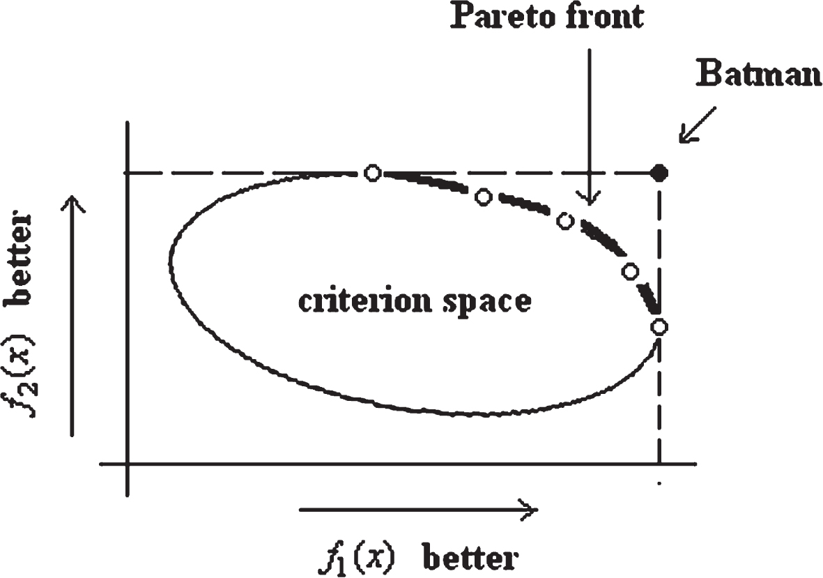
Consider the problem of finding a solution (player) according to (1). While Batman may not exist, a collection of players may be identified that cannot be bettered, or dominated, according to the c criteria. A player x*∈ ℵ is said to dominate another player x provided the following two conditions are met:
(2)
A player is said to be Pareto optimal provided they are not dominated by any other player in ℵ. The set of Pareto optimal players constitutes the Pareto optimal set (POS). The corresponding criteria vectors f(x) comprise the Pareto front (PF). An overview of Pareto-related concepts is available in Coello Coello et al. (2007).
By definition, the Pareto optimal set is defined as those players that are not Pareto dominated in the sense of (2). Thus, the POS can be generated by first forming the complement POSc, which is the set of dominated players. This is done in the following steps:
(3)
The steps in (3) identify the set POSc, so that POS=(POSc)c is the set of non-dominated solutions or the Pareto optimal set. The Pareto front consists of f(x) for all x ∈ POS.
Figure 1 shows two performance criteria values f1 and f2 so that c = 2. Batman corresponds to that player who simultaneously maximizes both criteria. The Pareto optimal set consists of the players lying on the boundary of the criterion space closest to Batman. This boundary forms the Pareto front. There are two points which lie on an axis. These players maximize either f1 or f2. Note that none of the Pareto optimal players can bettered in one criterion without deteriorating in the other criterion. If the two criteria are highly positively correlated, then the Pareto front will likely consist of only a few players. Otherwise, the criteria conflict and the Pareto front will then likely consist of numerous players.
Fig. 1
Illustration of the Pareto front and utopia point (Batman) in a two-criteria maximization problem.
2.2Scoring
A popular approach for finding an optimal solution to (1) is weighted aggregation as identified by Ngatchou et al. (2005) or the weighting method as identified by Ardakani and Wulff (2013). In this approach, all c criteria are combined to form a single objective function. The optimization problem is thus reduced to one function from which a batter can be scored and an optimal batter can be identified from this score. In particular, the formulation for weighted aggregation can be expressed as
(4)
A naive approach is to let ki(x) = fi(x). The sabermetrician can prespecify the weights according to their preferences, and rank players accordingly. However, the criteria could be on different scales which leads to the scaling problems mentioned previously. One approach to deal with differences in scales, and which is consistent with player rankings, is to let ki(x) = - ri(x) where ri(x) denotes the rank of player x∈ ℵ. with respect to criterion i. Then weights can be assigned in relation to the importance that is to be placed upon the rankings for criterion i. However, the use of rankings can mask differences of magnitude within the criteria values between players. In this study, players with ties in their criterion values are assigned the maximum of the ranks.
It is also possible to use (4) to assess the distance a player is from Batman, or from the hypothetical hitter xu who maximizes each criterion value separately. Marler and Arora (2004) recommend that the criteria be on the same scale before measuring distance. In particular, these authors consider the two scalings:
(5)
(6)
Equation (5) is the ratio between a player and Batman for criterion i. Equation (6) represents the desirability between a player and Batman for criterion i where xl denotes the hypothetical player with lowest criterion value in each of the criterion. This is the opposite of Batman, or the Joker. Thus, (6) compares the difference of a player from Joker relative to the difference of Batman from Joker for criteria i. As previously mentioned, equation (4) can be generalized using a power p to represent a weighted p-norm metric. Equation (4) assumes p = 1 which corresponds to the 1-norm or sum norm. Thus, (5) can be interpreted as the sum norm distance a player is to 0 relative to Batman. Equation (6) can be interpreted as the sum norm distance a player is to Joker relative to Batman.
As previously mentioned, a disadvantage of weighted aggregation is that it depends upon the selected weights {wi}. An experienced sabermetrician would pre-specify weights according to the specific objectives of the player performance evaluation. If there is no justified apriori rationale for specifying the weights, then equal weights could be used with wi = 1/c for i = 1, …, c. Equal weighting amounts to finding the average of the criteria.
In this study, there was no rationale for pre-speci-fying the weights. Thus, the weights were determined objectively using exploratory factor analysis (EFA). EFA hypothesizes a model in which the criteria are a linear combination of unobserved factors and coefficients in this model, or loadings, that are estimated to approximately reproduce the covariance matrix among the criteria (Rencher, 2012, pp. 435–441). A single factor model is hypothesized in this study, where that factor represents player performance. The loadings are estimated using maximum likelihood (Rencher, 2012, pp. 452), and then standardized to obtain the weights {wi} used in (4). The loading equals the covariance between the corresponding criterion and the factor representing player performance (Rencher, 2012, pp. 440). Thus, the higher the loading, the higher the weight for that criterion since it is most linearly related to player performance. The weights from the EFA approach are used for both the scoring in (4) and scored ratio to Batman in (5).
3Primary Pareto Optimal Set
MLB hitting data for 2016 is taken from baseballguru.com which has annual hitting data in EXCEL files under the player forecast section. Abbreviations for various performance variables are given in Table 1 for convenience. As in Koop (2002), pitchers and hitters with few AB are removed from the dataset. The removal of pitchers results in 620 hitters. Hitters with fewer than 60 AB are also removed to focus on full time hitters and to eliminate possible anomalies. The cut off of 60 AB is close to the first quartile of AB for the 620 hitters (65 AB). The final data set consists of n = 473 hitters. The hitting measures considered here are given by the six performance variables (y) in Table 1. These are the traditional well-known statistics to assess offensive performance, and are listed on popular baseball websites such as mlb.com. These statistics measure various aspects of offensive performance, including the ability of a hitter to get on base, generate runs, and hit for power. These criteria are also used in specific aggregations to formulate several sabermetrics. To avoid concerns with using the counting statistics (R, H, HR, RBI), these values are scaled by AB as recommended by Grabiner (2014).
Table 1
Baseball abbreviations for variable names (n), performance variables (y), sabermetric variables (s), predictor variables (x)
| Variable | Description |
| n1= AB | At Bat |
| n2= BB | Base on Balls |
| n3= CS | Caught Stealing |
| n4= H | Hits |
| n5= HR | Home Runs |
| n6= MVP | Most Valuable Player |
| n7= PA | Plate Appearance |
| n8= R | Runs Scored |
| n9= RBI | Runs Batted In |
| n10= ROY | Rookie of the Year |
| n11= SB | Stolen Base |
| n12= SF | Sacrifices |
| n13= SS | Silver Slugger |
| n14= TB | Total Bases |
| y1= Rr = R/AB | Runs per At Bat |
| y2= HRr = HR/AB | Home Runs per At Bat |
| y3= RBIr = RBI/AB | Runs batted In per At Bat |
| y4= AVG = H/AB | Batting Average |
| y5= OBP = (H + BB + HBP)/(AB + BB + HBP + SF) | On Base Percentage |
| y6= SLG = TB/AB | Slugging Percentage |
| s1= wOBA | Weighted On-base Average |
| s2= wRC+ | Weighted Runs Created Plus |
| s3= WAR | Wins Above Replacement |
| x1= G | Games Played In |
| x2= AB | At Bats |
| x3= AGE | Player Age |
| x4,j4= TEAM (reference = COL) | Team of Player |
| x5,j5= FP1 (reference = 1B) | Player Fielding Position |
| x6,j6= BATS (reference = R) | Batting Side of Plate |
Table 2 shows the correlation matrix for the 2016 hitting performance measures for players in the candidate set ℵ. All correlations are positive. SLG is moderately correlated with all the hitting measures, including OBP. HRr is correlated with RBIr as expected. The highest correlation is 0.78 which is observed between AVG and OBP as well as HRr and SLG. These correlations are moderate and would result in only mild concerns about multicollinearity according to Kutner et al. (2004, pp. 406–410). It is expected that statistics that are highly correlated will be coherent or produce similar rankings of player performance. Thus, the presence of these correlations is not an impediment to this multi-criteria approach.
Table 2
Correlation matrix for the six hitting performance measures
| Rr | HRr | RBIr | AVG | OBP | SLG | |
| Rr | 1 | 0.3963 | 0.3485 | 0.4920 | 0.5918 | 0.6037 |
| HRr | 0.3963 | 1 | 0.7609 | 0.1384 | 0.2919 | 0.7769 |
| RBIr | 0.3485 | 0.7609 | 1 | 0.3567 | 0.4227 | 0.7595 |
| AVG | 0.4920 | 0.1384 | 0.3567 | 1 | 0.7791 | 0.6899 |
| OBP | 0.5918 | 0.2919 | 0.4227 | 0.7791 | 1 | 0.6593 |
| SLG | 0.6037 | 0.7769 | 0.7595 | 0.6899 | 0.6593 | 1 |
The Pareto optimal set of 2016 MLB hitters with respect to these six performance criteria is shown in Table 3. This collection of 19 hitters lie on the primary Pareto optimal set (POS1) since they are non-dominated according to (2) and as such cannot be bettered by any other hitter in the candidate set with respect to these criteria. Within the Pareto optimal set, players are ranked according to their scored rankings across the six performance criteria using the weights obtained from EFA. The weights determined from EFA for the 2016 data are 0.14 for Rr, 0.17 for HRr, 0.17 for RBIr, 0.15 for AVG, 0.15 for OBP, and 0.22 for SLG. The mythical Batman consists of a mixture of Sanchez (HRr, SLG), Trout (Rr, OBP), Ortiz (RBIr), and LeMahieu (AVG). All batters have a scored ratio to Batman using (5) and the EFA weights which ranges from 0.69 (LeMahieu) to 0.90 (Sanchez) for players in POS1.
Table 3
Pareto optimal hitters, Pareto Front shown as ranks, scored rankings, scored ratios to Batman, and comments related to the evaluation of player performance
| name | team | pos | bats | age | games | ab | Rr.R | HRr.R | RBIr.R | AVG.R | OBP.R | SLG.R | s.rank | r.rank | s.Batman | comment |
| Sanchez | NYA | C | R | 23 | 53 | 201 | 35 | 4 | 41 | 26 | [1] | 16.02 | [1] | 0.9018 | AL rookie 2 | |
| Arenado | COL | 3B | R | 25 | 160 | 618 | 10 | 21 | 2 | 53 | 44 | 4 | 20.74 | 2 | 0.8266 | NL MVP 5, SS |
| Trout | LAA | OF | R | 24 | 159 | 549 | [1] | 73 | 20 | 16 | [1] | 13 | 21.36 | 3 | 0.8311 | AL MVP, SS |
| Ortiz | BOS | 1B | L | 40 | 151 | 537 | 125 | 12 | [1] | 16 | 6 | 2 | 23.45 | 4 | 0.8645 | Best Hitter, AL MVP 6, SS |
| Votto | CIN | 1B | L | 32 | 158 | 556 | 15 | 77 | 35 | 6 | 2 | 13 | 25.2 | 5 | 0.8017 | NL MVP 7 |
| Cabrera | DET | 1B | R | 33 | 158 | 595 | 85 | 30 | 24 | 12 | 10 | 8 | 26.14 | 6 | 0.7963 | AL MVP 9, SS |
| Bryant | CHN | 3B | R | 24 | 155 | 603 | 3 | 28 | 47 | 58 | 19 | 10 | 26.92 | 7 | 0.7985 | NL MVP |
| Murphy | WAS | 2B | L | 31 | 142 | 531 | 46 | 101 | 7 | 2 | 13 | 3 | 27.71 | 8 | 0.8069 | NL MVP 2, SS |
| Donaldson | TOR | 3B | R | 30 | 155 | 577 | 2 | 29 | 39 | 85 | 8 | 14 | 28.87 | 9 | 0.8076 | AL MVP 4 |
| Freeman | ATL | 1B | L | 26 | 158 | 589 | 30 | 47 | 92 | 34 | 6 | 5 | 34.93 | 10 | 0.7769 | NL MVP 6 |
| Braun | MIL | OF | R | 32 | 135 | 511 | 78 | 42 | 32 | 27 | 37 | 17 | 36.84 | 12 | 0.7631 | NL MVP 24 |
| Rizzo | CHN | 1B | L | 26 | 155 | 583 | 68 | 61 | 13 | 58 | 18 | 16 | 37.02 | 13 | 0.7676 | NL MVP 4, SS |
| Blackmon | COL | OF | L | 29 | 143 | 578 | 6 | 83 | 140 | 8 | 22 | 11 | 45.67 | 15 | 0.7605 | NL MVP 26, SS |
| Story | COL | SS | R | 23 | 97 | 372 | 19 | 9 | 9 | 131 | 128 | 7 | 46.11 | 16 | 0.7978 | NL Rookie 4 |
| Encarnacion | TOR | 1B | R | 33 | 160 | 601 | 49 | 13 | 3 | 183 | 82 | 26 | 55.05 | 20 | 0.7844 | AL MVP 14 |
| Altuve | HOU | 2B | R | 26 | 161 | 640 | 37 | 174 | 107 | 4 | 10 | 24 | 60.33 | 24 | 0.7362 | AL MVP 3 |
| Turner | WAS | OF | R | 23 | 73 | 307 | 32 | 130 | 197 | 3 | 46 | 7 | 68.96 | 29 | 0.7345 | NL Rookie 2 |
| Joyce | PIT | OF | L | 31 | 140 | 231 | 5 | 52 | 23 | 289 | 7 | 109 | 81.83 | 36 | 0.7449 | Free Agent |
| LeMahieu | COL | 2B | R | 27 | 146 | 552 | 9 | 329 | 239 | [1] | 4 | 66 | 113.09 | 58 | 0.6928 | NL MVP 15 |
POS1 identifies many well-known hitters in MLB for 2016. In fact, POS1 identifies the 2016 hitting award winners including the AL MVP, NL MVP, Silver Sluggers, vote-getters for MVP, and vote-getters for ROY. As previously mentioned, this is one of the objectives of sabermetrics. Sanchez had an incredible rookie season and received the lowest scored rank of all hitters given his production in Rr, RBIr, SLG. He is also the closest to Batman. Ortiz, a veteran hitter who had a fantastic year, received the Best Hitter award which is well deserved given that he is the third closest to Batman and had more AB than Sanchez. Four COL players are in POS1 (Arenado, Blackmon, Story, LeMahieu) where they each rank highly in a couple of the performance measures. While these are good hitters, increased performance might be expected at a hitter friendly park such as Coors Field. Joyce, a free agent who plays in OAK for 2017, might be an unexpected hitter to be included in POS1. However, he ranks fifth in Rr. Of those who rank higher, Trout has lower HRr, Donaldson has lower RBIr, Bryant has lower OBP, and DeShields (Table 4) has lower values in all other categories. By the definition in (2), Joyce is non-dominated and so is included in POS1.
Table 4
Secondary Pareto optimal hitters, Secondary Pareto Front shown as ranks, scored rankings, scored ratios to Batman, and comments related to the evaluation of player performance
| name | team | posl | bats | age | games | ab | Rr.R | HRr.R | RBIr.R | AVG.R | OBP.R | SLG.R | s.rank | r.rank | s.Batman | comment |
| Cruz | SEA | OF | R | 35 | 155 | 589 | 62 | 8 | 30 | 71 | 60 | 36.77 | [11] | 0.7859 | AL MVP 15 | |
| Betts | BOS | OF | R | 23 | 158 | 672 | 16 | 109 | 50 | 11 | 65 | 19 | 44.85 | [14] | 0.7503 | AL MVP 2, SS |
| Beltre | TEX | 3B | R | 37 | 153 | 583 | 98 | 61 | 29 | 39 | 65 | 31 | 51.44 | [17] | 0.7425 | AL MVP 7 |
| Cano | SEA | 2B | L | 33 | 161 | 655 | 57 | 41 | 83 | 44 | 88 | 23 | 53.92 | [18] | 0.7428 | AL MVP 8 |
| Cespedes | NYN | OF | R | 30 | 132 | 479 | 105 | 27 | 27 | 101 | 67 | 25 | 54.58 | [19] | 0.7527 | NL MVP 8, SS |
| Diaz | STL | SS | R | 25 | 111 | 404 | 24 | 134 | 75 | 39 | 33 | 37 | 57.83 | 21 | 0.7231 | NL ROY 5 |
| Ramirez | BOS | 1B | R | 32 | 147 | 549 | 123 | 63 | [5] | 75 | 57 | 46 | 58.70 | 22 | 0.7453 | |
| Goldschmidt | ARI | 1B | R | 28 | 158 | 579 | 13 | 137 | 64 | 45 | [3] | 71 | 58.81 | 23 | 0.7359 | AL MVP 11 |
| Rodriguez | PIT | 1B | R | 31 | 140 | 300 | 58 | 39 | 14 | 141 | 107 | 37 | 62.47 | 25 | 0.7436 | |
| Machado | BAL | 3B | R | 23 | 157 | 640 | 52 | 46 | 107 | 53 | 112 | 23 | 63.10 | 26 | 0.7316 | AL MVP 5 |
| Martinez | DET | OF | R | 28 | 120 | 460 | 108 | 96 | 118 | 24 | 37 | 18 | 64.61 | 27 | 0.7185 | |
| Dozier | MIN | 2B | R | 29 | 155 | 615 | 36 | 15 | 74 | 152 | 128 | 15 | 65.47 | 28 | 0.7514 | AL MVP 13 |
| Seager | SEA | 3B | L | 28 | 158 | 597 | 113 | 82 | 60 | 107 | 49 | 57 | 75.90 | 31 | 0.7081 | AL MVP 12, SS |
| Naquin | CLE | OF | L | 25 | 116 | 321 | 66 | 123 | 179 | 47 | 28 | 32 | 78.87 | 32 | 0.6981 | AL ROY 3 |
| Toles | LAN | OF | L | 24 | 48 | 105 | 17 | 253 | 97 | 17 | 37 | 46 | 80.10 | 33 | 0.7012 | |
| Carpenter | STL | 3B | L | 30 | 129 | 473 | 33 | 118 | 137 | 134 | 20 | 46 | 81.19 | 34 | 0.7011 | |
| Ho Kang | PIT | 3B | R | 29 | 103 | 318 | 153 | 22 | 8 | 224 | 96 | 34 | 82.00 | 37 | 0.7418 | |
| Seager | LAN | SS | L | 22 | 157 | 627 | 42 | 136 | 261 | 21 | 46 | 35 | 91.12 | 41 | 0.6856 | NL ROY |
| Yelich | MIA | OF | L | 24 | 155 | 578 | 185 | 178 | 44 | 44 | 27 | 78 | 91.45 | 42 | 0.6851 | NL MVP 19, SS |
| Santana | CLE | 1B | B | 30 | 158 | 582 | 96 | 44 | 109 | 203 | 57 | 60 | 91.65 | 43 | 0.7032 | |
| Schimpf | SDN | 2B | L | 28 | 89 | 276 | 28 | 10 | 16 | 395 | 140 | 23 | 93.65 | 45 | 0.7513 | |
| Bradley | BOS | OF | L | 26 | 156 | 558 | 38 | 107 | 88 | 158 | 104 | 74 | 94.05 | 46 | 0.6928 | |
| Trumbo | BAL | OF | R | 30 | 159 | 613 | 92 | [2] | 33 | 218 | 253 | 23 | 94.54 | 47 | 0.7479 | AL SS |
| Kinsler | DET | 2B | R | 34 | 153 | 618 | 7 | 113 | 177 | 68 | 121 | 76 | 95.35 | 48 | 0.6945 | |
| Healy | OAK | 3B | R | 24 | 72 | 269 | 193 | 93 | 156 | 27 | 149 | 29 | 102.13 | 51 | 0.6850 | |
| Pearce | BAL | 1B | R | 33 | 85 | 264 | 201 | 86 | 187 | 68 | 31 | 69 | 104.58 | 53 | 0.6772 | |
| Bour | MIA | 1B | L | 28 | 90 | 280 | 262 | 70 | 21 | 177 | 55 | 92 | 107.19 | 54 | 0.6957 | |
| Davis | OAK | OF | R | 28 | 150 | 555 | 94 | 3 | 18 | 265 | 303 | 29 | 108.31 | 55 | 0.7414 | |
| Harper | WAS | OF | L | 23 | 147 | 506 | 44 | 100 | 43 | 283 | 16 | 155 | 109.42 | 56 | 0.6904 | |
| Napoli | CLE | 1B | R | 34 | 150 | 557 | 48 | 34 | 25 | 306 | 161 | 105 | 109.90 | 57 | 0.7089 | |
| Dahl | COL | OF | L | 22 | 63 | 222 | 8 | 228 | 298 | 16 | 82 | 53 | 116.90 | 67 | 0.6727 | |
| Rosales | SDN | 3B | R | 33 | 105 | 214 | 31 | 35 | 65 | 351 | 216 | 66 | 120.91 | 72 | 0.7019 | |
| Bautista | TOR | OF | R | 35 | 116 | 423 | 70 | 79 | 68 | 333 | 55 | 132 | 122.03 | 74 | 0.6811 | |
| Carter | MIL | 1B | R | 29 | 160 | 549 | 95 | 6 | 41 | 374 | 225 | 57 | 123.68 | 78 | 0.7164 | |
| Ross | CHN | C | R | 39 | 67 | 166 | 137 | 37 | 10 | 351 | 88 | 148 | 125.58 | 80 | 0.6989 | |
| Segura | ARI | 2B | L | 26 | 153 | 637 | 72 | 230 | 326 | 9 | 49 | 57 | 125.84 | 81 | 0.6535 | NL MVP 13 |
| Vargas | MIN | 1B | B | 25 | 47 | 152 | 21 | 23 | 191 | 346 | 161 | 53 | 127.03 | 83 | 0.6969 | |
| Davis | BAL | 1B | L | 30 | 157 | 566 | 26 | 19 | 115 | 378 | 169 | 115 | 133.77 | 95 | 0.6913 | |
| Grandal | LAN | C | B | 27 | 126 | 390 | 254 | 14 | 17 | 354 | 141 | 86 | 134.00 | 96 | 0.7012 | NL MVP 22 |
| Pedroia | BOS | 2B | R | 32 | 154 | 633 | 45 | 293 | 248 | 11 | 37 | 138 | 135.83 | 102 | 0.6409 | |
| Swanson | ATL | SS | R | 22 | 38 | 129 | 83 | 297 | 190 | 34 | 24 | 154 | 136.99 | 103 | 0.6372 | |
| Fowler | CHN | OF | B | 30 | 125 | 456 | 12 | 254 | 308 | 115 | 16 | 142 | 148.11 | 117 | 0.6391 | |
| Hazelbaker | STL | OF | L | 28 | 114 | 200 | 25 | 39 | 146 | 331 | 333 | 83 | 152.81 | 126 | 0.6752 | |
| Rivera | NYN | 2B | R | 27 | 33 | 105 | 409 | 253 | 97 | [5] | 128 | 91 | 156.73 | 134 | 0.6358 | |
| Maybin | DET | OF | R | 29 | 94 | 349 | 11 | 399 | 224 | 16 | 24 | 209 | 159.43 | 138 | 0.6279 | |
| Zunino | SEA | C | R | 25 | 55 | 164 | 400 | 7 | 12 | 420 | 245 | 96 | 180.10 | 155 | 0.6745 | |
| Recker | ATL | C | R | 32 | 33 | 90 | 458 | 308 | 55 | 107 | 13 | 175 | 182.33 | 158 | 0.5976 | |
| Peraza | CIN | SS | R | 22 | 72 | 241 | 367 | 391 | 312 | 8 | 112 | 231 | 239.71 | 243 | 0.5553 | |
| DeShields | TEX | OF | R | 23 | 74 | 182 | [4] | 310 | 428 | 417 | 414 | 419 | 342.85 | 375 | 0.4991 |
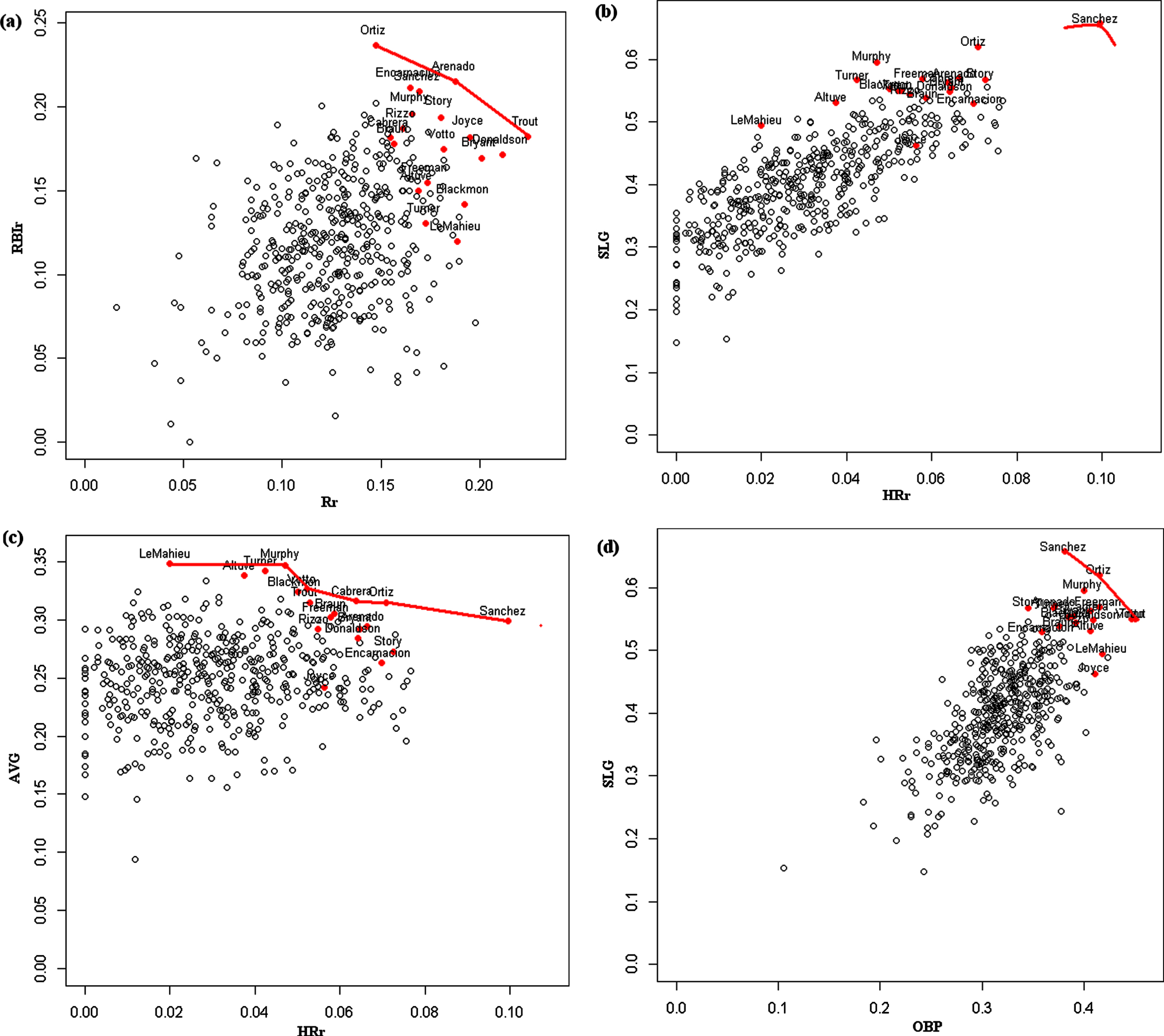
The multi-criteria approach is also helpful for learning about trade-offs among the criteria. Figure 2 shows plots involving just two criteria which can be compared to the idealized plot in Fig. 1. The criteria HRr and SLG have the second highest correlation (Table 2) which is evident by the linear relationship shown in Fig. 2 (b). Based upon just these two criteria, a reduced POS (POSr) would just consist of Sanchez, who is also the reduced Batman. Nevertheless, other POS1 hitters are rather scattered throughout these two criteria. The criteria OBP and SLG have the sixth highest correlation (Table 2) and the linear relationship can be seen in Fig. 2 (d). Now, the POSr from just these two criteria would consist of Sanchez, Ortiz, and Trout. The POS1 hitters are all located in the upper right of the plot. There are indications that SLG and OBP are redundant statistics in identifying these best hitters. The criteria Rr and RBIr have the third smallest correlation (Table 2) as is evident by the larger cloud of points in Fig. 2 (a). The POSr consists of a longer front than that in Fig. 2 (d) which contains Ortiz, Arenado, and Trout. Even though the POS1 hitters are all located in the upper right of the plot, the criteria values are also more spread out than they are in Fig. 2 (d). The criteria HRr and AVG have the smallest correlation (Table 2) as might be expected given the differences between power hitters and base hitters. Due to this conflict, the PF shown in Fig. 2 (b) is the longest, and the POSr consists of the six hitters LeMahieu (more of a base hitter), Murphy, Votto, Cabrera, Ortiz, and Sanchez (more of a power hitter). The criteria HRr and AVG demonstrate the most conflict among any pair of these criteria.
Fig. 2
Plots of the Pareto front involving (a) Rr and RBIr, (b) HRr and SLG, (c) HRr and AVG, (d) OBP and SLG.
4Secondary Pareto Optimal Set
Another tier of hitters can be identified in a secondary Pareto optimal set (POS2). The second-tier players are non-dominated according to (2) using a restricted candidate set in which the POS1 players are first removed, or ℵ2 = ℵ - POS1. The POS2 in this section is developed from the same MLB hitting data considered in section 3 for the 2016 season which consists of the n = 473 hitters, but without the 19 hitters on POS1 identified in Section 3.
POS2 is shown in Table 4 and consists of 49 well known hitters where the scored ratio to Batman ranges up to 0.79 (Cruz) and down to 0.50 (DeShields). POS 2 also identifies several award winners which is consistent with one of the objectives of sabermetrics. POS2 contains the NL ROY (Seager), the AL ROY 3 (Naquin), and the NL ROY 5 (Diaz). It also contains 5 Silver Slugger award winners (Betts, Cespedes, Seager, Yelich, Trumbo) along with various other hitters who received MVP votes. POS2 notably also contains a number of well-known hitters including Beltre (2004, 2010, 2011, 2014 SS), Goldschmidt (2013, 2015 NL MVP 2 and SS), Cano (2005 AL ROY 2 and 2006, 2010, 2011, 2012, 2013 SS), Machado (2015 AL MVP 4 and 2016 AL MVP 5), Harper (2012 NL ROY, 2015 NL MVP), Bautista (2010, 2011, 2014 SS), and Pedroia (2007 AL ROY, 2008 AL MVP and SS). These batters had good hitting seasons in 2016, but may not have received the same accolades as they did in previous seasons.
A few players have scored ratio to Batman greater than 0.75 (Cruz, Betts), and a few more have scored rankings in the top 19 (Beltre, Cano, Cespedes). POS2 contains players who have Rr ranked 4 (DeShields), HRr ranked 2 (Trumbo), RBIr ranked 5 (Ramirez), AVG ranked 5 (Rivera), OBP ranked 3 (Goldschmidt), and SLG ranked 9 (Cruz). While POS2 contains good hitters according to some of these metrics, these players are dominated by players in POS1 in terms of the other metrics. For example, Goldschmidt performs well in OBP, but is dominated by Trout and Votto. Trumbo hit the most HR in 2016 (47) which produces the second highest HRr (0.0767), but Sanchez has higher HRr (0.0995), and Sanchez dominates Trumbo in all other categories.
5Predicted Pareto Optimal Set
It is expected that particular hitters have an advantage to be Pareto optimal due to hitter friendly parks, team affiliations, or through regular playing time. Certain fielding positions are also reserved for the bigger and better hitters. A predicted Pareto optimal set (PPOS) can be constructed from multivariate predictions that are adjusted for these variables. The Multivariate Analysis of Variance (MANOVA) (Rencher and Christensen, 2012) is a tool that can be used to assess the predictor variable contributions and to obtain the predicted criteria values. Pareto optimality and weighted aggregation is then applied to these multivariate predicted values and the resulting uncertainty is propagated through the analyses using repeated sampling or the parametric bootstrap (Efron and Tibshirani, 1993, Section 6.5) from the predictive distribution.
The same MLB hitting data for 2016 is used here as that in sections 3 and 4. However, only qualifying hitters are included who meet the minimum plate appearance (PA) requirement of 502. For validation, MLB hitting data for 2017 is taken from baseballguru.com. There are 146 qualifying hitters for the 2016 season and 144 qualifying hitters for the 2017 season. Predictions are based upon the data from the 2016 season. The predictor variables (x variables) considered here are listed in Table 1. Factors, such as Team, Fielding Position, and Bats, include indicator variables for each level, except for the reference level (Kutner et al., 2004, pp. 313–324). The multiple criteria, or multiple response variables (y variables) are listed in Table 1 which can be denoted as the matrix Y. The partial Wilks’ Lambda test is conducted for the six predictors and for quadratic terms involving Age, G, AB to identify statistically important predictors. The test results are shown in Table 5 for the reduced model containing the statistically important predictors. Based upon these statistical test results, the predictions are based upon TEAM, FP1, BATS, AB, G, and G∧2 where the latter term denotes the quadratic trend in games played. Table 6 gives the estimated coefficients
Table 5
Partial MANOVA tests of the statistically important predictor variables using the Wilks’ Lambda test
| predictor | df | test stat | approx F | num Df | den Df | Pr(> F) |
| TEAM | 29 | 0.109 | 1.59 | 174 | 603 | < 0.0001 |
| FP1 | 5 | 0.500 | 2.56 | 30 | 406 | < 0.0001 |
| BATS | 2 | 0.661 | 3.87 | 12 | 202 | < 0.0001 |
| AB | 1 | 0.536 | 14.59 | 6 | 101 | < 0.0001 |
| G | 1 | 0.783 | 14.59 | 6 | 101 | 0.0003 |
| G∧2 | 1 | 0.766 | 5.15 | 6 | 101 | 0.0001 |
Table 6
MANOVA regression coefficient estimates
| predictor | Rr | HRr | RBIr | AVG | OBP | SLG |
| (Intercept) | 1.3121 | 0.4311 | 0.6549 | 0.4809 | 2.0755 | 0.4453 |
| TEAM ARI | –0.0178 | 0.0003 | –0.0199 | –0.0277 | –0.0250 | –0.0146 |
| TEAM ATL | –0.0392 | –0.0151 | –0.0371 | –0.0347 | –0.0423 | –0.0459 |
| TEAM BAL | –0.0353 | 0.0041 | –0.0335 | –0.0580 | –0.0746 | –0.0399 |
| TEAM BOS | –0.0163 | –0.0037 | –0.0052 | –0.0224 | –0.0238 | –0.0188 |
| TEAM CHA | –0.0545 | –0.0148 | –0.0375 | –0.0451 | –0.0550 | –0.0548 |
| TEAM CHN | –0.0098 | –0.0020 | –0.0100 | –0.0409 | –0.0154 | –0.0160 |
| TEAM CIN | –0.0252 | –0.0040 | –0.0235 | –0.0343 | –0.0461 | –0.0545 |
| TEAM CLE | –0.0193 | –0.0067 | –0.0253 | –0.0434 | –0.0420 | –0.0353 |
| TEAM DET | –0.0284 | –0.0013 | –0.0276 | –0.0265 | –0.0348 | –0.0436 |
| TEAM HOU | –0.0303 | –0.0118 | –0.0350 | –0.0341 | –0.0338 | –0.0455 |
| TEAM KCA | –0.0585 | –0.0109 | –0.0449 | –0.0573 | –0.0803 | –0.0617 |
| TEAM LAA | –0.0226 | –0.0141 | –0.0283 | –0.0189 | –0.0185 | –0.0552 |
| TEAM LAN | –0.0275 | –0.0094 | –0.0383 | –0.0297 | –0.0376 | –0.0293 |
| TEAM MIA | –0.0498 | –0.0203 | –0.0438 | –0.0221 | –0.0362 | –0.0557 |
| TEAM MIL | –0.0250 | 0.0069 | –0.0172 | –0.0377 | –0.0351 | –0.0449 |
| TEAM MIN | –0.0193 | 0.0012 | –0.0360 | –0.0559 | –0.0307 | –0.0365 |
| TEAM NYA | –0.0431 | –0.0120 | –0.0446 | –0.0383 | –0.0492 | –0.0550 |
| TEAM NYN | –0.0227 | 0.0193 | 0.0024 | –0.0374 | –0.0290 | –0.0204 |
| TEAM OAK | –0.0382 | –0.0027 | –0.0330 | –0.0413 | –0.0659 | –0.0502 |
| TEAM PHI | –0.0559 | –0.0152 | –0.0567 | –0.0406 | –0.0538 | –0.0576 |
| TEAM PIT | –0.0346 | –0.0130 | –0.0261 | –0.0293 | –0.0322 | –0.0433 |
| TEAM SDN | –0.0133 | –0.0139 | –0.0464 | –0.0621 | –0.0697 | –0.0384 |
| TEAM SEA | –0.0322 | 0.0057 | –0.0184 | –0.0355 | –0.0432 | –0.0326 |
| TEAM SFN | –0.0335 | –0.0157 | –0.0244 | –0.0379 | –0.0357 | –0.0413 |
| TEAM STL | –0.0307 | –0.0114 | –0.0282 | –0.0252 | –0.0193 | 0.0059 |
| TEAM TBA | –0.0497 | 0.0033 | –0.0254 | –0.0481 | –0.0660 | –0.0488 |
| TEAM TEX | –0.0301 | 0.0014 | –0.0122 | –0.0232 | –0.0406 | –0.0333 |
| TEAM TOR | –0.0268 | 0.0037 | –0.0108 | –0.0460 | –0.0397 | –0.0494 |
| TEAM WAS | –0.0183 | 0.0042 | 0.0044 | –0.0302 | –0.0168 | –0.0126 |
| FP1 2B | 0.0073 | –0.0158 | –0.0341 | –0.0010 | –0.0186 | –0.0352 |
| FP1 3B | 0.0088 | –0.0062 | –0.0191 | –0.0061 | –0.0132 | –0.0131 |
| FP1 C | 0.0010 | –0.0073 | –0.0180 | 0.0077 | –0.0010 | –0.0047 |
| FP1 OF | 0.0091 | –0.0075 | –0.0260 | –0.0135 | –0.0199 | –0.0295 |
| FP1 SS | –0.0085 | –0.0189 | –0.0394 | –0.0132 | –0.0324 | –0.0643 |
| BATS B | –0.0012 | –0.0043 | –0.0130 | 0.0116 | 0.0105 | 0.0050 |
| BATS L | 0.0014 | –0.0035 | –0.0095 | 0.0005 | 0.0087 | 0.0025 |
| AB | 0.0001 | 0.0001 | 0.0000 | 0.0004 | 0.0001 | 0.0006 |
| G | –0.0169 | –0.0059 | –0.0078 | –0.0039 | –0.0245 | –0.0288 |
| G∧2 | 0.000059 | 0.000022 | 0.000030 | 0.000009 | 0.000085 | 0.000098 |
It is also necessary to account for uncertainty in the predictions of future performance. This is accomplished using a parametric bootstrap where the performance criteria are obtained using replicate draws (REP) for each player
(5)
Validation of the predictions is performed using the data from the 2017 season. Table 7 shows the 19 players who are actually Pareto optimal (POS1) for the 2017 season. Uncertainty in the predictions is shown in the percent of replicate draws in which these players are predicted to be Pareto optimal (pPPOS1) and the 5%, 50%, 95% percentiles of the scored rankings from the replicate draws using the predictive distribution in (7). The criteria pPPOS1 provides a summary on a 0-1 scale where higher percentages denote a higher probability of that player being PPOS1. The ranking of the players in terms of pPPOS1 (pPPOS1r) is also shown in Table 7. The percentile intervals can be quite wide demonstrating large variability in the scored rankings across all of the criteria.
Table 7
Pareto optimal hitters along with covariate values, ranks of the performance criteria, and scored ratios to Batman for the 2017 season. Prediction information from the 2016 season is included using the proportion of time the player is predicted to be Pareto optimal (pPPOS1), player ranking in terms of pPPOS1 (pPPOS1r), and the 5%, 50%, 90% percentile values of the scored rankings from the parametric bootstrap. Comments are included to characterize the POS results
| nameLast | TEAM | FP1 | BATS | AGE | G | AB | Rr.R | HRr.R | RBIr.R | AVG.R | OBP.R | SLG.R | s.rank | r.rank | s.Batman | pPPOSl | pPPOSlr | 5% | 50% | 95% | comment |
| Trout | LAA | OF | R | 26 | 114 | 402 | 2 | 4 | 21 | 17 | 8 | 2 | 8.72 | 1 | 0.8357 | 0.156 | 43 | 10.00 | 64.00 | 122.00 | POS1 |
| Judge | NYA | OF | R | 25 | 155 | 542 | [1] | 2 | 5 | 46 | 9 | 3 | 10.24 | 2 | 0.8736 | NA | NA | NA | NA | NA | NA |
| Votto | CIN | 1B | L | 34 | 162 | 559 | 11 | 17 | 22 | 7 | 7 | 9 | 12.25 | 3 | 0.7718 | 0.182 | 31 | 5.00 | 41.50 | 113.95 | POS1 |
| Goldschmidt | ARI | 1B | R | 30 | 155 | 558 | 5 | 16 | 2 | 29 | 12 | 11 | 12.33 | 4 | 0.7887 | 0.370 | 2.00 | 20.00 | 82.95 | PPOS1, POS2 | |
| Stanton | MIA | OF | R | 28 | 159 | 597 | 6 | [1] | [1] | 51 | 23 | [1] | 12.50 | 5 | 0.8624 | NA | NA | NA | NA | NA | NA |
| Blackmon | COL | OF | L | 31 | 159 | 644 | 4 | 28 | 40 | 2 | 17 | 4 | 15.85 | 6 | 0.7635 | 0.410 | [5] | 2.00 | 26.50 | 91.00 | POS1 |
| Freeman | ATL | 1B | L | 28 | 117 | 440 | 9 | 18 | 41 | 15 | 11 | 6 | 16.51 | 7 | 0.7474 | 0.152 | 48 | 7.00 | 50.00 | 120.95 | POS1 |
| Arenado | COL | 3B | R | 26 | 159 | 606 | 33 | 23 | 3 | 13 | 29 | 6 | 16.66 | 8 | 0.7636 | 0.798 | [1] | 1.00 | 4.00 | 43.95 | PPOS1, POS1 |
| Zimmerman | WAS | 1B | R | 33 | 144 | 524 | 25 | 10 | 6 | 22 | 52 | 10 | 19.52 | 9 | 0.7638 | NA | NA | NA | NA | NA | NA |
| Cruz | SEA | OF | R | 37 | 155 | 556 | 37 | 8 | 4 | 40 | 28 | 13 | 20.28 | 10 | 0.7562 | 0.158 | 41 | 6.05 | 54.00 | 120.95 | POS1, PPOS2 |
| Ozuna | MIA | OF | R | 27 | 159 | 613 | 64 | 24 | 7 | 11 | 31 | 15 | 23.83 | 11 | 0.7329 | 0.020 | 115 | 37.05 | 107.50 | 143.00 | |
| Murphy | WAS | 2B | L | 32 | 144 | 534 | 20 | 69 | 24 | 5 | 19 | 17 | 25.95 | 14 | 0.7015 | 0.098 | 59 | 10.05 | 67.00 | 130.00 | |
| Rendon | WAS | 3B | R | 27 | 147 | 508 | 47 | 52 | 10 | 23 | 16 | 21 | 27.59 | 15 | 0.7086 | 0.302 | 17 | 3.00 | 28.00 | 91.95 | PROS2 |
| Altuve | HOU | 2B | R | 27 | 153 | 590 | 10 | 77 | 79 | 111 | 4 | 16 | 32.19 | 20 | 0.7783 | 0.222 | 25 | 6.00 | 40.00 | 114.95 | POS1 |
| Gonzalez | HOU | OF | B | 28 | 134 | 455 | 73 | 47 | 9 | 22 | 28 | 24 | 32.52 | 22 | 0.7002 | 0.114 | 54 | 11.05 | 61.00 | 124.95 | |
| Turner | LAN | 3B | R | 33 | 130 | 457 | 52 | 62 | 48 | 5 | 10 | 24 | 33.51 | 24 | 0.6797 | 0.074 | 70 | 13.00 | 72.00 | 133.00 | |
| Davis | OAK | OF | R | 30 | 153 | 566 | 44 | 6 | 13 | 117 | 6 | 26 | 33.56 | 25 | 0.8158 | 0.042 | 92 | 20.00 | 81.00 | 136.95 | POS2 |
| Alonso | SEA | 1B | L | 30 | 142 | 451 | 46 | 21 | 61 | 83 | 2 | 41 | 42.15 | 32 | 0.7555 | 0.036 | 100 | 23.05 | 89.00 | 140.00 | traded |
| Freese | PIT | 3B | R | 34 | 130 | 426 | 141 | 126 | 105 | 88 | [1] | 138 | 102.72 | 114 | 0.5888 | NA | NA | NA | NA | NA | NA |
Four of the players in Table 7 (Judge, Stanton, Zimmerman, and Freese) are not qualifiers in the 2016 season and so do not have predictions. Goldschmidt, Blackmon, and Arenado are on the actual POS1 for 2017 and are in the top 10 in terms of pPPOS1 based upon the 2016 predictions. The percentile intervals for these players contain low scored rankings. In particular, Arenado is predicted to be POS1 in nearly 80% of the replicate draws and 90 percent of his scored rankings are between 1 and 44. Arenado and Blackmon likely have high predictions since they play for COL. Goldschmidt and Rendon are POS1 for 2017 and also have pPPOS1 values greater than 0.3. These predictions are helpful since these players are not POS1 for 2016 as shown in Table 3. Cruz and Altuve are POS1 for 2017 and these players do have a relatively high pPPOS1 of 0.158, and 0.222, respectively.
As would be expected, not all players on POS1 for 2017 are predicted well based upon just the 2016 performance data. Ozuna, Murphy, Turner, Gonzalez, Davis, Alonso had surprising seasons in 2017, even though pPPOS1 for Gonzalez and Murphy is about 0.1. The scored rankings of Ozuna and Trout for 2017 do not fall within the 90% percentile interval based upon the predictions. The pPPOS1 values are 0.156 for Trout and 0.182 for Votto which do not rank overly high even though they are POS1 for 2017. The prediction model penalizes Trout in terms of R, HR, SLG and penalizes Votto in terms of AVG, OBP, SLG, so that these players perform better than expected according to the predictions. On the other hand, there are some players in the top 10 of pPPOS1 from the 2016 predictions who are not POS1 for 2017. Cabrera of DET (pPPOS1 = 0.372), Cano of SEA (pPPOS1 = 0.338), Gonzalez of COL (pPPOS1 = 0.412) each spent time on the disabled list in 2017. Such injuries may have impacted their 2017 season and some of these players did not perform as well as expected. Betts of BOS has a high pPPOS1 of 0.554, but had a disappointing 2017 season, particularly in terms of AVG and OBP. Encarnacion (CLE) and Rizzo (CHN) also have high pPPOS1 values of 0.468 and 0.386, respectively. While they do not appear on POS1 for 2017, they do appear on POS2 for 2017. Thus, their performance was good, even though it may not have been as good as predicted.
6Pareto Optimal Set with Other Criteria
It is important to recognize that the proposed multi-criteria approach can be easily implemented with any collection of criteria that a manager believes best characterizes player performance. This is the first advantage of the proposed multi-criteria approach mentioned in section 1. However, selection of the criteria is critical in that it must represent the player performance characteristics that are of specific interest to the performance assessment. A few considerations are presented below when it comes to thinking about the multiple criteria and how they compare to some popular sabermetrics. The multi-criteria approach is also demonstrated in this section using wOBA, wRC+, and WAR.
The multiple criteria previously considered are the widely available traditional measures of batting performance (R, HR, RBI, H, OBP, SLG). There are concerns about these traditional hitting statistics. Even though Grabiner (2014) mildly endorses AVG, it has been criticized by some, such as Albert (2010), for not addressing other ways to get on base, and for not distinguishing the type of hit. The statistics R and RBI have been criticized because they depend upon other factors that may not directly reflect player contribution such as scoring off the hit of another batter or needing to have runners on base (Grabiner 2014). Albert (2010) presents strong arguments that better measures of hitting are OBP, SLG, and OPS. On the other hand, rather than focusing on arguments that a statistic is flawed, it can be informative to recognize that statistics measure different aspects of hitting that cannot be captured in a single sabermetric. As stated by Grabiner (2014), “Batting average does fairly well because it counts hits, but it ignores power and walks, which are also important.” That point does not necessarily mean AVG is flawed, but that it measures a different aspect of hitting than does OBP or SLG. An advantage of the multi-objective approach is in its ability to work with a multitude of statistics that account for different aspects of player performance and for its ability to evaluate the trade-offs among these different aspects. This is the third advantage of the multi-criteria approach that is mentioned Section 1.
Concerns about traditional hitting statistics could lead a sabermatrician to apply the proposed approach with a different set of hitting performance measures. Some popular sabermetric statistics can be formulated from (4). In particular, this includes the following:
(8)
Another more complicated statistic, which is similar in form to SecA, is Weighted On-Base Average (wOBA) that is scaled by PA rather than AB. In particular, OPS is touted by Albert (2010) as a modern sabermetric. Yet, OPS is merely a specific weighted aggregation of OBS and SLG. However, this may not the best combination of OBP and SLG to represent hitting performance for a particular group of hitters. For example, Grabiner (2014) mentions the linear combination should be 1.2×OBP + SLG where the value 1.2 is usually ignored. The second advantage of the multi-criteria approach mentioned in section 1 is that such combinations and weights do not have to be specified as the performance in terms of OBP and SLG can be simultaneously considered and evaluated.
Some managers have become quite accustomed to particular sabermetrics for measuring player performance. As mentioned previously, the multi-criteria approach can be applied to any collection of criteria. As a demonstration, consider the collection wOBA, wRC+, and WAR defined by Fangraphs (2018b). Weighted On-Base Average (wOBA) combines different aspects of hitting and weights them according to the actual run value. Weighted Runs Created Plus (wRC+) attempts to credit a batter for the value of a hitting outcome while controlling for park, league, and year effects. Wins Above Replacement (WAR) is designed to measure overall player contribution, beyond just hitting, by comparing team wins compared to a replacement player. The data for these three sabermetrics are taken from Fangraphs (2018a) for the 2016 season and contains 146 hitters who are qualifying hitters with more than 502 plate appearances (PA).
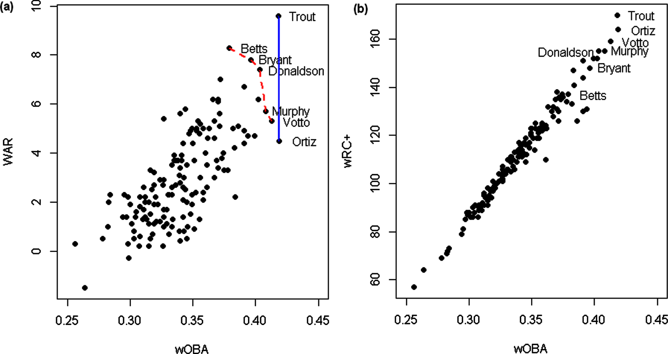
For these three sabermetrics, Table 8 gives the Primary Pareto optimal set (POSS1) and the Secondary Pareto optimal set (POSS2). The weights for these three criteria using EFA for the 2016 data were determined to be 0.36 for wOBA, 0.36 for wRC+, and 0.28 for WAR. The players are ordered in Table 8 according to the scored rankings. Ortiz is included on POSS1 since he had the highest observed wOBA which is slightly higher than that for Trout. If it were not for this value, then Trout would be the Batman with respect to these three criteria for which he still is very close (0.9991). POSS2 consists of Donaldson, Bryant, Murphy, Votto, and Betts. All these players are dominated by Trout and Ortiz who both have higher wOBA and wRC+ than any player on the secondary front. Figure 3 shows the players in POSS1 and POSS2 in terms of just two criteria. The pairwise correlation between wOBA and wRC+ is evident as expected since wRC+ is similar to wOBA, but controls for park, league, and year effects. Thus, player rankings for 2016 using wOBA are quite similar to those using wRC+. There is some conflict between wOBA and WAR since WAR measures additional player contributions beyond just hitting. The plot of wRC+ and WAR looks quite similar. The Pareto optimal sets POSS1 and POSS2 are much smaller than those presented in section 4 (POS1) and section 5 (POS2). This is due to fact that only three sabermetrics are used as the criteria and that two of these are highly correlated (0.9837). Nevertheless, all the players identified in POSS1 and POSS2 are included in POS1, except for Betts who is included in POS2. Betts is in POSS2 in large part due to his high value for WAR, which is the second highest.
Table 8
Primary and Secondary Pareto optimal hitters based upon the sabermetrics wOBA, wRC+, WAR listed in order of the scored ranking (s.rank)
| name | Team | G | PA | wOBA | wRC+ | WAR | s.rank | r.rank | s.Batman | POS |
| Trout | Angels | 159 | 681 | 0.418 | 170 | 9.6 | 1.36 | 1 | 0.9991 | primary |
| Donaldson | Blue Jays | 155 | 700 | 0.403 | 155 | 7.4 | 4.72 | 2 | 0.8903 | secondary |
| Murphy | Nationals | 142 | 582 | 0.408 | 155 | 5.7 | 6.60 | 3 | 0.8450 | secondary |
| Bryant | Cubs | 155 | 699 | 0.396 | 148 | 7.8 | 6.96 | 4 | 0.8812 | secondary |
| Votto | Reds | 158 | 677 | 0.413 | 159 | 5.3 | 7.20 | 6 | 0.8461 | secondary |
| Ortiz | Red Sox | 151 | 626 | 0.419 | 164 | 4.5 | 11.16 | 8 | 0.8385 | primary |
| Betts | Red Sox | 158 | 730 | 0.379 | 137 | 8.3 | 12.08 | 9 | 0.8578 | secondary |
Fig. 3
Plots of the players in terms of (a) wOBA and WAR, (b) wOBA and wRC+with labels for those players on the Primary and Secondary front. In (a), players on the Primary Pareto front are connected with a solid line while players on the Secondary Pareto front are connected with a dotted line.
It should be noted that there are also concerns about the use of these sabermetrics since wOBA does not adjust for hitting friendly parks, wRC+ does not differentiate positions, and WAR may not be developed enough to conduct player rankings (Fangraphs, 2018b). On the other hand, players have been ranked based upon WAR by the Baseball-Reference (2018). Due to these types of concerns, Fangraphs (2018) recommend in their discussion of WAR that one “should always use more than one metric at a time when evaluating players”. The proposed multi-criteria approach conducts this very task conveniently and efficiently.
7Summary
A multi-objective approach is proposed in this paper that allows for informative comparisons of players in terms of multiple performance criteria, avoids complex combinations of the criteria into single metrics, and allows trade-offs among the criteria to be evaluated. The approach is demonstrated for evaluating baseball player batting performance through simultaneous consideration of multiple performance metrics. Traditional metrics, such as R, H, HR, RBI, AVG, OBP, SLG, are initially used for these evaluations. The primary Pareto optimal set (POS1) identifies those batters who are non-dominated or who cannot be beat with respect to these criteria. The secondary Pareto optimal set (POS2) identifies a second group of batters who are non-dominated apart from those batters in POS1.The Multiple Analysis of Variance (MANOVA) is used to generate predictions while also addressing the uncertainty in the predictions and the uncertainty associated with the criteria. The uncertainty can then be propagated to the Pareto optimal sets and to the scored rankings for predicting performance results in an upcoming season. Weighted rankings or the relative distance to the utopia point (Batman) are also shown to be helpful when it comes to ordering players with respect to the multiple criteria.
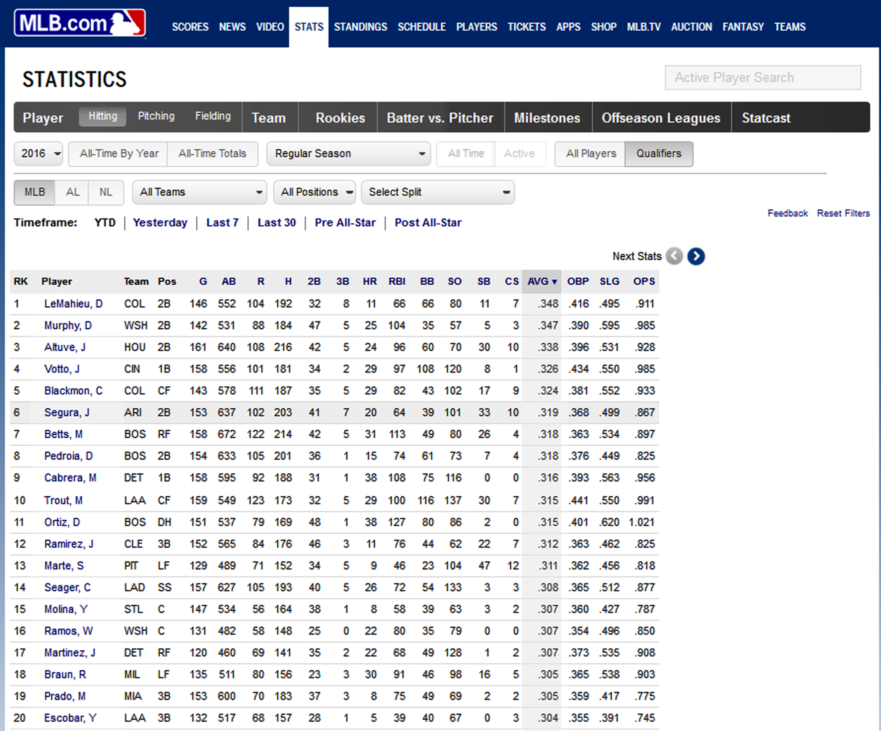
As an implementation example, the website mlb.com/stats contains statistics from which selected players can be ranked. Figure 4 shows a default view from this website for the 2016 MLB season. A few differences in the rankings can be observed from Fig. 4 and the previous rankings presented here due to their restriction to players who are qualifying hitters. However, simple adjustments to Fig. 4 can be made so that it can accommodate multiple criteria. That is, the user could be allowed to select multiple criteria items from among the hitting criteria such as R, HR, RBI, AVG, OBP, and SLG. Then the proposed calculations can be quickly applied so that players who are in POS1 are highlighted and players are then ordered according to their scored ranking across the criteria or according to their relative distance from Batman. As a result, Fig. 4 would more closely match that in Table 3.
The proposed approach is useful to casual fans, fantasy baseball players, and general managers for identifying the top players according to multiple criteria and to evaluate trade-offs among the criteria. The approach can be implemented rather easily with any collection of criteria that is perceived to best represent the type of player performance that is of interest. The criteria can be traditional, modern, or some combination. In addition, it is often necessary to fill out baseball rosters by position, in which case it makes more sense to implement the multi-criteria selection procedures separately for each position and likely with different criteria according to the expectations pertaining to that position. This approach could even involve a combination of hitting and fielding criteria. The proposed approach is also not limited to baseball. Baseball is often regarded as the sabermetric sport due to the wide availability of data, but other sports are now collecting various types of performance-based data. These multi-objective techniques would be useful tools to enhance sabermetrics.
Acknowledgments
The authors would like to thank the two anonymous referees for their suggestions and corrections that led to substantial improvements in the manuscript.
References
1 | Albert, J. , 2010, Sabermetrics: The Past, the Present, and the Future. URL: https://ww2.amstat.org/mam/2010/essays/AlbertSabermetrics.pdf. |
2 | Ardakani, M. K. and Wulff, S. S. , (2013) , An overview of optimization formulations for multiresponse surface problems, Quality and Reliability Engineering International, 29: , pp. 3–16. |
3 | Baseball-Reference. 2018, URL: https://www.baseball-reference.com/leaders/. |
4 | Coello Coello, C. A. , Lamont, G. B. and Van Veldhuizen, D. A. , (2007) , Evolutionary Algorithms for Solving Multi-Objective Problems, 2nd edn. New York: Springer. |
5 | Efron, B. and Tibshirani, R. J. , (1993) , An Introduction to the Boot-strap. New York: Chapman & Hall. |
6 | FanGraphs. 2018a, FanGraphs Leaders. URL: https://www.fangraphs.com. |
7 | FanGraphs. 2018b, FanGraphs Sabermetrics Library. URL: https://www.fangraphs.com/library/offense. |
8 | Grabiner, D. , 2014, The sabermetric manifesto. The Base-ball Archive. URL: https://seanlahman.com/baseball-archive/sabermetrics/sabermetric-manifesto/. |
9 | Koop, G. , (2002) , Comparing the performance of baseball players: A multiple-output approach, Journal of the American Statistical Association, 97: , pp. 710–720. |
10 | Kutner, M. H. , Nachtsheim, C. J. and Neter, J. , (2004) , Applied Linear Regression Models, 4th edn. Boston: McGraw Hill. |
11 | Marler, R. T. and Arora, J. S. , (2004) , Survey of multi-objective optimization methods for engineering, Structural Multidisciplinary Optimization, 26: , pp. 369–395. |
12 | Ngatchou, P. , Zarei, A. and El-Sharkawi, M. A. , (2005) , Pareto multi objective optimization, Proceedings of IEEE International Conference on Intelligent Systems ApplicationToPower Systems; Washington, DC, pp. 84–91. |
13 | Rencher, A. C. and Christensen, W. F. , (2012) , Methods of Multivariate Analysis, 3rd edn. Hoboken, NJ: Wiley. |


