
Who’s good this year? Comparing the information content of games in the four major US sports
Abstract
In all four major North American professional sports (baseball, basketball, football, and hockey), the primary aim of the regular season is to identify the best teams. Yet the number of regular season games used to distinguish between the teams differs dramatically between the sports, ranging from 16 (football) to 82 (basketball and hockey) to 162 (baseball). While length of season is partially determined by factors including travel logistics, rest requirements, playoff structure and television contracts, from a statistical perspective the 10-fold difference in the number of games between leagues suggests that some league’s games are more “informative” than others. In this paper, we propose a method to quantify the amount of information games yield about the relative strengths of the teams involved. Our strategy is to estimate a predictive accuracy curve which assesses how well simple paired comparison models fitted from X% of games within a season predict the outcomes of the remaining (100 - X)% of games, across multiple values of X. We compare predictive accuracy curves between seasons within each sport and across all sports, and find dramatic differences in the amount of information yielded by game results in the four major North American sports leagues.
1Introduction
In week 14 of the 2012 National Football League season, the New England Patriots squared off on Monday Night Football against the Houston Texans in a game with major implications for both teams. At the time, the Texans had the best record in the conference (11 wins versus 1 loss) and were in line to earn home-field advantage throughout the playoffs, while the New England Patriots (9 wins, 3 losses) had the best record in their division and were hoping to solidify their playoff position and establish themselves as conference favorites. The Patriots ultimately defeated the Texans 42-14, which led some commentators to conclude that the Patriots were the favorites to win the Super Bowl (Walker, 2012, MacMullan, 2012) and that Tom Brady was the favorite for the MVP award (Reiss, 2012). Others opined that the game provided evidence that the Texans were in reality less talented than they appeared over the first 13 weeks of the season (Kuharsky, 2012). These are strong conclusions to reach based on the results of a single game, but the power of such “statement games” is accepted wisdom in the NFL. In contrast, it is rare for the outcome of a single regular-season game to create or change the narrative about a team in the NBA, NHL, or MLB. While one might argue that the shorter NFL season simply drives commentators to imbue each game with greater metaphysical meaning, an alternative explanation is that the outcome of a single NFL contest actually does carry more information about the relative strengths of the teams involved than a single game result in the other major North American professional sports. In this paper, we ask and attempt to answer the basic question: how much does the outcome of a single game tell us about the relative strength of the two teamsinvolved?
In the four major North American professional sports (baseball, basketball, football, and hockey), the primary purpose of the regular season is to determine which teams most deserve to advance to the playoffs. Interestingly, while the ultimate goal of identifying the best teams is the same, the number of regular season games played differs dramatically between the sports, ranging from 16 (football) to 82 (basketball and hockey) to 162 (baseball). Though length of season is partially determined by many factors including travel logistics, rest requirements, playoff structure and television contracts, it is hard to reconcile the 10-fold difference in the number of games in the NFL and MLB seasons unless games in the former are somehow more informative about team abilities than games in the latter. Indeed, while it would be near-heresy to determine playoff eligibility based on 16 games of an MLB season (even if each of the 16 games was against a different opponent), this number of games is considered adequate for the same purpose in the NFL.
There is a well-developed literature on the topic of competitive balance and parity in sports leagues (Owen, 2010; Horowitz, 1997; Mizak et al., 2005; Lee, 2010; Hamlen, 2007; Cain and Haddock, 2006; Larsen et al., 2006; Ben-Naim et al., 2006; Késenne, 2000; Vrooman, 1995; Koopmeiners, 2012). However, most papers focus on quantifying the degree of team parity over consecutive years along with the effects of measures taken to increase or decrease it. In papers which compare multiple sports, season length is often viewed as a nuisance parameter to be adjusted for rather than a focus of inquiry. As a result, little attention has been directed at the question of how information on relative team strength accrues over the course of a single season.
In this paper, we aim to quantify the amount of information each game yields about the relative strength of the teams involved. We estimate team strength via paired-comparison (Bradley and Terry, 1952) and margin-of-victory models which have been applied to ranking teams in a variety of sports (McHale and Morton, 2011; Koehler and Ridpath, 1982; Sire and Redner, 2009; Martin, 1999). The growth in information about the relative strength of teams is quantified via a predictive accuracy curve which describes how paired-comparison models fitted from X% of the games in a season predict the outcomes of the remaining (100 - X)% of games, across multiple values of X (games are partitioned into training and test sets at random to reduce the impact of longitudinal trends over the course of a season). A predictive accuracy curve is also obtained for describing how paired-comparison models fitted from X number of games from a season predict the outcomes of the remaining games in the season, across multiple values of X. We begin by describing the data and analysis methods we used in Section 2. Section 3 presents results from recent seasons of the four major North American sports, and compares the “information content” of games across the four sports. In Section 4 we discuss the strengths and limitations of our analysis.
2Methods
2.1Data
We consider game results (home and away score) for the 2010-2015 seasons for the NFL, the 2010-2011 to 2015-2016 seasons of the NBA, the 2010-2011 to 2015-2016 seasons of the NHL, and the 2010-2015 seasons of MLB. Game results for the NFL, NBA and NHL were downloaded from Sports-Reference.com (Drinen, 2014) and game results for MLB were downloaded from Retrosheet (Smith, 2014). Only regular season games were considered in our analysis. A small number of tie games were removed from the data to simplify the fitting of models for binary win/loss outcomes, though we note that there are models that can accommodate tied game results (Rao and Kupper, 1967).
2.2Quantifying Informativeness
Let
(1)
We fit a similar model when the actual game scores are considered. In this context, home team margin of victory (MOV) Δg is recorded for each game; Δg is positive for a home team win and negative for a home team loss (as noted above, a small number of tie games with Δg = 0 were excluded from our analyses). The paired comparison model incorporating margin of victory is:
(2)
Both models (1) and (2) can be fit using standard statistical software, such as R (R Core Team, 2013). Given estimates
Our metrics for summarizing the amount of information on relative team strength are based on how well the results of games in G allow us to predict the outcomes of games in G′. Specifically, given G and G′, our information metric is the fraction of games in G′ which are correctly predicted using a paired comparison model applied to G:
For a given season, we estimated IBT and IMOV for sets of game results corresponding to 12.5%, 25.0%, 37.5%, 50.0%, 62.5%, 75.0% and 87.5% of the games in each available season. For a given season percentage X%, training data sets G1, G2, …, GK were formed by randomly sampling games corresponding to X% of that season, and test data sets
1. For X = 12.5, 25, 37.5, 50, 62.5, 75, and 87.5:
(a) Generate 100 training sets G1, G2, …, G100 (and complementary test sets
(b) For each training set Gk:
i. Fit models (1) and (2) to the games in Gk.
ii. Obtain binary win/loss predictions for the games in the test set
iii. Evaluate the information metrics
(c) Average the computed information metrics to estimate the predictive accuracy of paired comparison models fitted to data from X% of the entire season (IBT and IMOV).
2. Summarize IBT and IMOV across different values of X.
The above approach defines a predictive accuracy curve which quantifies how the ability to predict game outcomes changes as a higher proportion of the season’s games are used in a predictive model. Through a similar process, we produced a predictive accuracy curve which quantifies how the ability to predict game outcomes changes as a higher number of games from the season are used in the model.
2.3Information accrual rate
In addition to quantifying the accuracy of prediction models, we also sought to measure how quickly information accrued in each sport, i.e., how rapidly prediction accuracy improved as the number of games used to fit the prediction model increased. We therefore calculated a sport-specific information accrual rate based on the derivative of the IMOV curve. Specifically, we calculated the information accrual rate as follows:
1 Fit a fourth-degree (quartic) polynomial equation, via least squares, to the sport-specific values of IMOV for all years since 2010.
2 Compute the derivative of the fitted curves (a trivial task since the curve is defined by a polynomial) to define an instantaneous information accrual rate, i.e., the rate of change in IMOV for a prediction model using any given number of games or fraction of games in the season.
For the sake of brevity, we present information accrual rates for IMOV only; the same steps could easily be applied to compute information accrual on the basis of IBT. The fitted quartic polynomial curves and information accrual rate curves for the four sports are presented in Section 3. Model coefficients and their corresponding standard error estimates are provided in Tables A1 through A4 in Appendix A.
3Results
Figures 1 through 4 summarize the trajectories of IBT and IMOV for multiple seasons in each of the four major U.S. sports. The natural null model comparison for these curves is the “home-field advantage” (HFA) model which chooses the home team to win every game; in these plots, the predictive accuracy of the HFA model is represented by a horizontal solid line. The average win probability for the home team (as determined by the parameters α and λ in models (1) and (2) respectively) varies from approximately 53% to 61% across the four sports. The home team winning between 55% and 60% of NFL games, approximately 60% of NBA games, and between 50% and 55% of MLB and NHL games is consistent with previous studies of home-field advantage (Pollard and Pollard, 2005; Liardi and Carron, 2011).
Fig.1
Percent of games correctly predicted on test set vs. average number of games per team in training set, NFL seasons 2010-2015.
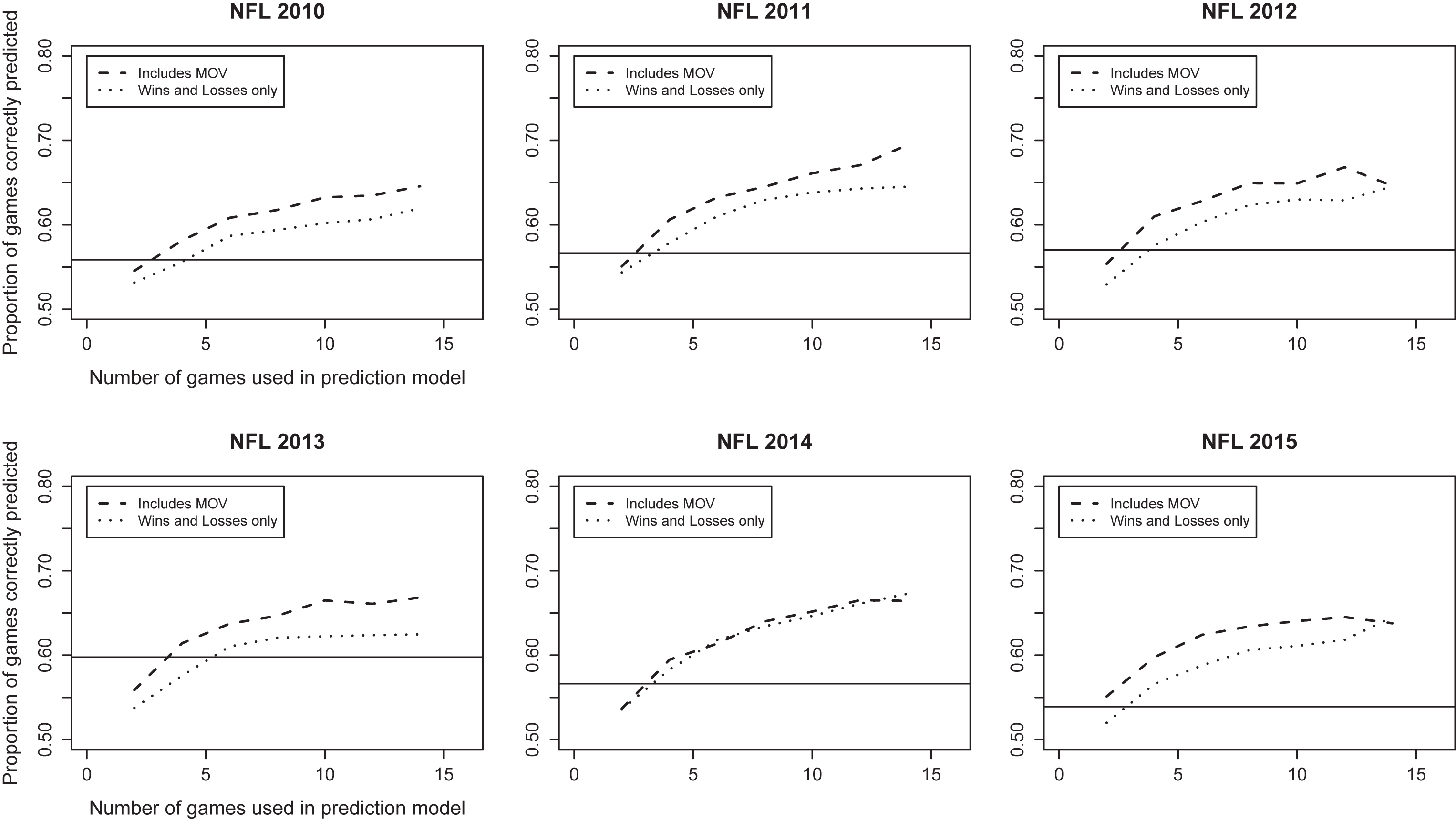
3.1National Football League
The percent of games correctly predicted on the test set versus the average number of games per team in the training set for the 2010-2015 National Football League seasons is displayed in Fig. 1. Both paired comparison models (i.e., those which incorporate and ignore margin of victory) outperform simply picking the home team to win every game. The margin of victory model appears to perform slightly better than the paired comparison model, though the differences are modest (and in the 2014 season, non-existent). The prediction accuracy of both models improves as the number of games used to make predictions increases, with the rate of increase in accuracy (i.e., information) being largest for the first 4-6 games per team included in the model. While the rate of increase in accuracy slows as additional games are added to the prediction model, it is notable that accuracy continues to increase even beyond 10-12 games in most years.
3.2National Basketball Association
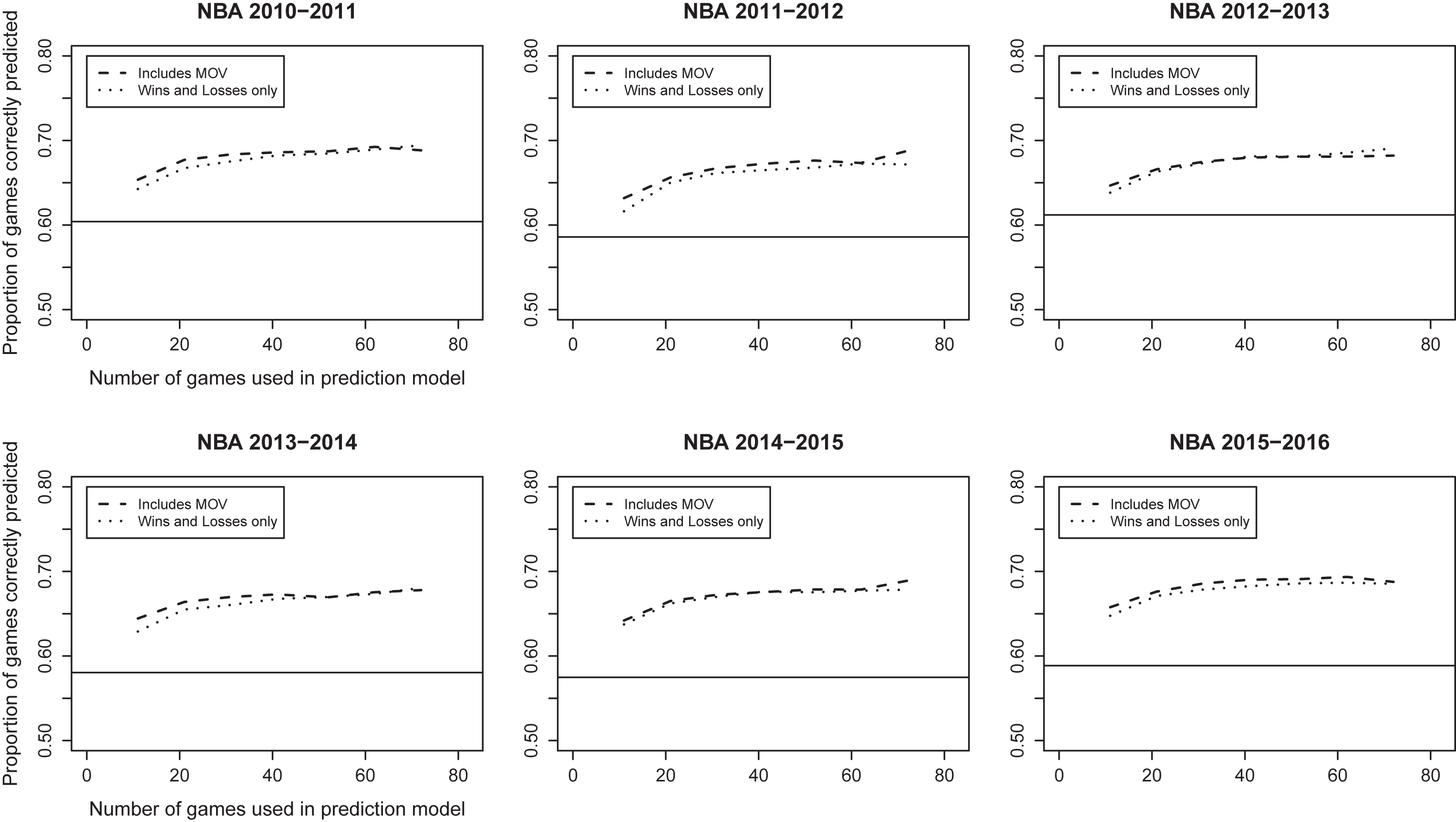
Results for the National Basketball Association can be found in Fig. 2. The NBA was the most predictable of the four major North American professional sports leagues. Using 87.5% of games as a training set, our model was able to predict with over 65% accuracy across seasons. The NBA also had the largest home court advantage with home teams winning approximately 60% of games. There was virtually no advantage in including margin of victory in our models. The only major difference between the NFL and NBA was the growth of information over the season. While the accuracy of our predictions for the NFL continued to improve as more games were added to the training set, model accuracy for the NBA did not improve substantially once more than 25% of games (i.e., ≥ 21 games per team) were included in the training set. Analyses using the segmented package in R for fitting piecewise linear models (Muggeo, 2003, 2008) confirmed an inflection point in the prediction accuracy curve when approximately 25-30 games per team were used in the model.
Fig.2
Percent of games correctly predicted on test set vs. average number of games per team in training set, NBA seasons 2011-2016.
3.3Major League Baseball and the National Hockey League
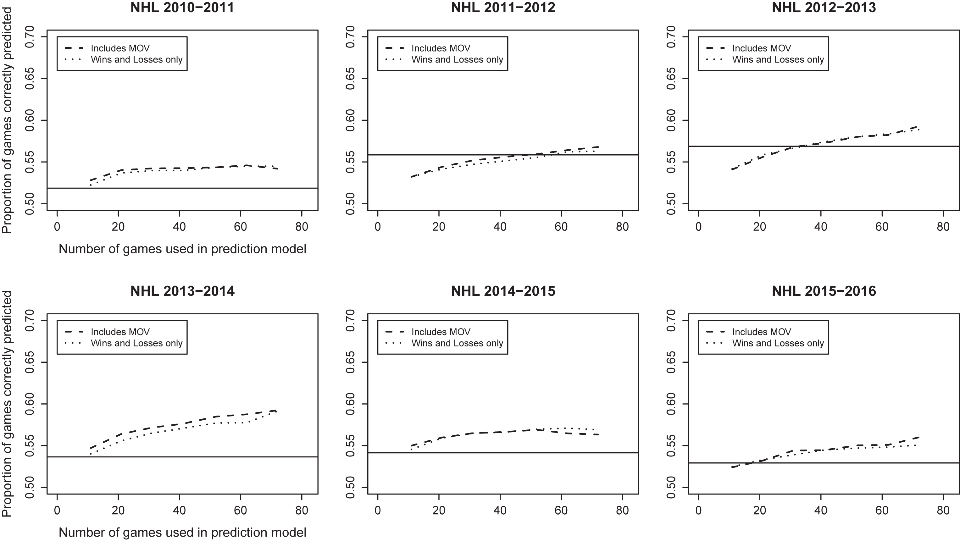
Results from Major League Baseball and the National Hockey League are found in Figs. 3 and 4, respectively. The results for MLB and the NHL were quite similar, in that both leagues were substantially less predictable than the NFL and NBA. The percentage of games correctly predicted for MLB never exceeded 58% even when 140 games (87.5% of a season) were included in the training set. The NHL was slightly better but our model was never able to predict more than 59% of games correctly. Prediction accuracy was rarely more than 2-3 percentage points better than the simple strategy of picking the home team in every game for either league. For example, the maximum predictive accuracy in the NHL was achieved in the 2012-2013 season when the home team win probability was relatively high at 57%. And, during the 2011-2012 season, picking the home team performed better than paired comparison models constructed using a half-season’s worth of game results.
Fig.3
Percent of games correctly predicted on test set vs. average number of games per team in training set, MLB seasons 2010-2015.
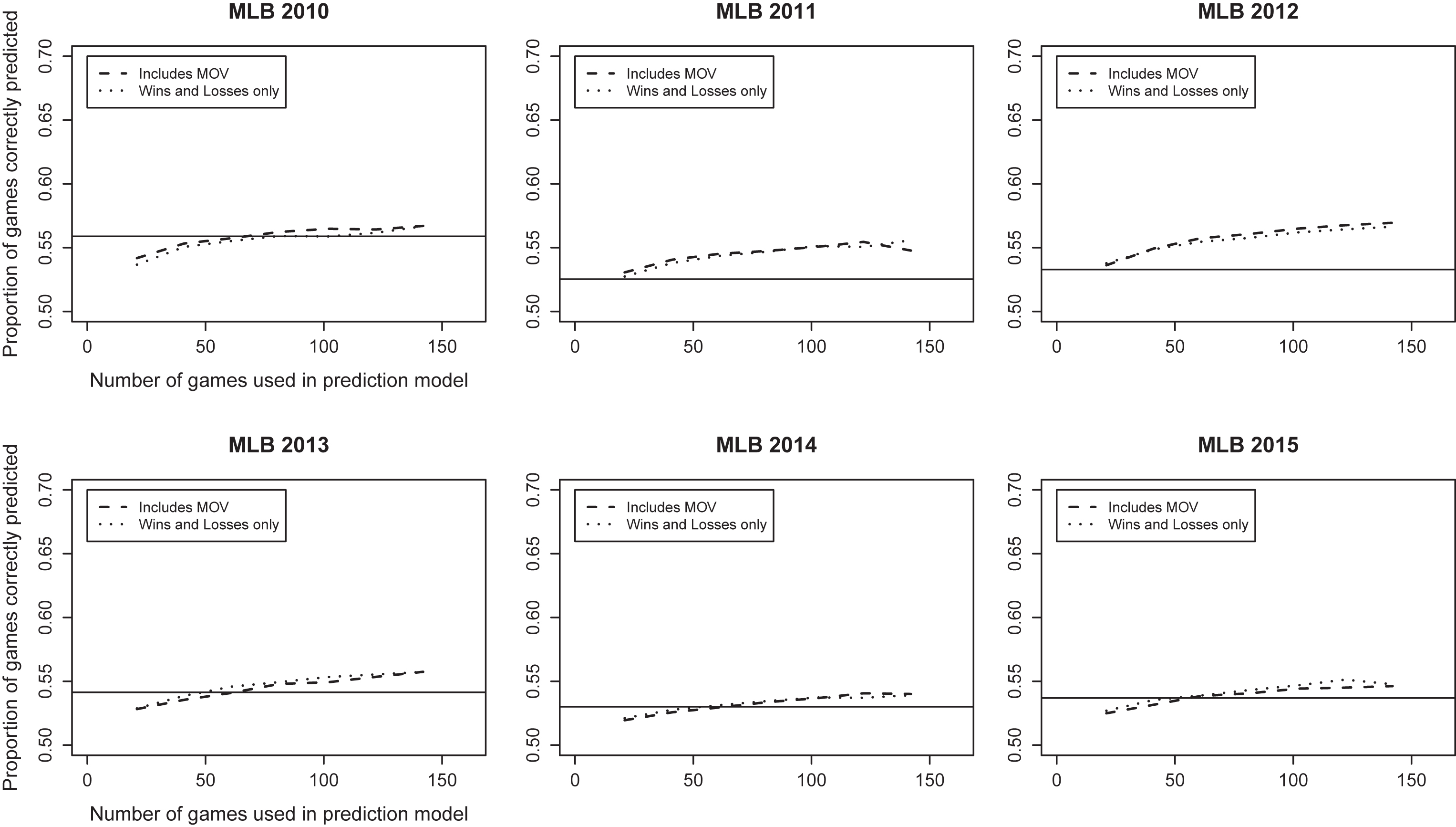
Fig.4
Percent of games correctly predicted on test set vs. average number of games per team in training set, NHL seasons 2011-2016.
3.4Comparing the sports
Here, we summarize and compare the predictive accuracy of the MOV model for the four major sports, aggregated across the years of available data. Results from the win-loss model were similar, and are not shown. Figure 5a is an aggregated version of the per-sport predictive accuracy plots, and summarizes predictive accuracy versus the number of games used in the training set. Figure 5b also plots predictive accuracy, but versus the proportion of games used in the training set. Information accrual rates (see Section 2.3) are summarized, per game and per proportion of games, in Figs 6a and 6b.
Fig.5
Proportion of games correctly predicted by margin of victory model (IMOV) for four major U.S. sports leagues. Lines are quartic polynomials fit to data from each sport aggregated across the years 2010-2016. (a) Information accrual rate by number of games used in prediction model. Number of games truncated at 41 for readability. (b) Information accrual rate by proportion of season games used in prediction model.
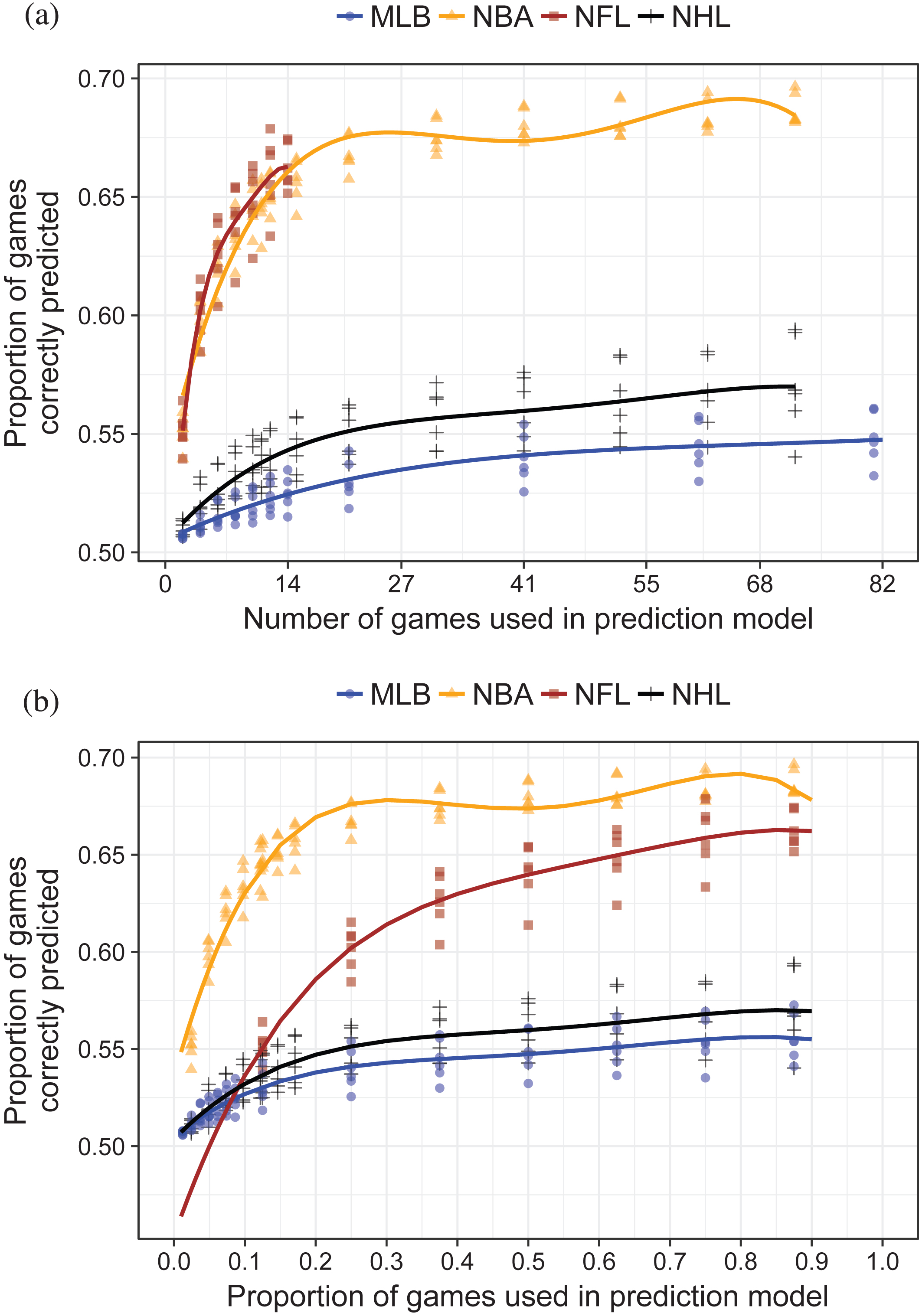
Fig.6
Information accrual rate (first derivative of IMOV curve) for four major U.S. sports leagues. (a) Information accrual rate by number of games used in prediction model. Number of games truncated at 41 for readability. (b) Information accrual rate by proportion of season games used in prediction model.
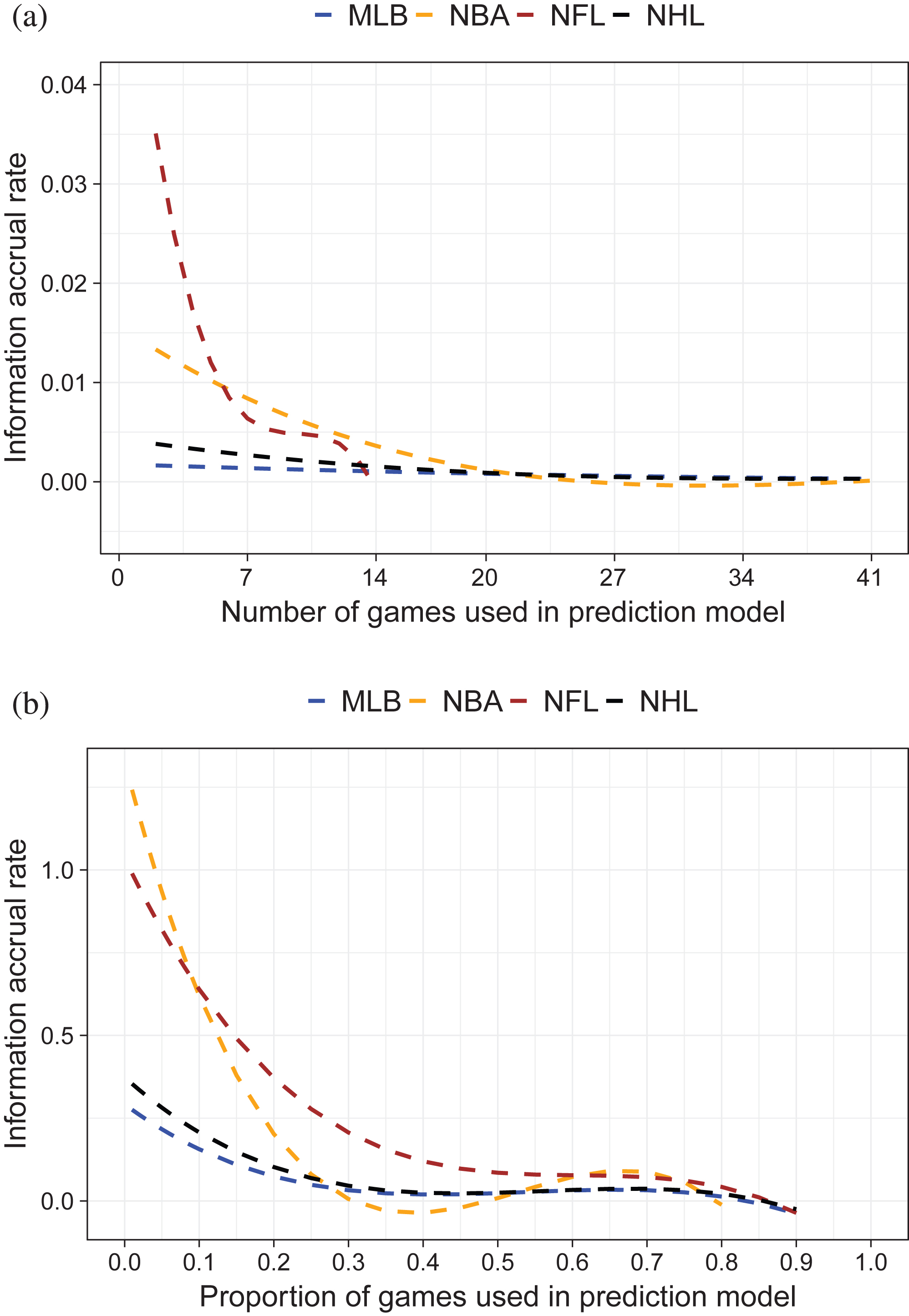
Figures 5a and 6a show that on a per-game basis, NFL games are most informative. Over the first five games (per team) used in the prediction model, prediction accuracy improves by at least 1% per game, with the most dramatic improvements (3-4% per game improvement rate) accruing after the initial 2-3 games. The initial 5-10 games of the NBA season offer more modest, but still substantial,improvements of approximately 1% accuracy per game. Initial NHL games are slightly more informative than initial MLB games, but the per-game improvements in predictive accuracy are below 0.5% and 0.2% respectively.
Figures 5b and 6b place data on the same horizontal scale, comparing predictive accuracy and information accrual rate as the proportion of games used in the prediction model varies. From Figure 6b, we see that the first 10-15% of games included in the NBA prediction model actually provide more information than the first 10-15% of games included in the NFL prediction model. However, the information accrual rate of NBA games quickly approaches zero beyond this point, while prediction model accuracy continues to improve in the NFL model beyond 50% of games. Indeed, at the point where 25% of games have been included in the prediction model, the information accrual rate of the NBA is very similar to that of the MLB and NHL (∼0.1%), while the NFL’s information accrual rate is more than 2.5 times higher (∼0.25%). Information accrues at a more modest rate for MLB and NHL games; for these two sports, as in the NBA, the accrual rate is essentially zero once 30% of the season’s games are included in the prediction model.
4Discussion
Our results reveal substantial differences between the major North American sports according to how well one is able to discern team strengths (and hence predict the outcomes of future games) using game results from a single season. NBA games are most easily predicted, with paired comparison models having good predictive accuracy even including a small fraction of the season; indeed, since our information metric for the NBA appears to plateau at around 25 games, a large fraction of games in the NBA season are superfluous from the point of view of distinguishing the best and worst teams in the league. NFL game results also give useful information for determining relative team strength. On a per-game basis, NFL contests contain the largest amount of information, and unlike in the other sports substantial information continues to accrue though the majority of the season’s games. While we randomly permuted the order of games when adding them to our prediction model instead of considering them in their scheduled order, our results suggest that for the NBA, NHL, and MLB, the first quarter of the season provides most of the information necessary for determining relative team strength, while games in the second half of the NFL season contribute useful information in determining the strongest teams.
The predictive ability of paired comparison models constructed from MLB and NHL game data remains limited even when results from a large number of games are used. One interpretation of this finding is that, in comparison to the NBA and NFL, games in MLB and the NHL carry little information about relative team strength. Our results may also reflect smaller variance in team strengths (i.e., greater parity) in hockey and baseball: Because our information metric considers the predictive accuracy averaged across all games in the test set, if most games are played between opposing teams of roughly the same strength then predictive models based only on paired comparisons will fare poorly. Indeed, the inter-quartile range for winning percentage in these sports is typically on the order of ∼20%, while in football and basketball it is closer to 30%.
Our observation that the hockey and baseball regular seasons do relatively little to distinguish between teams’ abilities is reflected in playoff results in these sports, where “upsets” of top-seeded teams by teams who barely qualified for the postseason happen much more regularly than in the NFL and NBA. Specifically, for the six seasons of available data lower-seeded teams won first-round playoff series 43.8% of the time in the NHL, and 58.3% of the time in MLB (Drinen, 2014, Smith, 2014). However, lower-seeded teams won only 25.0% of divisional round playoff games in the NFL, and 27.1% of first-round games in the NBA. While there are many considerations when designing playoff structures (Bojke, 2008), an argument could be made for increasing the number of teams that qualify for the MLB playoffs since the current 10-team format is likely to exclude teams of equal or greater ability than ones that make it. Using similar logic, one might also argue that perhaps the NBA playoffs are overly inclusive as there is ample information contained in regular season game outcomes to distinguish between the best teams and those that are merely average.
The enormous discrepancy in the informativeness of game results between hockey and basketball, which both currently play seasons of the same length, is notable. One possible explanation for why basketball game results more reliably reflect team strength is that a large number of baskets are scored, and the Law of Large Numbers dictates that each team approaches their “true” ability level more closely. In contrast, NHL games are typically low-scoring affairs, further compounded by the fact that a large fraction of goals are scored on broken plays and deflections which seem to be strongly influenced by chance. We have not analyzed data from soccer, but it would be interesting to explore whether the “uninformativeness” of hockey and baseball game results extends to other sports, or whether the relatively low parity of soccer makes individual games more “informative” according to our metrics.
Our analysis has several limitations. First, we chose to quantify information via the predictive accuracy of simple paired comparison models. It is possible that using more sophisticated models for prediction might change our conclusions, particularly for sports like the NBA where the predictiveness curve plateaus early. Nevertheless, we doubt that using more complex models would erase the sizable between-sport differences that we observed. One possible explanation for the fact that the outcome of a randomly chosen baseball game is hard to predict based on previous game results is the significant role that the starting pitcher plays in determining the likelihood of winning; the “effective season length” of MLB could be viewed as being far less than 162 games because each team-pitcher pair carries a different win probability. However, in additional analyses (results not shown), we fitted paired comparison models including a starting pitcher effect and this did not substantially affect our results. Second, it could be argued that team win probabilities change over the course of a season due to roster turnover, injuries, and other effects. By randomly assigning games to our training and test set without regard to their temporal ordering, we are implicitly estimating “average” team strengths over the season, and applying these to predict the outcome of an “average” game. We chose a random sampling approach over one which would simply split the season because we wanted to eliminate time trends in team strengths when describing how information accrued as more game results were used to build prediction models. Our approach therefore does not directly describe how predictive accuracy improves as games are played in their scheduled order.
Appendices
Appendix A
Table A1
Fitted coefficients for the quartic polynomial model
| League | β0 | β1 | β2 | β3 | β4 |
| MLB | 0.505 | 0.002 | –3.07E-05 | 2.46E-07 | –7.04E-10 |
| NBA | 0.537 | 0.016 | –6.25E-04 | 1.03E-05 | –5.91E-08 |
| NFL | 0.454 | 0.065 | –9.16E-03 | 6.26E-04 | –1.61E-05 |
| NHL | 0.504 | 0.004 | –1.40E-04 | 2.07E-06 | –1.11E-08 |
Table A2
Fitted coefficients for the quartic polynomial model
| League | β0 | β1 | β2 | β3 | β4 |
| MLB | 0.50 | 0.29 | –0.83 | 1.09 | –0.51 |
| NBA | 0.54 | 1.33 | –4.37 | 5.95 | –2.81 |
| NFL | 0.45 | 1.04 | –2.35 | 2.56 | –1.06 |
| NHL | 0.50 | 0.37 | –1.01 | 1.25 | –0.56 |
Table A3
Standard error estimates for coefficients of quartic polynomial model
| League | β0 | β1 | β2 | β3 | β4 |
| MLB | 2.71E-03 | 3.69E-04 | 1.14E-05 | 1.23E-07 | 4.30E-10 |
| NBA | 4.67E-03 | 9.56E-04 | 5.63E-05 | 1.20E-06 | 8.28E-09 |
| NFL | 3.10E-02 | 2.28E-02 | 5.30E-03 | 4.83E-04 | 1.50E-05 |
| NHL | 5.22E-03 | 1.07E-03 | 6.29E-05 | 1.34E-06 | 9.25E-09 |
Table A4
Standard error estimates for coefficients of quartic polynomial model
| League | β0 | β1 | β2 | β3 | β4 |
| MLB | 0.003 | 0.060 | 0.300 | 0.528 | 0.299 |
| NBA | 0.005 | 0.078 | 0.375 | 0.660 | 0.375 |
| NFL | 0.031 | 0.365 | 1.357 | 1.978 | 0.985 |
| NHL | 0.005 | 0.088 | 0.427 | 0.751 | 0.427 |
References
1 | Agresti A. , (2002) , Categorical Data Analysis, Wiley series inprobability and statistics, 2 edn, John Wiley & Sons. |
2 | Ben-Naim E. , Vazquez F. & Redner S. , (2006) , Parity and predictability of competitions, Quantitative Analysis in Sports, 2: (4), 1–12. |
3 | Bojke C. , (2008) , The impact of post-season play-off systems on theattendance at regular season games, in Albert J. and Koning R. H. ,eds, ‘Statistical Thinking in Sports’, Chapman & Hall/CRC Press, Boca Raton, FL, chapter 11, pp. 179–202. |
4 | Bradley R.A. and Terry M.E. , (1952) , Rank analysis of incomplete block designs: I. The method of paired comparisons, Biometrika. 324–345. http://www.jstor.org/stable/2334029 |
5 | Cain L.P. and Haddock D.D. , (2006) , Research notes: Measuring parity tying into the idealized standard deviation, Journal of Sports Economics, 7: (3), 330–338. http://jse.sagepub.com/content/7/3/330.short |
6 | Drinen D. , (2014) , Pro-football-reference.com - pro football statistics and history. http://www.pro-football-reference.com |
7 | Hamlen W.A. , (2007) , Deviations from equity and parity in the National Football League, Journal of Sports Economics, 8: (6), 596–615. http://jse.sagepub.com/content/8/6/596.short |
8 | Horowitz I. , (1997) , The increasing competitive balance in Major League Baseball, Review of Industrial Organization, 12: (3), 373–387. http://link.springer.com/article/10.1023/A:1007799730191 |
9 | Késenne S. , (2000) , Revenue sharing and competitive balance in professional team sports, Journal of Sports Economics, 1: (1), 56–65. http://jse.sagepub.com/content/1/1/56.short |
10 | Koehler K.J. and Ridpath H. , (1982) , An application of a biased version of the Bradley-Terry-Luce model to professional basketball results, Journal of Mathematical Psychology, 25: (3), 187–205. |
11 | Koopmeiners J.S. , (2012) , Comparing the autocorrelation and variance of NFL team strengths over time using a Bayesian state-space model, Journal of Quantitative Analysis in Sports, 8: (3), Article 2. |
12 | Kuharsky P. , (2012) , ‘Texans get a lesson in “what it takes”. http://espn.go.com/blog/afcsouth/post//id/44713/texans-get-a-lessonin-what-it-takes |
13 | Larsen A. , Fenn A.J. and Spenner E.L. , (2006) , The impact of free agency and the salary cap on competitive balance in the National Football League, Journal of Sports Economics, 7: (4), 374–390. http://jse.sagepub.com/content/7/4/374.short |
14 | Lee T. , (2010) , Competitive balance in the national football league after the 1993 collective bargaining agreement, Journal of Sports Economics, 11: (1), 77–84. http://jse.sagepub.com/content/7/4/374.short |
15 | Liardi V. and Carron A. , (2011) , An analysis of National Hockey League faceoffs: Implications for the home advantage, International Journal of Sport and Exercise Psychology, 9: (2), 102–109. |
16 | MacMullan J. , (2012) , ‘Patriots’ defense comes of age’. http://espn.go.com/boston/nfl/story//id/8735498/new-england-patriotsdefense-comes-age-counts |
17 | Martin D.E.K. , (1999) , Paired comparison models applied to the design of the Major League baseball play-offs, Journal of Applied Statistics, 26: (1), 69–80. |
18 | McHale I. and Morton A. , (2011) , A Bradley-Terry type model for forecasting tennis match results, International Journal of Forecasting, 27: (2), 619–630. |
19 | Mizak D. , Stair A. and Rossi A. , (2005) , Assessing alternative competitive balance measures for sports leagues: a theoretical examination of standard deviations, gini coefficients, the index of dissimilarity, Economics Bulletin, 12: (5), 1–11. http://www.accessecon.com/pubs/EB/2005/Volume12/EB-04L80002A.pdf |
20 | Muggeo V.M. , (2003) , Estimating regression models with unknown breakpoints, Statistics in Medicine, 22: , 3055–3071. |
21 | Muggeo V.M.R. , (2008) , Segmented: an r package to fit regression models with broken-line relationships, R News, 8: (1), 20–25. http://cran.r-project.org/doc/Rnews/ |
22 | Owen P.D. , (2010) , Limitations of the relative standard deviation ofwin percentages for measuring competitive balance in sports leagues, Economics Letters, 109: (1), 38–38. http://www.sciencedirect.com/science/article/pii/S0165176510002648 |
23 | Pollard R. and Pollard G. , Long-term trends in home advantage in professional team sports in North America and England, Journal of Sports Sciences, 23: (4), 337–350. |
24 | R Core Team., R. (2013) , A Language and Environment for Statistical Computing, R Foundation for Statistical Computing, Vienna, Austria. http://www.R-project.org/. |
25 | Rao P.V. and Kupper L.L. , (1967) , Ties in paired-comparison experiments: A generalization of the Bradley-Terry model, Journal of the American Statistical Association, 62: (317), 194–204. |
26 | Reiss M. , (2012) , Tom Brady shows MVP chops. http://espn.go.com/boston/nfl/story//id/8735476/tom-brady-looks-mvpworthy-romp-houston-texans |
27 | Sire C. & Redner S. , (2009) , Understanding baseball team standings and streaks, The European Physical Journal B, 67: (3), 473–481. |
28 | Smith D. , (2014) , Retrosheet.org. http://retrosheet.org |
29 | Vrooman J. , (1995) , A general theory of professional sports leagues, Southern Economic Journal. 971–990. http://www.jstor.org/stable/1060735 |
30 | Walker J. , (2012) , Patriots are the new Super Bowl favorites. http://espn.go.com/blog/afceast/post//id/52084/patriots-are-the-newsuper-bowl-favorites |


