Optimized robust control based ACO technique for two links robot

Massou, Siham

doi:10.3233/SCS-230011

Optimized robust control based ACO technique for two links robot

Article type: Research Article

Affiliations: Laboratoire des Techniques d’information et de Communication (LABTIC), National School of Applied Sciences (ENSA), Abdelmalek Essaadi University, Tangier, Morocco

Correspondence: [*] Corresponding author. E-mail: [email protected].

Keywords: Neural network, backpropagation, sliding mode control, ant colony optimization, Lyapunov theory

DOI: 10.3233/SCS-230011

Journal: Journal of Smart Cities and Society, vol. 2, no. 3, pp. 141-149, 2023

Received 6 June 2023

Accepted 20 September 2023

Published: 9 October 2023

Get PDF

Abstract

The optimum neural network combined with sliding mode control (ONNSMC) introduces the approach as a means of developing a strong controller for a robot system with two links. Sliding mode control is a strong control method that has found widespread use in a variety of disciplines and recognized for its efficiency and easy tuning to solve a wide variety of control issues using nonlinear dynamics. Nevertheless, the uncertainties in complex nonlinear systems are huge, the higher switching gain leads to an increase of the chattering amplitude. To mitigate this gain, a neural network (NN) is utilized to predict the uncertain sections of the system plant with on-line training using the backpropagation (BP) technique. The learning rate is a hyperparameter of BP algorithm which has an important effect on the results. This parameter controls how much the weights of the network are updated during each training iteration. Typically, the learning rate is set to a value ranging from 0.1 to 1. In this study, the Ant Colony Optimization (ACO) algorithm is employed with the objective of enhancing the network’s convergence speed. Specifically, the ACO algorithm is utilized to optimize this parameter and enable global search capabilities. In order to reduce the response time caused by the online training, the obtained output and input weights are updated using the adaptive laws derived from the Lyapunov stability approach, while simulations are conducted to evaluate its performance. The control action employed in the approach is observed to exhibit smooth and continuous behavior, without any signs of chattering.

1.Introduction

The design of motion control for robot manipulators has gained significant interest due to its challenging nature, which makes the control strategy very difficult. Accurate estimation of dynamic parameters is crucial for the system, but it is difficult to obtain exact dynamic models due to significant uncertainties, such as payload parameters, internal friction, and external disturbances, which are present in the nominal model of the system. To address uncertainties in parameters, multiple methods have been suggested. These include neural network-based controls [2,7,9,12,16,25], neural adaptive proportional-integral-derivative (PID) control [13], fuzzy PID controller [21], PID controller tuned using the Whale optimizer algorithm [10], Ant Colony Optimization (ACO) controller [1], Nonlinear Model Predictive Control tuned with neural networks [14], as well as the Sliding Mode Control (SMC) [17–20], the adaptive sliding mode disturbance observer based robust control [22] and the fuzzy SMC [23].

These robot models are highly nonlinear which makes the control strategy very difficult. Several approaches to control manipulator robots are proposed in the literature. Guechi et al. [6] developed a model predictive control MPC combined with the linear quadratic LQ optimal control. Zanchettin, Rocco and Motion [24] proposed a robust control approach with constraints for an industrial robot manipulator.

The approach known as SMC is highly significant when dealing with systems that possess uncertainties, nonlinearities, and bounded external disturbance. Nonetheless, the control effort may experience unpleasant chattering, and it is necessary to establish bounds on the uncertainties when designing the SMC. The use of boundary layer solutions is a well-known method to eliminate chattering problems in control systems, as described in previous research [18,19]. However, this approach only works effectively for systems with small uncertainties. For systems with large uncertainties, a neural network structure can be employed to estimate the unknown parts of the two-link robot model. As a result, system uncertainties are kept to a minimum, allowing for a lower switching gain to be employed. The backpropagation algorithm (BP) is used to train the neural network weights in real time, as explained in previous research [5,11]. The proposed control method involves incorporating the predicted equivalent control with the robust control term, and the estimated function from the neural network is integrated into the equivalent control component. The learning rate is an important parameter of the BP algorithm, with a recommended value between 0.1 and 1, according to previous research [5,11]. However, choosing a learning rate that is too small or too large can hinder convergence. To address this issue, we utilize the ACO algorithm [3,4], which has global search capabilities, to optimize the learning rate and improve training speed.

This paper is structured as follows: Section 2 details the proposed optimal neural network sliding mode control, while Section 3 presents the results of simulation that prove the proposed approach’s robust control performance. Finally, Section 4 provides concluding remarks.

2.Optimal neural network sliding mode control design

2.1.Controller design

The state space formulation of the dynamic model of the two-link robot is given by [11]:

(1)x˙1=x2x˙2=f1(x_)+g11(x1,x3)u1+g12(x1,x3)u2+ζ1(x_,t)x˙3=x4x˙4=f2(x_)+g21(x1,x3)u1+g22(x1,x3)u2+ζ2(x_,t)

Where ξ1(x_,t) and ξ2(x_,t) are referring to the unknown components. The inputs and outputs of the system are respectively, u_=[u1u2]T and x_=[x1x2x3x4]T.

The control law for the robot manipulator is presented in [11] as follows:

(2)u_=gn−1(x_)−fn(x_)+x˙2dx˙4d−βe˙−ksat(S)

And

g_(x1,x3)=g11(x1,x3)g12(x1,x3)g21(x1,x3)g22(x1,x3)

With g11(x1,x3)>0 and g22(x1,x3)>0 and f_(x_)=[f1(x_)f2(x_)]T

Besides r=2 is the relative degree of the system (1), and the sliding surface is characterized as:

(3)S=e˙+βe

β is designed diagonal matrix as follows:

β=β1100β22

The selection of β must satisfy the following Hurwitz polynomial:

(4)s(2)+β11s(1)=0s(2)+β22s(1)=0

The system’s output tracking error can be described as:

(5)e=e1e2=x1−x1dx3−x3dT

Where x(t) and xd(t) are respectively the trajectory and the desired trajectory of a robot

Based on equations (2) and (5), we can write:

(6)e¨=Ae˙+Bζ˜(x_,t)−Bgn(x_)u_s

With u_s=−ksign(S)

2.2.Neural network representation

This article focuses on a neural network that consists of two layers of adjustable weights. The state input variables are denoted as x_, while the output variables are represented as: y1=ξˆ1(x_,t) and y2=ξˆ2(x_,t)

yk=WkTσ(WjTx_) k=1,2. The activation function used in the hidden layer is denoted by σ(.) and is implemented as a sigmoid function, which can be expressed as: σ(s)=11+e−s

The connectivity weights between the hidden and output layers, as well as between the input and hidden layers, are specified as: Wk=[Wk1Wk2…WkN]T and Wj=[Wj1Wj2…WjN]T. Besides, The actual output ydk(x_), which represents the difference between the actual and nominal functions, can be expressed as:

(7)ydk(x_)=yk(x_)+ε(x_)

where ε(x_) is the approximation error of NN.

During the online implementation, the neural network’s weights are changed using the gradient descent method (GD), which involves iteratively adjusting the weights to minimize the error function (E). To begin, the GD approach computes the partial derivative of the error function with respect to each weight in the network. This derivative represents the direction in which the error function increases most rapidly. Therefore, the weights are updated in the opposite direction of the partial derivative in order to minimize the error function. The size of the weight update is determined by a learning rate parameter, which is chosen such that the weight update is not too large, in order to avoid overshooting the minimum of the error function, but not too small, in order to avoid slow convergence. The gradient descent method is a popular optimization technique that is widely used in neural network training as follows:

(8)∂Wkj∂t=−ηk∂E∂Wkj

Where ηk>0 is the usual learning rate and the cost function E represents the quadratic error between the desired and actual output values and is used as an error index. The least square error criterion is commonly chosen to define the cost function is given by: E=12∑k=12ek2. The gradient terms ∂E∂wkj is the error function’s partial derivative with respect to each weight in the network, which are required for the gradient descent method and can be computed using the backpropagation algorithm [8].

2.3.Implementation of adaptive laws

The network weights are adjusted using the hybrid BP algorithm which takes important time to have a result, to deal with this time response weights are adjusted offline. In this case the output of ANN with 5 hidden nodes can be presented by:

(9)ζ˜(x_,t)=Wk∗σk(x,Wj)

The parameters Wk and Wj need to be adjusted further for the purpose to minimize approximation errors. The adaptive rules for them were developed as follows [15]:

(10)W˙k=−η1σkTBTPe˙W˙j=−η2xTBTPe˙

Where η1 and η2 are constants that are always positive. P is the positive and symmetric definite matrix that corresponds to:

(11)J=−(ATP+PA)

Where the designer selected J as a asymmetric definite matrix.

The parameters Wk and Wj described in (10) are adjusted using the projection algorithm as follows:

(12)W˙k=−η1σTBTPeif‖Wk‖<MBorif‖Wk‖=MBandeTPBσTWk⩾0−η1σTBTPe−eTPBσTWk‖Wk‖2Wkif‖Wk‖=MBandeTPBσTWk<0W˙j=−η2xTBTPeif‖Wj‖<MB2orif‖Wj‖=MB2andeTPBxTWj⩾0−η2xTBTPe−eTPBxTWj‖Wjt‖2Wjif‖Wj‖=MB2andeTPBxTWj<0

Theorem.

Suppose the nonlinear system described by (1). If the adaptive neural control rule mentioned in (2) is used with the parameter adaptation laws (12), as a result, the tracking errors converge to zero as t→∞ and all signals in the closed-loop system are limited

Proof.

Take into consideration the possible lyapunov function, which is:

V˙=12e˙TPe˙+12η1WkTWk

The Lyapunov function’s derivative is stated as:

V˙=12(e¨TPe˙+e˙TPe¨)+1η1W˙kTWk

Using equation (6), we have:

V˙=12((Ae˙+Bζ˜(x_,t)−Bgn(x_)u_s)TPe˙+e˙TP(Ae˙+Bζ˜(x_,t)−Bgn(x_)u_s))+1η1W˙kTWk

Applying equations (9) and (10), we get:

V˙=12((Ae˙+Bζ˜(x_,t)−Bgn(x_)u_s)TPe˙+e˙TP(Ae˙+Bζ˜(x_,t)−Bgn(x_)u_s))+1η1(−η1σkTBTPe˙)TWkV˙=12e˙T(ATP+PA)e˙+12(ζ˜T(x_,t)BTPe˙+e˙TPBζ˜(x_,t))−12(u_sTBTgnT(x_)Pe˙+e˙TPBgn(x_)u_s)−e˙TPBσkWk

P is symmetric, we get:

V˙=12e˙T(ATP+PA)e˙−12u_sTBTgnT(x_)Pe˙V˙⩽12e˙TJe˙−12‖u_sT‖BTgnT(x_)P‖e˙‖⩽0

Hence V˙ is negative semi definite, the signals e˙ and Wk are all bounded. □

The utilization of projection algorithm has a good performance on the tracking trajectory and also in the control law illustrated in the next section.

2.4.ACO training algorithm

Dorigo invented ACO, which is based on actual ant behavior [3,4]. ACO operates on the principle that, as a collective, ants are capable of finding the most efficient path to their destination through simple communication methods. In the case of real ants, pheromones serve as the communication medium, with ants leaving a trail marker on the ground. Pheromones gradually evaporate over time, unless additional amounts are deposited, indicating that a greater number of ants prefer this path. As a result, the trail with the greatest pheromone levels is considered to be the most optimized path. ACO is typically applied to solve the Traveling Salesman Problem (TSP) and its fundamental concept is as follows: when an ant moves through an edge, it releases pheromone on that edge. The amount of pheromone is proportional to the edge’s shortness. The pheromone attracts other ants to follow the same edge. Eventually, all ants choose a unique path, which is the shortest possible path. The ACO methodology is presented in the following manner:

a) Step 1(initialization): Randomly place M ants in M cities, and set a maximum number of iterations beforehand. tmax; Let t=0, where t denotes the t_th iteration step; the amount of pheromone on each edge is set to an initial value.
b) Step 2 (while t⩽tmax)
c) Step 2.1: Each ant chooses its next city based on the transition probability. The probability of transitioning from the i_th city to the j_th city for the k_th ant is defined as follows:

(13)Pijk(t)=τijαηijβ∑x∈allowedτisα(t)ηisβ(t)ifj∈allowedk0otherwise

where allowedk represents the set of cities that the k_th ant can visit; τij(t) is the value of pheromone on a particular edge. (i,j). The local heuristic function is defined as follows: ηij=1dij where dij is the distance between the i_th city and the j_th city; the parameters α and β establish the degree of influence that trail strength and heuristic information have on each other.

d) Step 2.2: Once all ants have completed their tours, the pheromone values are updated using equation (6) as shown below:

(14)τij(t+1)=(1−ρ)τij(t)+Δτij(t)

Where Δτij(t)=∑k=1mΔτij(k)(t) and

Δτij(k)(t)=QL(k)(t)ifthek_thantpassedge(i,j)0otherwise

Where L(k)(t) refers to the distance traveled by the route taken by the k_th ant during the t_th iteration; is the persistence percentage of the trail (thus, (1−ρ)corresponds to the evaporation); Q denotes constant quantity of pheromone.

e) Step 2.3: Increase the current iteration number t←t+1
f) Step3: Terminate the process and choose the shortest path among the routes taken by the ants as the output.

3.Simulation results

This section of the paper presents the experimental evaluation of the proposed control approach on a two-link robot, which is modelled according to equation (1). The primary goal of this control approach is to ensure that the system accurately follows the desired angle trajectory: x1d=(π/3)sin(t) and x3d=π/2+(π/3)cos(t)

The masses are assumed to be m1=0.6 and m2=0.4. The uncertainties taken into account are in the form of a vector random noise with a magnitude of one, J=(500050), MB=1.55, MB2=2, η1=5, η2=2, A=[10;01], B=[10;01]

The coefficients of the switching functions are given by: γ11=γ22=β11=β22=4.

Table 1

The optimal value of the learning rate ηk that leads to the best global performance

N° of iteration	ηk	N° of iteration	ηk
1	0.7242	17	0.2468
2	1	18	0.2834
3	0.7952	19	0.3634
4	0.4473	20	0.3442
5	0.0533	21	0.3454
6	0.3008	22	0.3535
7	0.1417	23	0.3554
8	0.3711	24	0.3442
9	0.5433	25	0.3554
10	0.6687	26	0.3554
11	0.5894	27	0.3554
12	0.4653	28	0.3554
13	0.3285	29	0.3554
14	0.2427	30	0.3554
15	0.2139	31	0.3554

This paper utilizes a population of 40 ants as shown in Table 1.

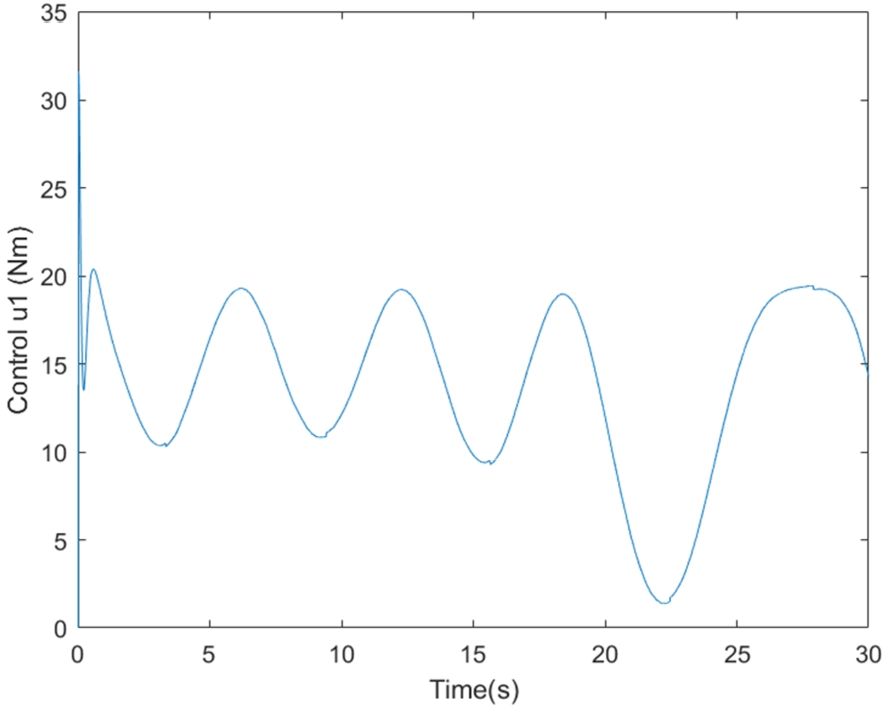
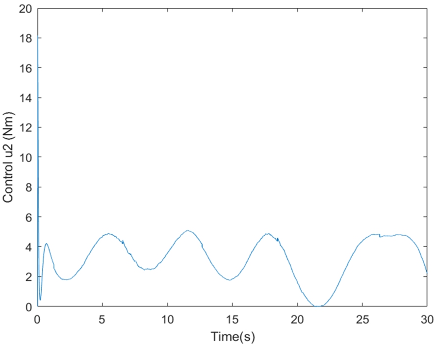
By examining Figs. 1, it can be observed that the position tracking for links 1 represented by dashed line (blue) using the control approach proposed ONNSMC follows perfectly the desired trajectory represented by solid line (red), however, the gap between the position tracking using SMC represented by dot line (black) and the desired trajectory is very significant. Besides, the Figs. 2 represent the control torque signals of the links 1, and it is smooth without any oscillation behaviours even when there are significant uncertainties. In Figs. 3, We can see that the ONNSMC position of link 2 matches closely the reference signals and quickly, however the SMC result position converge to the desired trajectory with meaningful distance. Moreover, Figs. 4 demonstrate that the control torque signals of link 2 is smooth and do not exhibit any oscillatory behavior too.

Fig. 1.

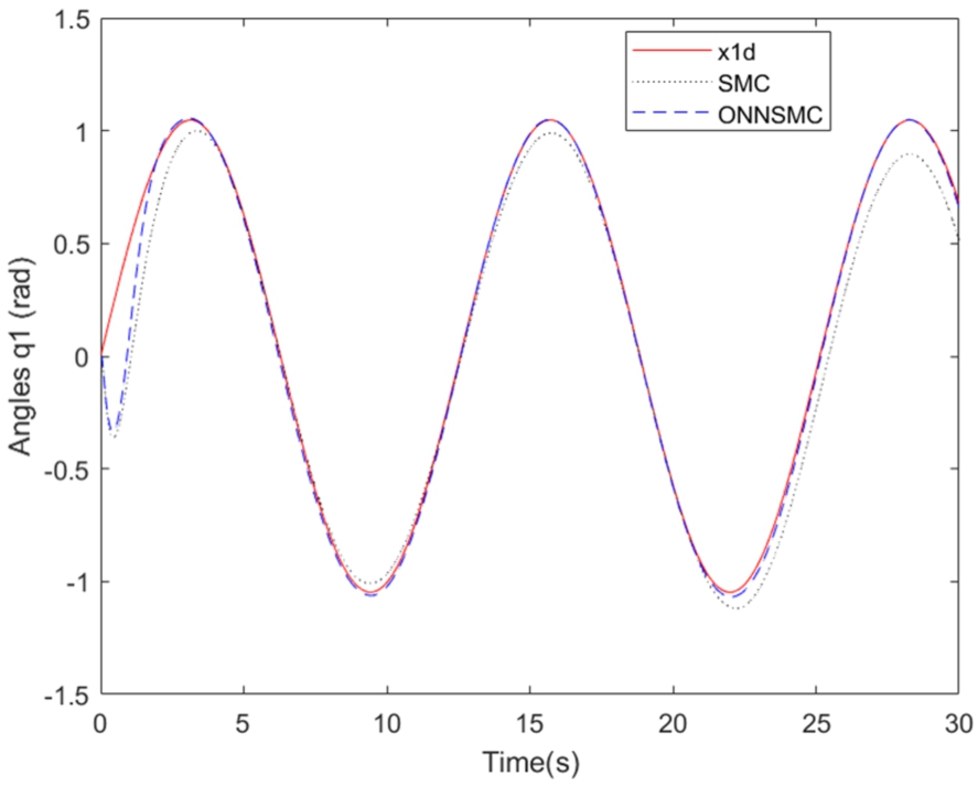
Angles responses x1=q1 using: the proposed ONNSMC, SMC and desired trajectory.

Fig. 2.

The control torque signals τ1 using the proposed ONNSMC.

4.Conclusion

This research paper proposes a novel method for robust optimal reference tracking in two-link robot manipulators by combining traditional sliding mode control with neural networks. Utilizing the neural network involves making an estimation of the nonlinear model function that is not known, and its parameters are adapted through the online BP learning algorithm to provide a better description of the plant. This allows for the use of a lower switching gain, even in the presence of large uncertainties. The ACO algorithm is used to optimize the learning rate of the BP algorithm for faster convergence. Simulation results demonstrate the effectiveness of the proposed method in tracking the reference trajectory without any oscillatory behavior. Future research may explore more efficient optimization methods for the sliding additive control gain. The speed of convergence in terms of the tracking performance is depicted in Figs 1 and 3, that represent the position tracking for link 1 and link 2. The corresponding control torque signals in Figs 2 and 4 are smooth and free of oscillatory behavior.

Fig. 3.

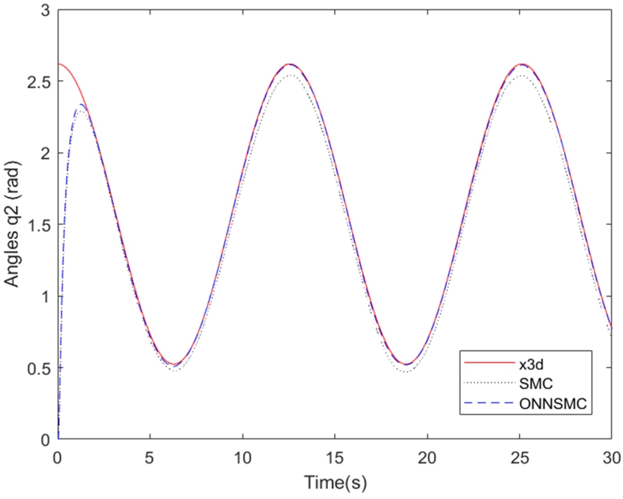
Angles responses x3=q2 using: the proposed ONNSMC, SMC and desired trajectory.

Fig. 4.

The control torque signals τ1 using the proposed ONNSMC.

Conflict of interest

None to report.

References

[1]	F.Z. Baghli, L. El Bakkali and Y. Lakhal, Optimization of arm manipulator trajectory planning in the presence of obstacles by ant colony algorithm, Procedia Engineering 181: ((2017) ), 560–567. doi:10.1016/j.proeng.2017.02.434.
[2]	C.Z. Cao, F.Q. Wang and Q.L. Cao, Neural network-based terminal sliding mode applied to position/force adaptive control for constrained robotic manipulators, Adv Mech Eng 10: (6) ((2018) ), 1–8. doi:10.1177/1687814018781288.
[3]	M. Dorigo, Optimization learning and natural algorithms, PhD thesis, Dipartimento di Elettronica, Politecnico di Milano, Milan, Italy, 1992.
[4]	M. Dorigo, V. Maniezzo and A. Colorni, THE ant system: Optimization by a colony of cooperating agents, IEEE Transactions on Systems, Man, and, Cybernetics Part B: Cybernetics ((1996) ), 29–41.
[5]	L. Fu, Neural Networks in Computer Intelligence, McGraw-Hill, New York, (1995) .
[6]	E.-H. Guechi, S. Bouzoualegh, Y. Zennir and S. Blažič, MPC control and LQ optimal control of a two-link robot arm: A comparative study, Machines 6: (3) ((2018) ). doi:10.3390/machines6030037.
[7]	M.A. Hussain and P.Y. Ho, Adaptive sliding mode control with neural network based hybrid models, Journal of Process Control 14: ((2004) ), 157–176. doi:10.1016/S0959-1524(03)00031-3.
[8]	Internal representations by error propagation, Parallel distributed processing, Vol. 1, MIT Press, Cambridge, 1986.
[9]	P.X. Liu, M.J. Zuo and M.Q.H. Meng, Using neural network function approximation for optimal design of continuous-state parallel-series systems, Computers and Operations Research 30: ((2003) ), 339–352. doi:10.1016/S0305-0548(01)00100-9.
[10]	F. Loucif, S. Kechida and A. Sebbagh, Whale optimizer algorithm to tune PID controller for the trajectory tracking control of robot manipulator, Journal of the Brazilian Society of Mechanical Sciences and Engineering ((2020) ). doi:10.1007/s40430-019-2074-32074.
[11]	S. Massou and I. Boumhidi, Optimal neural network-based sliding mode adaptive control for two-link robot, International Journal of Systems, Control and Communications 8: (3) ((2017) ), 204–216. doi:10.1504/IJSCC.2017.085498.
[12]	H.D. Patino, R. Carelli and B.R. Kuchen, Neural networks for advanced control of robot manipulators, IEEE Transactions on Neural Networks 13: ((2002) ), 343–354. doi:10.1109/72.991420.
[13]	H. Rahimi Nohooji, Constrained neural adaptive PID control for robot manipulators, Journal of the Franklin Institute 357: ((2020) ), 3907–3923. doi:10.1016/j.jfranklin.2019.12.042.
[14]	H.J. Rong, J.T. Wei, J.M. Bai, G.S. Zhao and Y.Q. Liang, Adaptive Neural Control for a Class of MIMO Nonlinear Systems with Extreme Learning Machine, Elsevier Neuro Computing, (2015) , pp. 405–414.
[15]	H.J. Rong, J.T. Wei, J.M. Bai, G.S. Zhao and Y.Q. Liang, Adaptive neural control for a class of MIMO nonlinear systems with extreme learning machine, Neurocomputing 149: ((2015) ), 405–414. doi:10.1016/j.neucom.2014.01.066.
[16]	S. Sefreti, J. Boumhidi, R. Naoual and I. Boumhidi, Adaptive neural network sliding mode control for electrically-driven robot manipulators, Control Engineering and Applied Informatics 14: ((2012) ), 27–32.
[17]	H. Shi, Y.B.Y.B. Liang and Z.H. Liu, An approach to the dynamic modeling and sliding mode control of the constrained robot, Adv Mech Eng 9: (2) ((2017) ), 1–10.
[18]	J.J. Slotine, Sliding controller design for non-linear systems, International Journal of Control 40: ((1984) ), 421–434. doi:10.1080/00207178408933284.
[19]	J.J. Slotine and S.S. Sastry, Tracking control of nonlinear systems using sliding surfaces with applications to robot manipulators, International Journal of Control 39: ((1983) ), 465–492. doi:10.1080/00207178308933088.
[20]	V.I. Utkin, Sliding Modes in Control Optimization, Springer-Verlag, (1992) .
[21]	M. Van, X.P. Do and M. Mavrovouniotis, Self-tuning fuzzy PID-nonsingular fast terminal sliding mode control for robust fault tolerant control of robot manipulators, ISA Transactions ((2019) ). doi:10.1016/j.isatra.2019.06.017.
[22]	R.D. Xi, X. Xiao, T.N. Ma and Z.X. Yang, Adaptive sliding mode disturbance observer based robust control for robot manipulators towards assembly assistance, IEEE Robotics and Automation Letters 7: (3) ((2022) ), 6139–6146. doi:10.1109/LRA.2022.3164448.
[23]	Y. Xiuxing, L. Pan and C. Shibo, Robust adaptive fuzzy sliding mode trajectory tracking control for serial robotic manipulators, Robotics and Computer-Integrated Manufacturing 72: ((2021) ), 101884. doi:10.1016/j.rcim.2019.101884.
[24]	A.M. Zanchettin and P. Rocco, Motion planning for robotic manipulators using robust constrained control, Control Eng. Pract. 59: ((2017) ), 127–136.
[25]	S. Zhang, Y.T. Dong and Y.C. Ouyang, Adaptive neural control for robotic manipulators with output constraints and uncertainties, IEEE T Neur Net Lear 29: (11) ((2018) ), 5554–5564.