
Multi-dimensional T-S dynamic fault tree analysis method involving failure correlation
Abstract
The lack of effective failure correlation analysis is one main reason for the gap between the reliability models and the actual complex systems with mixed static and dynamic characteristics. Takagi and Sugeno (T-S) dynamic fault tree is one powerful tool to analyze the static and dynamic failure logic relationship but it assumes the failure probability of the event is independent. Therefore, this paper proposes a multi-dimensional T-S dynamic fault tree analysis method involving failure correlation. The method integrates the failure probability distribution function of basic events with multi-factors and the multi-dimensional copula function, and the important measure of this method is also deduced. The reliability model expression for systems with failure correlations, both in series and in parallel, is discussed and verified. Compare the proposed method with the assumption that the probability of a failure event is independent. This method solves the problem of a large error when ignoring the failure correlation between parts and the degree of the correlation between variables can be characterized. The reliability analysis can be conducted on complex systems affected both by multi-factors and failure correlations. The proposed method is applied to the reliability analysis of a hydraulic height adjustment system and the correctness and superiority of the method are verified.
1Introduction
As modern engineering systems become larger and more complex, and the level of system integration becomes higher, it is crucial to consider various system characteristics to ensure their reliability, which poses a huge challenge to system reliability analysis and evaluation. The system characteristics to be considered mainly include the following aspects: 1) Due to the complexity and diversity of engineering system structure and fault types, the fault evolution process exhibits mixed static and dynamic failure behavior. 2) The occurrence of system failures is often influenced by multi-factors due to the operating mechanism and working environment of the system. 3) The coupling relation of system structure and function makes the system and its components have multimode failure and failure correlation. Several traditional methods have been researched and proven to be powerful tools for analyzing and evaluating system reliability, including Reliability Block Diagram (RBD) [10], Fault Tree Analysis (FTA) [13, 29], Binary Decision Diagram (BDD) [5, 18], Markov chains [1, 24], Bayesian Network (BN) [2], etc. These traditional methods have certain advantages in terms of modeling, execution, and computational efficiency, but also have significant limitations: 1) The RBD is usually based on the static model of the system and cannot consider the effect of dynamic factors on system reliability. 2) Static fault tree analysis has been developed into Dugan dynamic Fault tree analysis (DFTA) that can capture dynamic failure behavior, but it can only perform qualitative analysis and require the assistance of Markov chains or Monte Carlo methods for quantitative calculations. 3) While Markov chains offer a solution to dynamic behavior problems, it is limited by its inability to handle failure behaviors that follow non-exponential distributions. Additionally, in dealing with complex systems, the challenge of exponential growth in state space arises. 4) BDD is a useful tool to evaluate the impact of various factors on decision outcomes. However, its applicability is limited to simple and unambiguous problems. It has proven to be less effective in addressing complex and fuzzy problems, and the modeling process is relatively complex. 5) The BN requires probability calculation and inference during inference, which may require more computing resources and time. Especially in cases where the network is large or has complex structures, the computational complexity will further increase. Traditional analysis methods have not fully considered the effect of mixed static and dynamic failure behavior, multi-factor influencing characteristics and failure correlation on system reliability analysis. With the emergence of the above problems, their limitations are becoming increasingly apparent.
The Takagi-Sugeno dynamic Fault tree analysis (T-S DFTA) method proposed by scholars Yao et al. [4] can describe both static and dynamic failure behavior. It developed after TS-FTA [16], a method can only describe static failure behavior. It overcomes the shortcoming that the DFTA [19] method can only qualitatively analyze. T-S dynamic gates and their event description rules can infinitely approximate the failure behavior of real systems and can describe any form of static and dynamic failure behavior. Furthermore, Yao et al. [3] proposed a continuous-time T-S DFTA method, which is capable of solving the calculation error problem of discrete-time T-S DFTA and indicating the changing trend of system failure probability. Taking the tape winding hydraulic system as an example, Sun et al. [17] applied the continuous-time T-S DFTA algorithm to the quantitative analysis of dynamic system reliability.
In addition to being dynamic, actual systems are also affected by multi-factors. Considering the effect of a wide variety of factors on the system fault probability, Cui and Li [27] proposed a state absorption method and a state recurrence method in accordance with the Space Fault Tree (SFT) to study the logical relationship between reliability and factors. Further considering the effect of multi-factors and taking the electrical system as the research object, the failure probability distribution of the components and the system under the two factors (including time and temperature), as well as the probability importance and criticality importance of the components were obtained [26]. Chen et al. [7] proposed a continuous-time multi-dimensional T-S DFTA and applied it to the reliability analysis of the hydraulic system of concrete pump trucks. Although the above method enhances the description ability of the fault tree and other methods under multi-factors, the failure correlation between the components in the system is not considered.
In the actual system, a wide variety of components have a certain failure correlation due to mutual cooperation. The reliability analysis results will significantly deviate from the actual situation if only the failure independence between components is considered. Thus, the effect of failure correlation problems should be considered. Tang et al. [20] proposed a novel theoretical method for reliability calculation with failure correlation in mechanical systems. The static and dynamic calculation models in accordance with copulas theory were built, and the problem of determining the correlation degree was solved. On that basis, the precision was ensured, and the calculation was simplified significantly. Safaei et al. [12] used a copula to model the dependency structure of components and studied the aging replacement policy for repairable series and parallel systems with n dependent components. Ding et al. [11] developed a reliability analysis method based on Copula Bayesian Network (CBN). The correlation between a wide variety of subsystems and components was considered, and the difficulty of modeling and assessment was overcome. Mahmoudi et al. [8] built a reliability analysis model for weighted-k-out-of-n systems with failure correlation using the copula function. Saberzadeh et al. [30] considered a complex system composed of n independent elements used the copula function to model the dependency between components, and studied the reliability of the system under the degradation performance. These methods mainly focus on solving the problem of failure correlation with copula functions. It needs to be emphasized that there is a lack of research on system reliability analysis when considering the multiple failure modes of components under the effect of multi-factors, as well as the mixed static and dynamic failure behavior and failure correlation.
In this paper, the multi-dimensional T-S dynamic fault tree analysis method involving failure correlation is proposed, in which the failure correlation model is incorporated into the multi-dimensional T-S DFTA model. Then a typical application case is taken as the reliability analysis of a hydraulic transmission system. Hydraulic transmission is developing toward high precision and complexity, so its reliability is affected by multi-dimensional factors other than time, and it has dynamic dependency between components.
The remainder of this paper is organized as follows. Section 2 introduces the multi-dimensional T-S DFTA method. Section 3 is devoted to the failure correlation reliability analysis method. Section 4 provides the multi-dimensional T-S DFTA method for correlation failure. Section 5 presents an example analysis of the hydraulic system to verify the feasibility of the proposed method. Finally, Section 6 concludes the paper.
2Multi-dimensional T-S DFTA method
2.1T-S dynamic gates and their event sequence description rules
The T-S model comprises a series of IF-THEN rules, which can accurately describe nonlinear systems by using a series of local linear subsystems combined with membership functions. T-S dynamic gates and their event sequence description rules can approximate the failure behavior of the real system infinitely and describe any static and dynamic failure behaviors. The T-S dynamic fault tree model is shown in Fig. 1. xi (i = 1, 2, … , n) represents the basic event, and y represents the top event, then G1 represents the T-S dynamic gate.
Fig. 1
T-S dynamic fault tree.
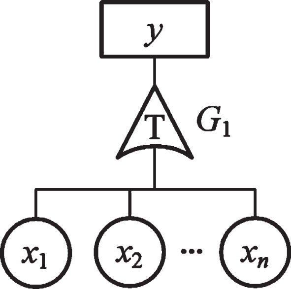
The event sequence description rules include input rules and output rules. The input rules are adopted to describe the fault sequence of basic events x1∼xn, which is expressed by the sequence rule O(l). The output rule describes the failure time of the top event y when the basic event xi fails in a certain sequence. Table 1 lists the event sequence description rules.
Table 1
Event sequence description rules of G1 gate
| Rule | x1 | x2 | ⋯ | xn | O(l) | y |
| 1 | 1 | 2 | ⋯ | n | O(1) | δ(1)(ty) |
| 2 | 1 | 3 | ⋯ | n | O(2) | δ(2)(ty) |
| ⋮ | ⋮ | ⋮ | ⋮ | ⋮ | ⋮ | ⋮ |
| l | o(t1) | o(t2) | ⋯ | o(tn) | O(l) | δ(l)(ty) |
| ⋮ | ⋮ | ⋮ | ⋮ | ⋮ | ⋮ | ⋮ |
| r | n | n-1 | ⋯ | 1 | O(r) | δ(r)(ty) |
In the input rules, the natural numbers o(t1)∼o(tn) are adopted to express the failure occurrence sequence of basic events x1∼xn. The failure occurrence time of the basic events with small values is earlier than that of the basic events with high values.
Boudali [15] employed the unit-step function and impulse function in the continuous-time BN method to describe the dependencies of a complex dynamic system. In accordance with the above idea, the sequence rule O(l) is formed by multiplying a set of unit-step functions. According to the properties of the unit-step function u(ti– t j), it is adopted to describe the fault sequence of basic events x1∼xn.
(1)
In the output rules, the impulse function δ (ty– ti) is employed to describe the failure time of the top event y.
(2)
Rule 1 in Table 1 serves as an example to interpret rules, i.e., basic events x1 to xn are executed according to 1, 2, … , n, and then o(t1) = 1, o(t2) = 2, … , o(tn) = n. The sequence rule O (1) is expressed as follows:
(3)
In this case, the output rule is represented by the impulse function δ (1) (ty) of the top event y.
Compared with conventional logic gates expressing static and dynamic relationships, T-S dynamic gates are capable of characterizing any dynamic logic gate relationships, thus reducing the difficulty of fault tree modeling. For static and dynamic failure behaviors which cannot be expressed by existing logic gates, the corresponding event sequence description rules can be set for modeling and analysis based on T-S dynamic gates. In the following, AND gate and compound dynamic gate are taken as examples of the transformation process of each logic gate to the T-S dynamic gate.
(1) AND gate transforms to T-S dynamic gate
AND gate indicates that the top event occurs when all basic events occur. Table 2 lists the event sequence description rules when T-S dynamic gate is adopted to express the logic of AND gate.
Table 2
Event sequence description rules of the T-S dynamic gate transforming from AND gate
| Rule | x1 | x2 | O(l) | y |
| 1 | 1 | 2 | u(t2– t1) | δ(ty– t2) |
| 2 | 2 | 1 | u(t1– t2) | δ(ty– t1) |
(2) Composite dynamic gate transforms to T-S dynamic gate
Besides AND gate, OR gate, priority-AND gate, etc., T-S dynamic gates can describe any logic relations of events through input and output rules which are maybe difficult to describe with existing logic gates.
The cooling and filtering system in a hydraulic system is taken as an example. The basic events x1 and x2 represent the cooler failure and the filter failure, respectively, and the top event y is the cooling and filtering system failure. When the basic event x1 of the cooler fails, the hydraulic oil temperature increases continuously. It is assumed that after a period d, the oil temperature exceeds the allowable maximum oil temperature of the system, resulting in system failure, i.e., y fails at time ti +d which is later than the time x1 fails. In the other situation, the top event y happens when filtering system x2 fails. Subsequently, the event sequence description rules of the composite T-S dynamic gate are listed in Table 3.
Table 3
Event sequence description rule of composite T-S dynamic gate
| Rule | x1 | x2 | O(l) | y |
| 1 | 1 | 2 | u(t2– t1) | δ(ty– (t1 + d)) |
| 2 | 2 | 1 | u(t1– t2) | δ(ty– t2) |
2.2Multi-dimensional T-S DFTA method
The multi-dimensional T-S DFTA method comprises an input rule and an output rule algorithm in which multi-factors are considered.
(1) Input rule algorithm
The input rule algorithm is capable of obtaining the execution possibility of the respective rule in the T-S dynamic gate.
When the basic events xi(i = 1, 2, … , n) are affected by the working time ti and other k factors (h1, h2, … , hk), the rule execution possibility P* (l) , which describes the rule l is expressed as:
(4)
The failure probability density function is written as follows:
(5)
(2) Output rule algorithm
The failure probability density function and the failure probability distribution function of the top event can be obtained by calculating the rule execution possibility and the top event unit impulse function using the output rule algorithm.
The failure probability density function fy(ty, h1, h2, … , hk) of the top event y represents expressed as:
(6)
The failure probability distribution function Fy(ty, h1, h2, … , hk) is obtained by integrating Equation (6) in the factors as follows:
(7)
2.3Verification of multi-dimensional T-S DFTA method
The multi-dimensional T-S DFTA method is compared with the Dugan dynamic fault tree analysis method based on the Markov chain solution.
(1) Dugan dynamic fault tree analysis method based on Markov chain
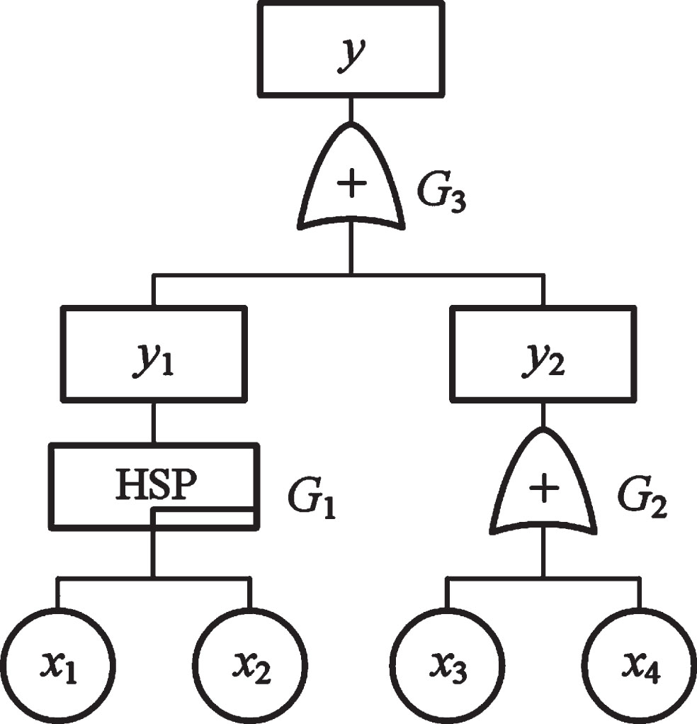
The Dugan dynamic fault tree of a hydraulic system is shown in Fig. 2. G1∼G3 represent hot spare gates, OR gates, OR gates respectively, y is the top event, y1 and y2 are intermediate events, and the failure rates λi of the basic events xi (i = 1, 2, 3, 4) are 2×10⁻⁶/ h, 2×10⁻⁶/ h, 3×10⁻⁶/ h, 6×10⁻⁶/ h, respectively.
Fig. 2
Dugan dynamic fault tree analysis for hydraulic system.
By analyzing the failure principle of the system, the failure path of the system is:
The Markov state transition diagram transformed by the system failure path is shown in Fig. 3.
Fig. 3
Markov state transition diagram.
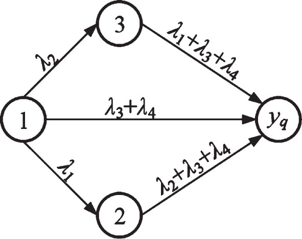
From Fig. 3, the Markov state transition rate matrix D can be obtained as follows:
(8)
According to the Markov differential equation and the state transition rate matrix D, it is obtained that:
(9)
By substituting the task time tM = 10000h, the failure rate of basic events, and the initial value P(0) = [1, 0, 0, 0]T into Equation (9), the failure probability of the system in state Fa can be calculated, and Py(tM) = 0.086427.
(2) Multi-dimensional T-S DFTA method
The Dugan dynamic fault tree of the hydraulic system shown in Fig. 2 is transformed into a multi-dimensional T-S dynamic fault tree shown in Fig. 4.
Fig. 4
Multi-dimensional T-S dynamic fault tree for hydraulic system.
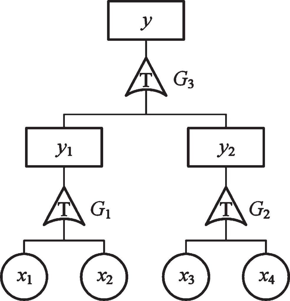
The event sequence description rules of G1∼G3 gates established from the multi-dimensional T-S dynamic fault tree in Fig. 4 are shown in Tables 4–6.
Table 4
Event sequence description rules of G1 gate
| Rule | x1 | x2 | O(l) | y1 |
| 1 | 1 | 2 | u (t2-t1) | δ (ty1-t2) |
Table 5
Event sequence description rules of G2 gate
| Rule | x3 | x4 | O(l) | y2 |
| 1 | 1 | 2 | u (t2-t1) | δ (ty2-t1) |
| 2 | 2 | 1 | u (t1-t2) | δ (ty2-t2) |
Table 6
Event sequence description rules of G3 gate
| Rule | y1 | y2 | O(l) | y |
| 1 | 1 | 2 | u (t2-t1) | δ (ty-t1) |
| 2 | 2 | 1 | u (t1-t2) | δ (ty-t2) |
The failure probability of each component of the hydraulic system obeys the exponential distribution under the influence of the working time t. Through the multi-dimensional T-S DFTA method, from Equations (4) to (7) and Tables 4 to 6, it can be obtained that when the task time tM = 10000h, the failure probability of the top event y is Py(tM) = 0.086427, which is the same as the results calculated by the mothed of Markov chain as above.
The failure probability distribution curve of the top event y with time is shown in Fig. 5.
Fig. 5
Curve of failure probability of top event y changing with time.
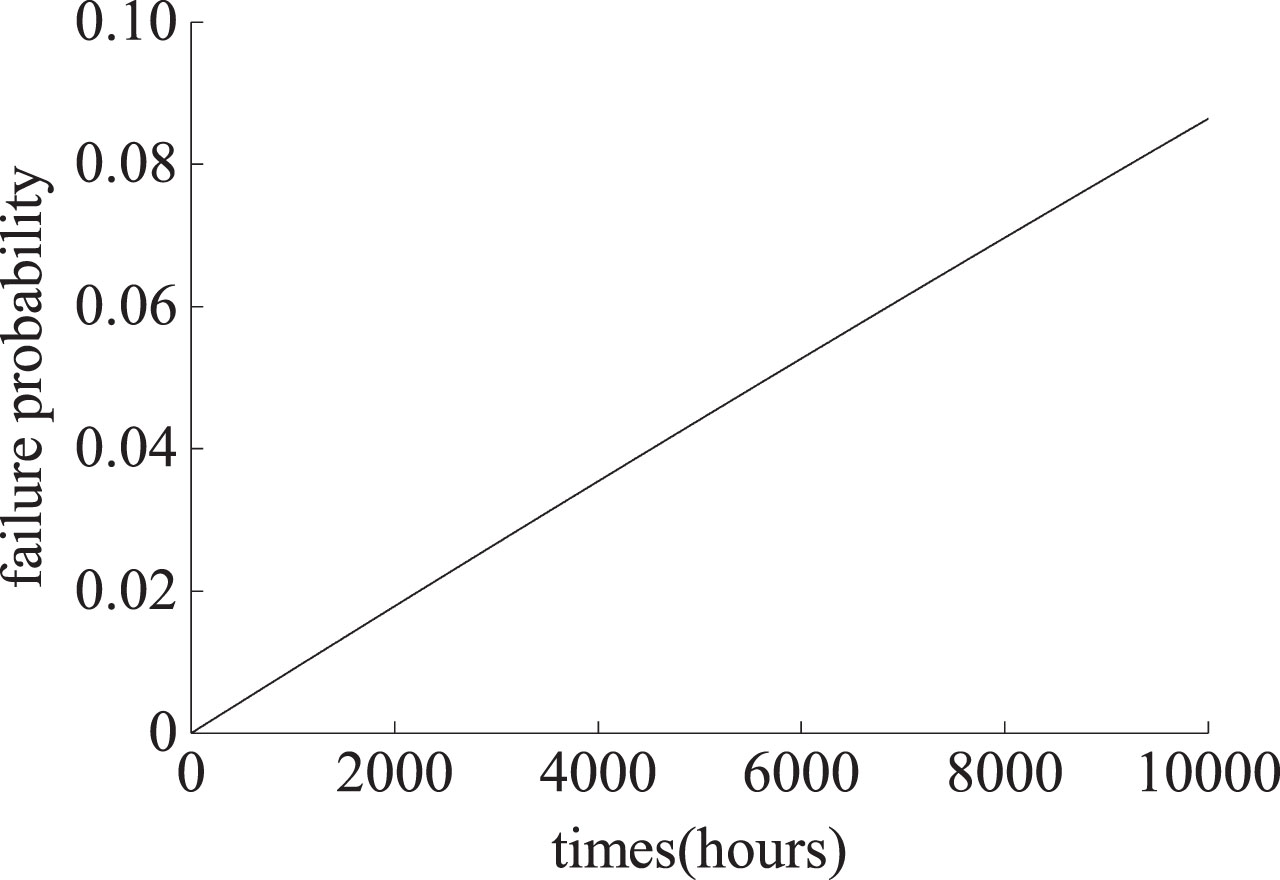
The multi-dimensional T-S dynamic fault tree can show the change curve of the top event failure probability with time. Therefore, the multi-dimensional T-S DFTA method is feasible and superior.
2.4Importance of multi-dimensional T-S DFTA
Importance analysis takes on an essential significance in reliability analysis. The importance ranking of the respective component or subsystem in the system under different conditions can be obtained based on the results of the importance analysis, which is beneficial to find the weak links of the system and enhance its reliability [22].
Probability importance is expressed as the influence degree how basic component reliability changes on system reliability changes. The probability importance of the multi-dimensional T-S dynamic fault tree of basic event xi is written as follows:
(10)
The probability importance of multi-dimensional T-S DFTA refers to the difference of failure probability distribution function of top event y in state yq(q = 1, 2, … , kq) when failure probability distribution function Fi(ti, h1, h2, … , hk) is 1 and 0, respectively.
(11)
3Failure correlation reliability analysis method
Failure correlation is a common phenomenon in mechanical systems or hydraulic systems. Ignoring failure correlation between components will cause deviation in reliability analysis results, so failure correlation should be considered in the reliability analysis process. The copula function is an essential tool to describe the correlation between variables, and it has been extensively employed to solve the problem of failure correlation.
3.1Sklar theorem for n-dimensional copula functions
Let X = (X1, X2, … , Xn) be an n-dimensional random vector, its marginal distribution function is F1(x1), F2(x2), … , Fn(xn), and the joint distribution function is H(x1, x2, … , xn), then there is a unique n-dimensional copula function Cn(u1, u2, … , un), so that for any (x1, x2, … , xn)∈Rn, can be obtained:
(12)
When all the components of an n-dimensional random variable X = (X1, X2, … , Xn) are independent of each other, it can be obtained that:
(13)
3.2Common copula functions
There are some types of common copula functions [9, 21, 25] as shown in Table 7.
Table 7
Two-dimensional Copula function and its tail dependence
| Function Type | C (u, v ; θ) | Tail dependence |
| Gauss |
| Tail symmetry |
| Gumbel | exp(- [(- ln u) 1/θ + (- ln v) 1/θ] θ) , θ ∈ (0, 1] | Right tail correlated |
| Clayton | (u-θ + v-θ-1) -1/θ, θ ∈ (0, ∞) | Left tail correlated |
| Frank |
| Tail symmetry |
3.3Failure correlation reliability model with a series system
For the series system, the failure logic relation is OR gate, i.e., a system failure occurs when any component fails. It is assumed that the series system comprises n components x1, x2, … , xn, and the reliability functions corresponding to the respective component are R1(t), R2(t), … , Rn(t). When the components are independent of each other, the system reliability Ra(t) is expressed as follows:
(14)
Under the complete correlation between components, the reliability Rb(t) of the system is expressed as follows:
(15)
Considering the actual correlation between components in the series system, the actual system reliability R(t) should be within the range of the complete independence and the complete correlation of the respective component, which is expressed as follows:
(16)
The copula function Cn(u1, u2, … , un) is adopted to describe the correlation between the components of the series system, and the reliability of the system Rc(t) is written as [20]:
(17)
The single difference is
Equation (17) suggests that when the series system is consistent with the copula function correlation the fault probability distribution function Fc(t) is expressed as:
(18)
3.4Failure correlation reliability model with a parallel system
In a parallel system, its failure logic relation is AND gate, i.e., the system fails when all components of the system fail. It is assumed that the parallel system consists of n components x1, x2, … , xn and the corresponding reliability function of the respective component is R1(t), R2(t), … , Rn(t). When the correlation between components is not considered, the reliability Ra(t) of the system is written as follows:
(19)
When the complete correlation between components is considered, the reliability Rb(t) of the parallel system is obtained by the component with the greatest reliability, which is expressed as follows:
(20)
The copula function Cn(u1, u2, … , un) is adopted to describe the correlation between the components of the parallel system, and the reliability of the system Rc(t) is written as [20]:
(21)
Equation (21) suggests that when the parallel system is consistent with the copula function correlation, the fault probability distribution function Fc(t) is expressed as follows:
(22)
4Failure correlation reliability analysis method
The multi-dimensional copula function is introduced into the multi-dimensional T-S dynamic fault tree model, so that it can analyze the reliability of failure correlation of complex systems affected by multiple factors. Thus, the failure correlation multi-dimensional T-S DFTA method is proposed.
4.1Multi-dimensional copula function
The system comprises n components xi(i = 1, 2, … , n). When the failure correlation of the respective component is only affected by the working time t, the fault probability distribution function of the respective component is Fi(ti)(i = 1, 2, … , n). The failure probability density function is fi(ti)(i = 1, 2, … , n). Assuming that the joint probability distribution function is F(t1, t2, … , tn), according to Equation (12), there is a unique copula function Cn(u1, u2, … , un) as follows:
(23)
Taking the derivative of the above equation, the joint probability density function f(t1, t2, … , tn) of F(t1, t2, … , tn) is expressed as follows:
(24)
(25)
When the failure correlation of the respective component is affected by t and other k factors (h1, h2, … , hk), the failure probability distribution function of the respective component is Fi(ti, h1, h2, … , hk)(i = 1, 2, … , n), and the failure probability density function is expressed as fi(ti, h1, h2, … , hk)(i = 1, 2, … , n). The joint probability distribution function F(t, h1, h2, … , hk) and the joint probability density function f(t, h1, h2, … , hk) are expressed as follows:
(26)
(27)
4.2Multi-dimensional T-S DFTA with failure correlation
(1) Dynamic gates of failure correlation and their description rules of event sequence
Let the basic event be xi(i = 1, 2, … , n) and the failure time of each event is ti(i = 1, 2, … , n). To distinguish the multi-dimensional T-S DFTA method with failure correlation from that without failure correlation, the top event and its failure time under failure
Fig. 6
T-S dynamic fault tree with failure correlation.
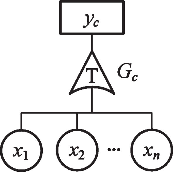
Table 8
Events sequence description rules of Gc gate
| Rule | x1 | x2 | ⋯ | xn | O(l) | yc |
| 1 | 1 | 2 | ⋯ | n | O (1) | δ(1) (tyC) |
| 2 | 1 | 3 | ⋯ | n | O (2) | δ(2) (tyC) |
| ⋮ | ⋮ | ⋮ | ⋮ | ⋮ | ⋮ | ⋮ |
| l | o(t1) | o(t2) | ⋯ | o(tn) | O(l) | δ(l) (tyC) |
| ⋮ | ⋮ | ⋮ | ⋮ | ⋮ | ⋮ | ⋮ |
| r | n | n-1 | ⋯ | 1 | O (r) | δ(r) (tyC) |
(2) Multi-dimensional T-S DFTA with failure correlation
1) Input rule algorithm
When there is failure correlation between the basic events xi(i = 1, 2, … , n), the joint probability density function f(t, h1, h2, … , hk) is adopted to replace the product of the failure probability density functions of each event. Moreover, the rule execution possibility
(28)
When the respective basic event xi(i = 1, 2, … , n) is independent of each other, it yields:
(29)
The result of Equation (29) is consistent with Equation (4), thus suggesting that when the basic event is independent of each other, the rule execution possibility obtained by the copula function is consistent with multi-dimensional T-S DFTA method without failure correlation.
2) Output rule algorithm
Based on the above input rule algorithm, the failure probability density function of the top event yC with failure correlation is expressed as follows:
(30)
By integrating Equation (30) within working time t, the failure probability distribution function of yC with failure correlation is expressed as follows:
(31)
4.3Importance of multi-dimensional T-S DFTA with failure correlation
The probability importance equations of multi-dimensional T-S dynamic fault tree with failure correlation is derived as below.
When the basic event xi(i = 1, 2, … , n) has failure correlation, the probability importance IPrC(xi) with failure correlation is expressed as follows:
(32)
4.4Verification of multi-dimensional T-S DFTA with failure correlation
The series system is taken as an example for verification. It is assumed that a series system comprises components x1 and x2. When the failure of the system is only affected by the working time t, the failure probability distribution function of the two components is denoted as F1(t1) and F2(t2), and the failure probability density function is expressed as f1(t1) and f2(t2). The copula function C(F1(t1), F2(t2)) is adopted to represent the failure correlation of the two components. The multi-dimensional T-S DFTA with failure correlation is employed to solve the failure probability distribution function of the series system.
The T-S dynamic fault tree with failure correlation of the series system is built. Table 9 lists the event sequence description rules of gate Gc.
Table 9
Event sequence description rules of Gc gate
| Rule | x1 | x2 | O(l) | yc |
| 1 | 1 | 2 | u (t2-t1) | δ (tyC-t1) |
| 2 | 2 | 1 | u (t1-t2) | δ (tyC-t2) |
According to the input rule algorithm, the rule execution possibility in Table 9 can be calculated as follows:
(33)
(34)
In accordance with the output rule algorithm, the failure probability density function and failure probability distribution function of the series system are expressed as follows:
(35)
(36)
According to Equation (18), the failure probability distribution function Fc(t) of the series system in compliance with the conventional copula function can be obtained:
(37)
Equations (36) and (37) suggest that the failure probability distribution function solved by the multi-dimensional T-S DFTA with failure correlation is consistent with that solved using the reliability model of the failure correlation series system [14]. As a result, the correctness of the model in solving the reliability problem of the failure correlation series system is verified.
When considering that the failure of the series system is affected by three factors, taking working time t, working temperature T and shock number s as the examples, the failure probability distribution functions of components x1 and x2 are expressed as F1(t1, T1, s1) and F2(t2, T2, s2), respectively. The correlation between components is expressed by copula function C(F1(t1, T1, s1), F2(t2, T2, s2)), and the fault probability distribution function F(t, T, s) of the system is expressed as follows:
(38)
4.5Advantages
The failure correlation multi-dimensional T-S DFTA method can comprehensively consider and analyze multi-factor influence problems and failure correlation problems in the system. The problem of large errors can be solved by considering the system’s static and dynamic characteristics and taking into account the correlation between parts. The results of the reliability analysis are closer to the real situation. It reduces the misjudgment of system failure probability and component importance ranking when considering fault correlation. It has advantages over the multi-dimensional T-S DFTA method without considering failure correlation.
5Case analysis
The shearer has been confirmed as the critical equipment for the fully mechanized mining face in the coal mine. The shearer comprises the cutting department for coal cutting, the transmission system for power transmission, as well as the hydraulic height adjustment system [23]. To be specific, the hydraulic height adjustment system is a vital part of the shearer, which is mainly responsible for adjusting the height of the cutting drum [28]. It is easy to fail in a working environment with high dust, complex force, narrow space and long working hours. Thus, it is necessary to conduct reliability analysis of the hydraulic height adjustment system.
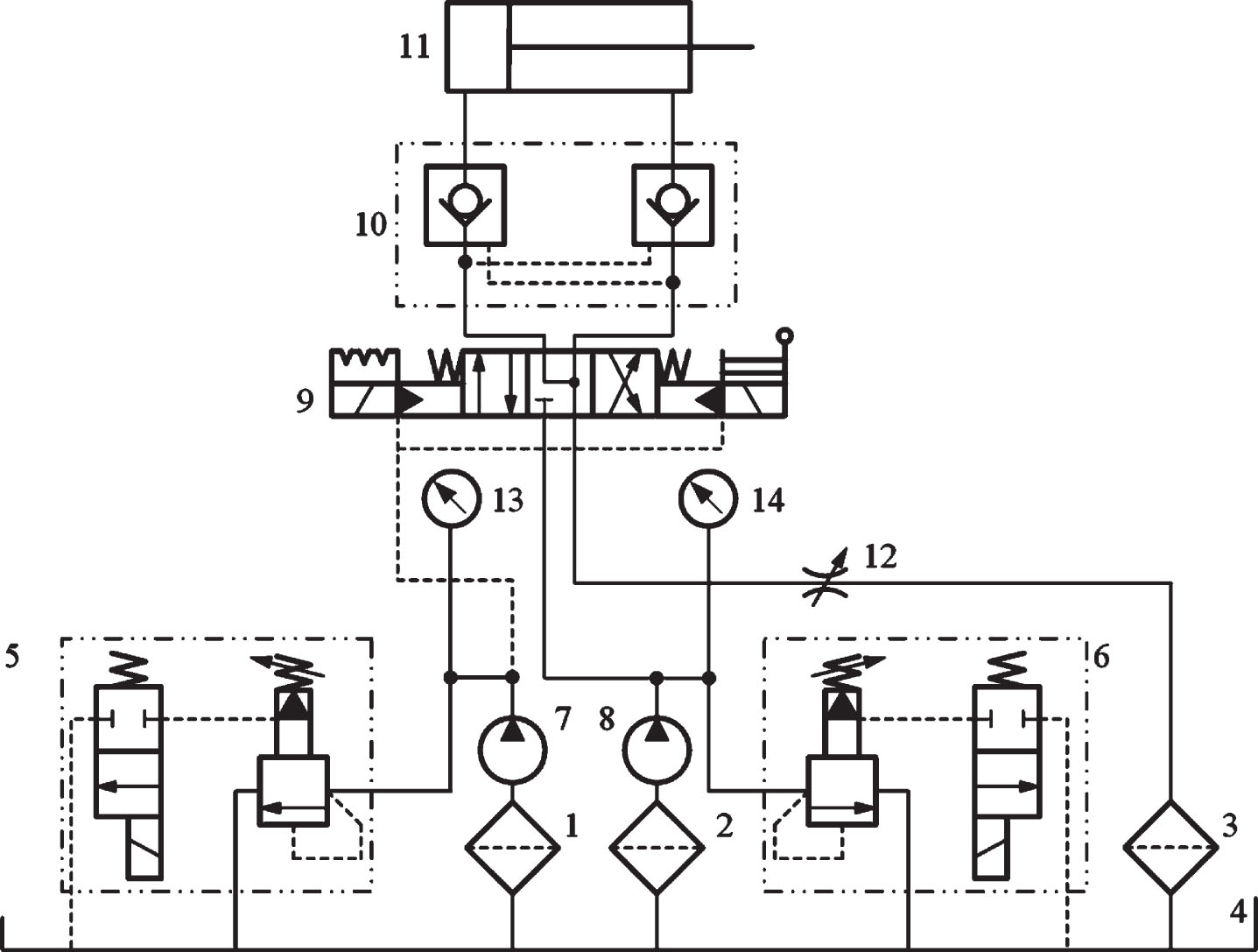
Figure 7 depicts the hydraulic principal diagram of the shearer hydraulic height adjustment system. The externally controlled electro-hydraulic reversing valve controls the action of raising the cylinder, and the low-pressure pump provides externally controlled pressure oil for the electro-hydraulic reversing valve. The electro-hydraulic reversing valve with an emergency handle can be manually reversed by the emergency handle when the electromagnetic pilot valve cannot be changed. The hydraulic lock cooperates with the Y-type neutral function reversing valve, so that the height adjustment oil cylinder can be stopped at any position and can be prevented from moving after stop.
Fig. 7
Principal diagram of hydraulic height adjustment system.
5.1System reliability analysis without failure correlation
(1) Failure probability analysis
Based on the working principle and failure mechanism of the hydraulic height adjustment system of the shearer, the multi-dimensional T-S dynamic fault tree of the hydraulic height adjustment system is built as shown in Fig. 8. G1, G4∼G7 represent the T-S dynamic OR gate, G2 represents the T-S dynamic cold-spare gate, and G3 represents the T-S dynamic priority-AND gate, respectively. x1∼x12 are basic events, and the specific event names and failure rates are shown in Table 10 [6]. y is the top event. y1∼y6 represents intermediate events, and the specific event names are: filter system failure, pilot valve commutation failure, hydraulic oil contamination, Electrohydraulic reversing valve failure, oil supply system failure, and execution system failure.
Fig. 8
Multi-dimensional T-S dynamic fault tree for hydraulic height adjustment system.

Table 10
Name and failure rate of basic event
| Event code | Event name | Failure Rate (×10–6/h) | Event code | Event name | Failure Rate (×10–6/h) |
| x1 | Oil suction filter 1 | 0.3 | x8 | High-pressure pump | 13.5 |
| x2 | Oil suction filter 2 | 0.3 | x9-1 | Solenoid pilot valve of electro-hydraulic reversing valve | 4.5 |
| x3 | Oil return filter | 0.5 | x9-2 | Manual pilot valve of electro-hydraulic reversing valve | 3.5 |
| x4 | Hydraulic oil | 0.5 | x9-3 | Main valve of electro-hydraulic reversing valve | 4.0 |
| x5 | Electromagnetic relief valve 1 | 4.7 | x10 | Hydraulic lock | 1.1 |
| x6 | Electromagnetic relief valve 2 | 4.7 | x11 | Height adjustment cylinder | 5.5 |
| x7 | Low-pressure pump | 9.0 | x12 | Throttle valve | 3.5 |
In the hydraulic height adjustment system, the life of the electromagnetic relief valve and the hydraulic pump is significantly affected by the hydraulic shock. Let the shock obey a Weibull distribution, and its failure probability distribution function is as follows, and its parameters are shown in Table 11.
(39)
Table 11
Weibull parameters of the basic events
| Basic event xi | Component name | Shape parameter m | Characteristic life η/(×106 times) |
| x5, x6 | Electromagnetic relief valve | 4.0521 | 13.0173 |
| x7, x8 | Hydraulic pump | 3.0791 | 1.8992 |
where m is the shape parameter, s is the number of shocks, and η is the characteristic life.
The event sequence description rules for gates G1∼G7 are built, and the G1, G2 and G3 gates are used as an example for description. The event sequence description rules for the G1 gate are shown in Table 12.
Table 12
Event sequence description rules of G1 gate
| Rule | x1 | x2 | x3 | O(l) | y1 |
| 1 | 1 | 2 | 3 | u(t3– t2)u(t2– t1) | δ (ty1-t1) |
| 2 | 1 | 3 | 2 | u(t2– t3)u(t3– t1) | δ (ty1-t1) |
| 3 | 2 | 1 | 3 | u(t3– t1)u(t1– t2) | δ (ty1-t2) |
| 4 | 2 | 3 | 1 | u(t2– t1)u(t1– t3) | δ (ty1-t3) |
| 5 | 3 | 2 | 1 | u(t1– t2)u(t2– t3) | δ (ty1-t3) |
| 6 | 3 | 1 | 2 | u(t1– t3)u(t3– t2) | δ (ty1-t2) |
The event sequence description rules for the G2 gate are shown in Table 13.
Table 13
Event sequence description rules of G2 gate
| Rule | x9-1 | x9-2 | O(l) | y2 |
| 1 | 1 | 2 | u (t9-2-t9-1) | δ (ty2-t9-2) |
The event sequence description rules for the G3 gate are shown in Table 14.
Table 14
Event sequence description rules of G3 gate
| Rule | y1 | x4 | O(l) | y3 |
| 1 | 1 | 2 | u (t4-ty1) | δ (ty3-t4) |
| 2 | 2 | 1 | u (ty1-t4) | 0 |
When the failure probability of the respective component obeying the exponential distribution is only under the effect of the working time t and the task time is tM = 5000h, the failure probability distribution of the top event y can be obtained by the multi-dimensional T-S DFTA method as shown in Fig. 9.
Fig. 9
Failure probability distribution of top event y without failure correlation.
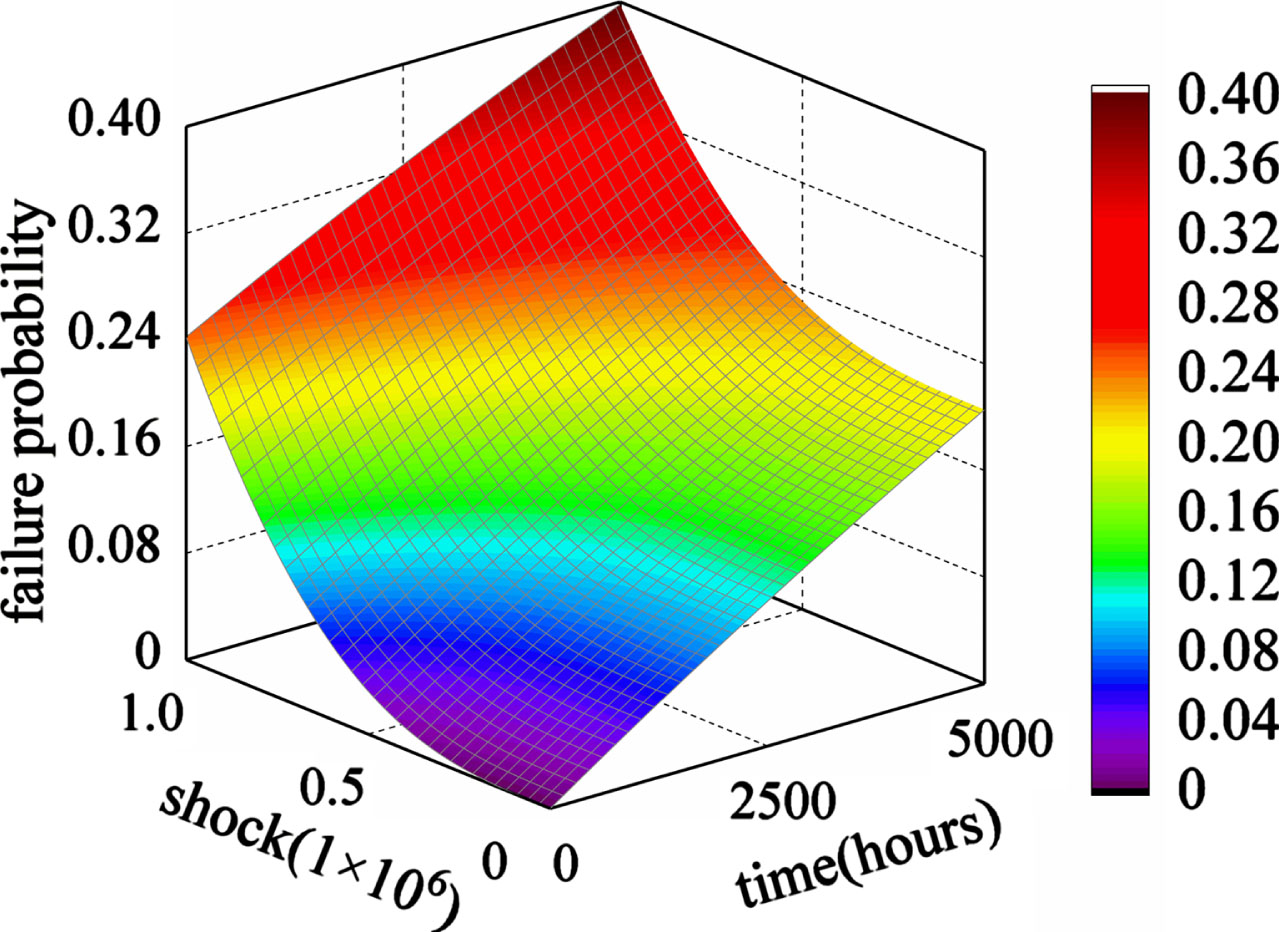
As depicted in Fig. 9, the relationship between the two factors on the top event failure probability of the hydraulic height adjustment system is shown. when the working time t increases from 0 to 5000h, the failure probability value increases from 0 to nearly 0.2 when only the time factor is considered. With the increase of the number of shock s from 0 to 1×10⁶ times, the failure probability value increases from 0 to nearly 0.24 when only shock number factor is considered. When t = 5000h, s = 1×10⁶ times, the failure probability achieves the maximum value of 0.4. It can be seen that compared with only considering the influence of a single factor on the probability of system failure, the multi-dimensional T-S DFTA method considering multiple influencing factors can obtain more comprehensive results when analyzing the reliability of the system.
(2) Probability importance analysis
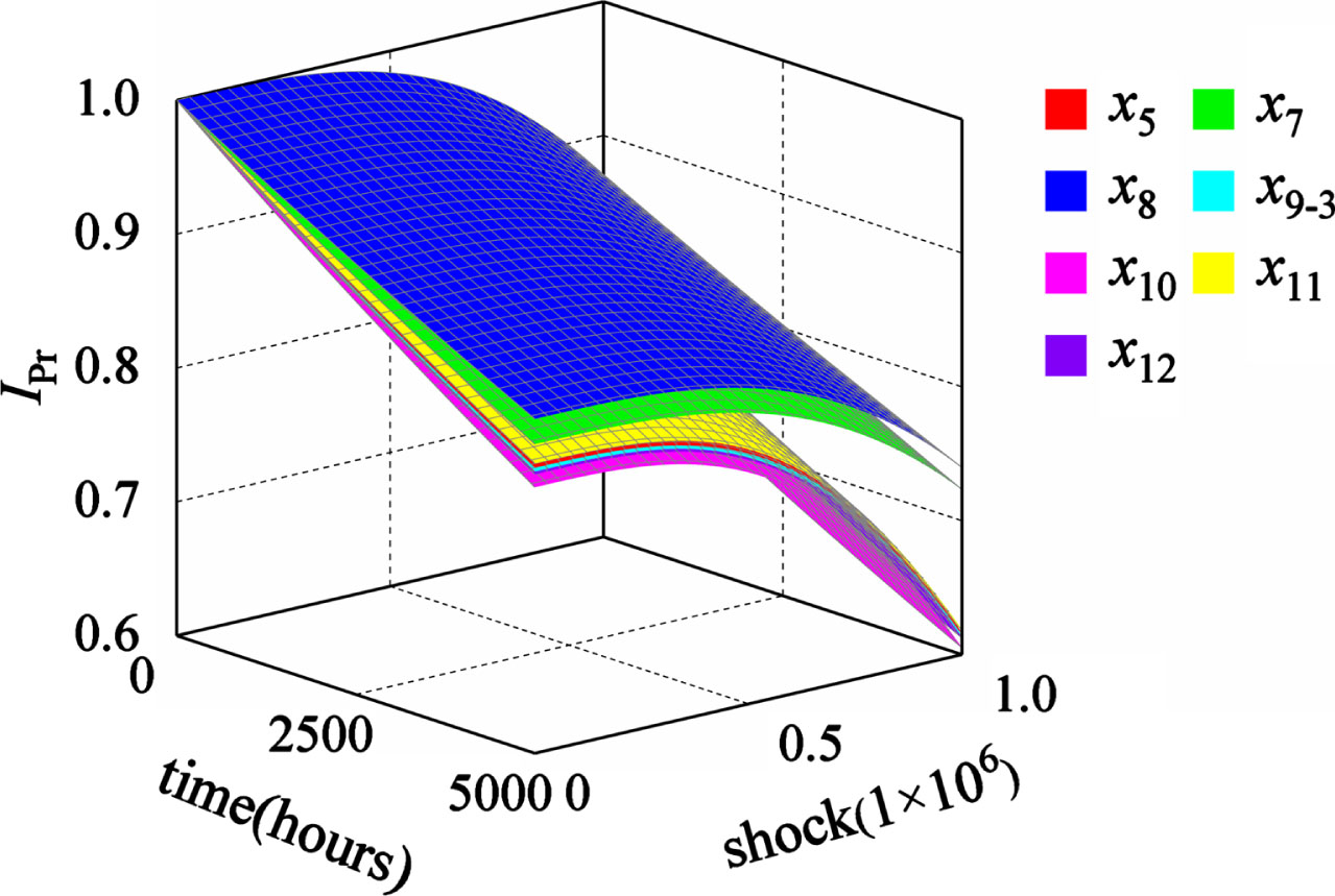
The probability importance of the respective basic event of the hydraulic height adjustment system is expressed in Equation (10), which can be classified into two types in accordance with the different distribution trends and the magnitude. The first type of probability importance involves basic events x1, x2, x3, x4, x9-1 and x9-2, as presented in Fig. 10. The second type of probability importance comprises basic events x5, x6, x7, x8, x9-3, x10, x11 and x12, as illustrated in Fig. 11.
Fig. 10
The first type of probability importance without failure correlation.
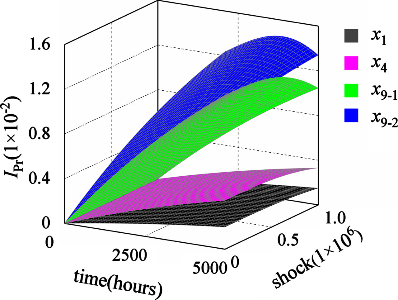
Fig. 11
The second type of probability importance without failure correlation.
In the first type of probability importance, the descending order is x9-2 = x9-1, x4, x3, x1 = x2. The distributions of x1, x2 are the same and both are close to x3, so that x2 and x3 are not drawn in Fig. 10. As depicted in Fig. 10, the probability importance of x1, x4, x9-1 and x9-2 increases with the extension of the working time, whereas x9-1 and x9-2 increase faster than x1 and x4. With the increase of the number of shocks, it shows a distribution trend of first increasing and then decreasing, whereas the trends of x9-1 and x9-2 are more significant than those of x1 and x4.
In the probability importance of the second type of Fig. 11, the descending order is x8, x7, x11, x5, x9-3, x12 and x10. x5 is equivalent to x6.
The comparison between Figs. 10 and 11 suggests that when failure correlation is not involved, the probability importance of the second type is larger than that of the first type. According to the trend of the probability importance of the basic events in Fig. 11 it can be seen that basic events x11, x5, x9-3, x12 and x10 change relatively large and should be focused on.
5.2System reliability analysis with failure correlation
The hydraulic transmission system is dependent on hydraulic oil who circulates in the system as the working medium for transmitting energy. The failure of the hydraulic components will have more correlation when the oil is polluted. Accordingly, the reliability analysis results will be more realistic when the failure correlation between components is considered in the reliability analysis of the hydraulic system.
(1) Failure probability analysis
As depicted in Fig. 12, the multi-dimensional T-S dynamic fault tree copula model of the system is built based on the multi-dimensional T-S dynamic fault tree of the hydraulic height adjustment system and the failure correlation contents of the basic events. x1∼x12 represent the basic events, which are the same hydraulic components as those represented by the multi-dimensional T-S DFTA without considering failure correlation in Section 5.1. Unlike y1∼y6 and G1∼G7 in Section 5.1, yc1∼yc6 denote the failure correlation intermediate events, and Gc1∼Gc7 are failure correlation T-S dynamic gates whose logical relationship between subordinate events is expressed by the corresponding copula function.
Fig. 12
Multi-dimensional T-S dynamic fault tree copula model for hydraulic height adjustment system.
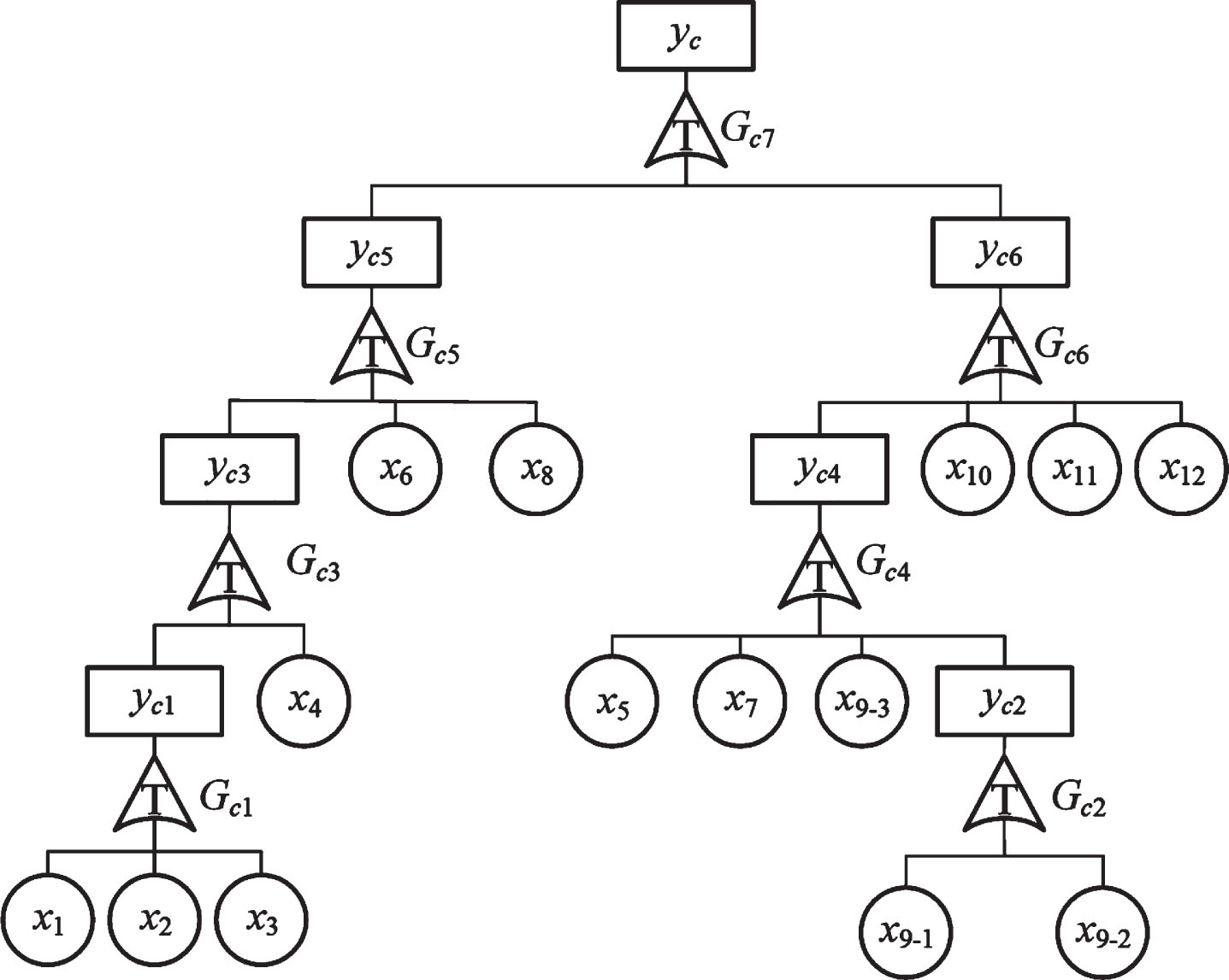
Since the correlation between the life of mechanical parts is generally positive, Gumbel-Copula will be selected as the copula function based on the requirements of model parameter estimation and simple calculation. The failure correlation degree of the subordinate event is changed by changing the correlation coefficient θ of the copula function. The multi-dimensional T-S dynamic fault tree copula model is equivalent to the multi-dimensional T-S dynamic fault tree model when there is no correlation between subordinate events, i.e., when they are entirely independent. The failure correlation between the basic events x5 and x7, x6 and x8, x10, x11 and x12 is considered in the hydraulic height adjustment system. The copula function types and Correlation coefficient θ used by x5 and x7, x6 and x8, x10, x11 and x12 are shown in Table 15.
Table 15
Basic event failure correlation content
| Event code | Copula function | Correlation coefficient θ |
| x5 and x7 | Gumbel Copula | 0.2 |
| x6 and x8 | Gumbel Copula | 0.2 |
| x10, x11 and x12 | Gumbel Copula | 0.3 |
The event sequence description rules for the failure correlation T-S dynamic gates Gc1∼Gc7 are built, and Gc1 is taken as an example for illustration, as shown in Table 16.
Table 16
Event sequence description rules of gate Gc1
| Rule | x1 | x2 | x3 | O(l) | y1 |
| 1 | 1 | 2 | 3 | u(t3– t2)u(t2– t1) | δ (tyc1-t1) |
| 2 | 1 | 3 | 2 | u(t2– t3)u(t3– t1) | δ (tyc1-t1) |
| 3 | 2 | 1 | 3 | u(t3– t1)u(t1– t2) | δ (tyc1-t2) |
| 4 | 2 | 3 | 1 | u(t2– t1)u(t1– t3) | δ (tyc1-t3) |
| 5 | 3 | 2 | 1 | u(t1– t2)u(t2– t3) | δ (tyc1-t3) |
| 6 | 3 | 1 | 2 | u(t1– t3)u(t3– t2) | δ (tyc1-t2) |
To be specific, yc1 denotes the upper event under failure correlation, thus suggesting filter system failure. In the multi-dimensional T-S dynamic fault tree, the G1 gate denotes an OR gate, so that the failure correlation T-S dynamic gate Gc1 represents the OR gate with failure correlation.
The fault probability distribution of top event yc under failure correlation is obtained from the multi-dimensional T-S dynamic fault tree copula model, as presented in Fig. 13.
Fig. 13
Failure probability distribution of top event yc with failure correlation.
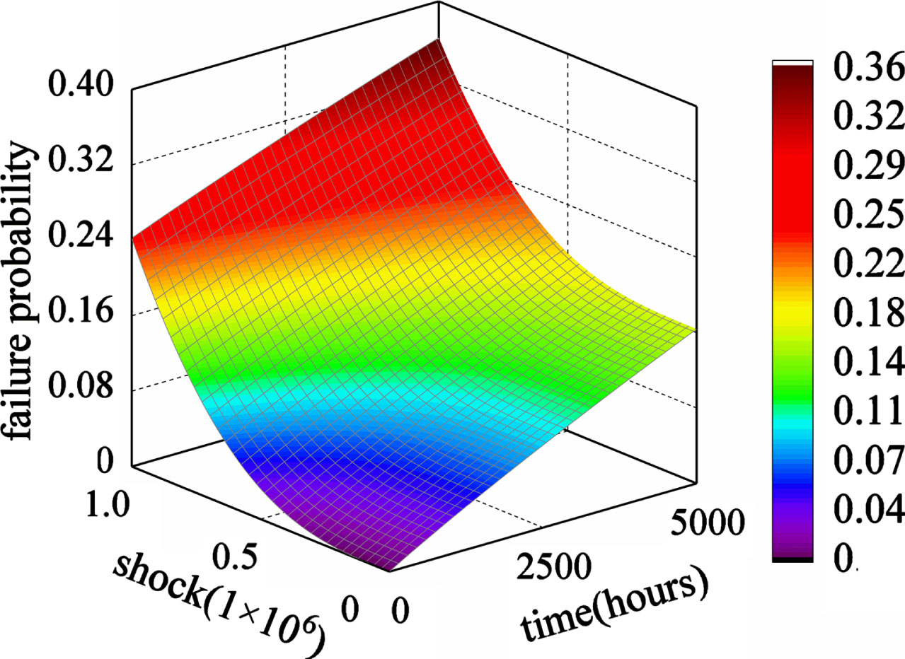
Figure 13 illustrates the changing trend of the failure probability of the top event yc of the hydraulic height adjustment system under t and s. The failure probability of the top event increases with the increase of t and s. Under the effect of the number of shocks s, its upward trend is from slow to fast. Thus, the failure probability of the top event increases with the increase of t and s.
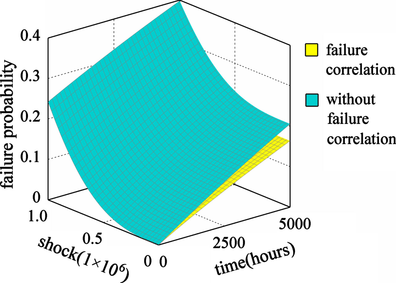
The two failure probability distributions with and without failure correlation are compared to further examine the effect of failure correlation on the overall reliability of the system. As depicted in Fig. 14, the trend of the two changes with the factors is the same, and only the value of the failure probability is different, i.e., the failure probability distribution without failure correlation is slightly more significant than the failure probability distribution with failure correlation. This is because the positive correlation of the basic events is considered in the reliability analysis of failure correlation. Due to the effect of positive correlation between basic events, the survival probability of the respective basic event is greater than that when they are independent of each other, so that the reliability of the system is enhanced, that is, the probability distribution of failures considering failure correlation is smaller than the probability distribution of failures that do not consider failure correlation.
Fig. 14
Comparison of the failure probability distribution.
Only the reliability analysis results at the system level are obtained by solving the system failure probability distribution with failure correlation. The following is a multi-dimensional T-S dynamic fault tree copula importance algorithm for the respective basic event to analyze the probability importance. At the level of basic components, the quantitative reliability analysis of the shearer height adjustment system with failure correlation is carried out.
(2) Probability importance analysis
According to the distribution of the probability importance of the basic events of the hydraulic height adjustment system under failure correlation, the probability importance is divided into two types, and each category contains the same basic events as without considering failure correlation.
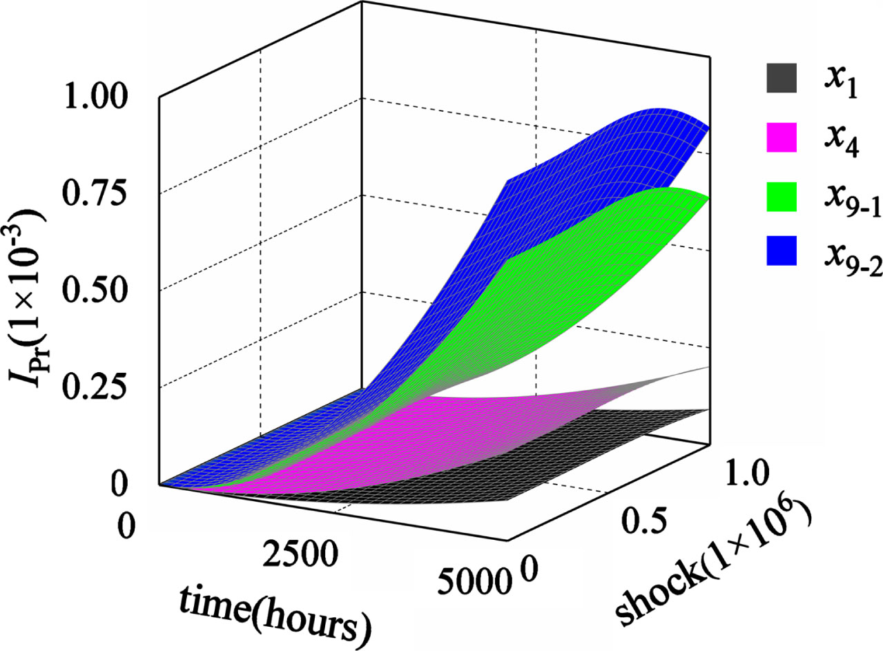
The probability importance of the first type with failure correlation is shown in Fig. 15, and its descending order is x9-2, x9-1, x4, x3 and x1 = x2. To clarify the difference between them, the importance of involving failure correlation is subtracted from that when it is not considered, and the difference of the distribution between the first type of probability importance with and without failure correlation is presented in Fig. 16.
Fig. 15
The first type of probability importance with failure correlation.
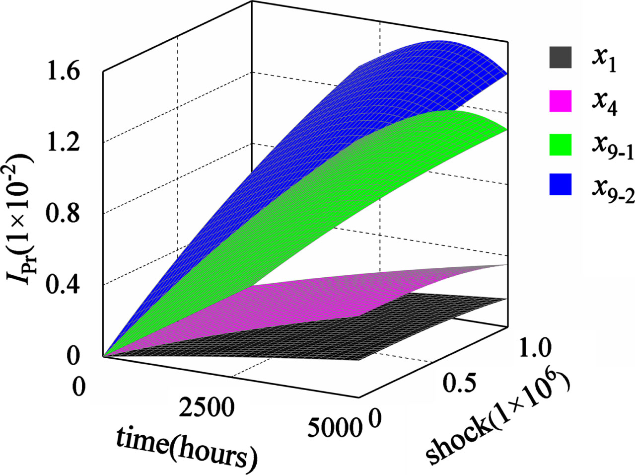
Fig. 16
The difference between the first type of probability importance distributions with and without failure correlation.
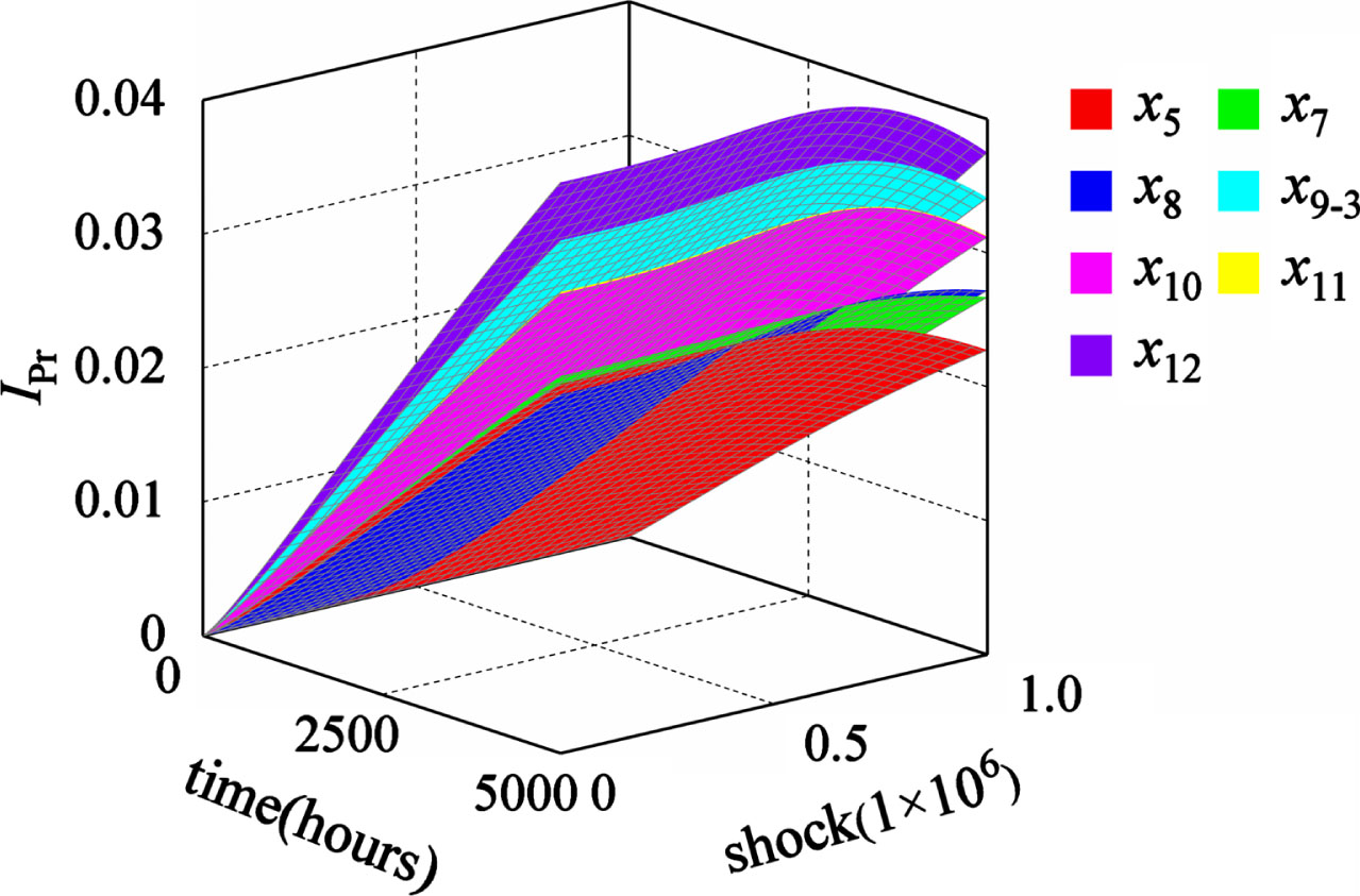
The importance distributions of the second type of probability importance basic events x10 and x5 intersect with failure correlation. x5 is equal to x6. Compared with the case without failure correlation, the importance order of x5, x9-3, x10, x11 and x12 has changed. Fig. 17 illustrates the probability importance distribution of the second type of the basic event under failure correlation. They are sorted from high to low as x8, x7, x9-3, x11, x12, x10 and x5. Fig. 18 presents the difference between the distribution of the second type of probability importance without failure correlation and with failure correlation.
Fig. 17
The second type of probability importance with failure correlation.
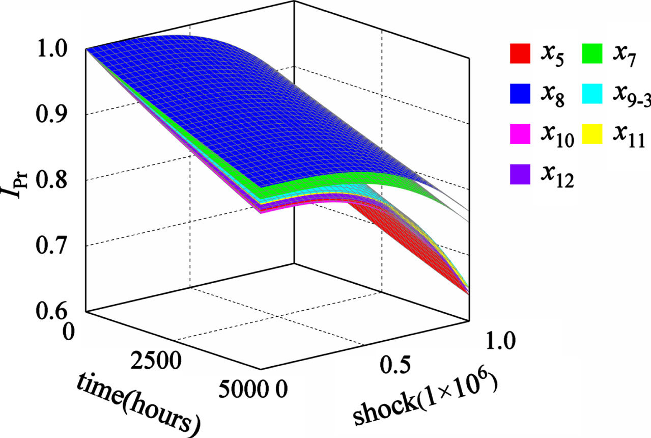
Fig. 18
The difference between the second type probability importance distributions with and without failure correlation.
5.3Result and recommendations
Through the examples studied, it can be seen that compared with not considering the failure correlation, the failure probability of the system top event considering the failure correlation decreases by 0.0368 at t = 5000h, s = 1×10⁶ times. The probability importance of x9-3, x10, and x12 (main valve of electro-hydraulic reversing valve, hydraulic lock, throttle valve) increased by 0.0341, 0.0312, and 0.0375 respectively, which changed significantly compared with that when failure correlation is not considered. In other words, in the actual situation where correlation is widespread, more attention should be paid to x9-3, x10, and x12.
Based on the case analysis presented in this chapter, the findings suggest that neglecting the influence of failure correlation can lead to a misjudgment of the probability of system failure. Such misjudgment can introduce errors into the reliability evaluation process of the system. Additionally, from the ranking results of probability importance, ignoring failure correlation can lead to a misjudgment of important components that have a significant impact on the system. Consequently, this can lead to prioritization errors during maintenance and repair activities. These observations highlight the significance of the proposed method for practical reliability assessment and subsequent maintenance and repair tasks.
6Conclusions
T-S dynamic fault tree is one powerful tool to analyze the static and dynamic failure logic relationship. Based on T-S DFTA, this paper comprehensively studies the reliability analysis of complex systems with mixed static and dynamic characteristics and failure correlation affected by multi-factors. A reliability analysis method of multi-dimensional T-S dynamic fault tree analysis with failure correlation is proposed. Firstly, the T-S DFTA is multi-dimensional processed to enable an analysis of systems affected by multi-factors. Furthermore, the copula function is multi-dimensional processed and integrated into the multi-dimensional T-S DFTA algorithm, which is verified in the series system. Meanwhile, the importance algorithm of multi-dimensional T-S dynamic fault tree with failure correlation is proposed. For the sake of illustration, the method is applied to the hydraulic height adjustment system of a coal mining machine. The system failure probability distribution and basic events importance order of multi-dimensional T-S DFTA are calculated without and with considering failure correlation. The results illustrate that the method is more in line with the actual situation. It lays a theoretical basis for discovering the weak links of the system and enhancing the reliability of the system.
The main attraction of this research lies in its focus on the issue of failure correlation and multi-factors, which expands the framework for reliability assessment and analysis. However, in the present analysis, this paper just discusses the commonly used series and parallel systems, while other types of systems, such as warm-standby and k-out-of-n systems, require further research. In addition, in the future work, this method will catch our focus by considering the optimization of constraints such as cost, weight volume in real systems.
Acknowledgments
This project is supported by the National Natural Science Foundation of China (Grant No. 51975508), Hebei Natural Science Foundation (Grant No. E2021203061).
References
[1] | Peiravi A. , Nourelfath M. and Zanjani M.K. , Redundancy strategies assessment and optimization of k-out-of-n systems based on Markov chains and genetic algorithms, Reliability Engineering & System Safety 221: ((2022) ), 108277. |
[2] | Chuku A.J. , Adumene S. , Orji C.U. et al., Dynamic failure analysis of ship energy systems using an adaptive machine learning formalism, Journal of Computational and Cognitive Engineering ((2022) ), 1–10. |
[3] | Yao C.Y. , Wang C.Y. , Chen D.N. et al., Continuous-time T-S dynamic fault tree analysis method, Journal of Mechanical Engineering 56: (10) ((2020) ), 244–256. |
[4] | Yao C.Y. , Rao L.Q. , Chen D.N. et al., T-S dynamic fault tree analysis method, Journal of Mechanical Engineering 55: (16) ((2019) ), 17–32. |
[5] | Ge D. , Lin M. , Yang Y.H. et al., Quantitative analysis of dynamic fault trees using improved sequential binary decision diagrams, Reliability Engineering & System Safety 142: ((2015) ), 289–299. |
[6] | Chen D.N. , Zhang J.G. , Yao C.Y. et al., Dynamic fault tree analysis of hydraulic heightening system based on DTBN, Machine Tool & Hydraulics 49: (13) ((2021) ), 183–189. |
[7] | Chen D.N. , Xu J.Y. , Yao C.Y. et al., Continuous time multi-dimensional T-S dynamic fault tree analysis method, Chinese Journal of Mechanical Engineering 57: (10) ((2021) ), 231–244. |
[8] | Mahmoudi E. , Meshkat R.S. and Torabi H. , Copula-based reliability for weighted-k-out-of-n systems having randomly chosen components of m different types, IEEE Transactions on Reliability 71: (2) ((2021) ), 630–639. |
[9] | Frees E.W. and Valdez E.A. , Understanding relationships using copulas, North American Actuarial Journal 2: (1) ((1998) ), 1–25. |
[10] | Bistouni F. and Jahanshahi M. , Analyzing the reliability of shuffle-exchange networks using reliability block diagrams, Reliability Engineering & System Safety 132: ((2014) ), 97–106. |
[11] | Ding F. , Wang Y. , Ma G. et al., Correlation reliability assessment of artillery chassis transmission system based on CBN model, Reliability Engineering & System Safety 215: ((2021) ), 107908. |
[12] | Safaei F. , Châtelet E. and Ahmadi J. , Optimal age replacement policy for parallel and series systems with dependent components, Reliability Engineering & System Safety 197: ((2020) ), 106798. |
[13] | Zhang F. , Cheng L. , Gao Y. et al., Fault tree analysis of a hydraulic system based on the interval model using latin hypercube sampling, Journal of Intelligent & Fuzzy Systems 37: (6) ((2019) ), 8345–8355. |
[14] | An H. , Yi H. and He F.K. , Analysis and application of mechanical system reliability model based on copula function, (S1), Polish Maritime Research 23: ((2016) ), 187–191. |
[15] | Boudali H. A temporal Bayesian network reliability modeling and analysis framework, Ph.D. Dissertation, University of Virginia, (2005) . |
[16] | Song H. , Zhang H.Y. and Chan C.W. , Fuzzy fault tree analysis based on T-S model with application to INS/GPS navigation system, Soft Computing 13: (1) ((2009) ), 31–40. |
[17] | Sun H.H. , Xu L.P. , Jiang G.J. et al., Reliability analysis of tape winding hydraulic system based on continuous-time T-S dynamic fault tree, Mathematical Problems in Engineering 2022: ((2022) ), 1–12. |
[18] | Kawahara J. , Sonoda K. , Inoue T. et al., Efficient construction of binary decision diagrams for network reliability with imperfect vertices, Reliability Engineering & System Safety 188: ((2019) ), 142–154. |
[19] | Dugan J.B. , Bavuso S.J. and Boyd M.A. , Fault trees and sequence dependencies, Microelectronics Reliability 31: (5) ((1991) ), 286–293. |
[20] | Tang J.Y. , He P. and Wang Q. , Copulas model for reliability calculation involving failure correlation, Wuhan, China, In 2009 International Conference on Computational Intelligence and Software Engineering ((2009) ), 1–4. |
[21] | Xu L. , Liu Y. and Liu H.B. , Linguistic interval-valued intuitionistic fuzzy copula power aggregation operators for multiattribute group decision making, Journal of Intelligent & Fuzzy Systems 40: (1) ((2021) ), 605–624. |
[22] | He L.P. , Huang H.Z. , Pang Y. et al., Importance identification for fault trees based on possibilistic information measurements, Journal of Intelligent & Fuzzy Systems 25: (4) ((2013) ), 1013–1026. |
[23] | Sun L.Q. , Jiang K. , Zeng Q.L. et al., Influence of drum cutting height on shearer cutting unit vibration by co-simulation method, International Journal of Simulation Modelling 20: (1) ((2021) ), 111–122. |
[24] | Luo P. and Wang X.Y. , Research on the resource allocation algorithm based on forecasting in mobile cloud computing, Journal of Intelligent & Fuzzy Systems 35: (2) ((2018) ), 1315–1324. |
[25] | Nelsen R.B. An introduction to copulas, Springer Series in Statistics, Springer Verlag, (2007) , pp. 17–34. |
[26] | Cui T.J. and Li S.S. , Deep learning of system reliability under multi-factor influence based on space fault tree, Neural Computing and Applications 31: (9) ((2019) ), 4761–4776. |
[27] | Cui T.J. and Li S.S. , Study on the construction and application of discrete space fault tree modified by fuzzy structured element, Cluster Computing 22: (3) ((2019) ), 6563–6577. |
[28] | Li W. , Luo C.M. , Yang H. et al., Memory cutting of adjacent coal seams based on a hidden Markov model, Arabian Journal of Geosciences 7: (12) ((2014) ), 5051–5060. |
[29] | Feng X. , Jiang J.C. and Feng Y.G. , Reliability evaluation of gantry cranes based on fault tree analysis and Bayesian network, Journal of Intelligent & Fuzzy Systems 38: (3) ((2020) ), 3129–3139. |
[30] | Saberzadeh Z. and Razmkhah M. , Reliability of degrading complex systems with two dependent components per element, Reliability Engineering & System Safety 222: ((2022) ), 108398. |


