
Collaborative possibilistic fuzzy clustering based on information bottleneck
Abstract
In fuzzy clustering algorithms, the possibilistic fuzzy clustering algorithm has been widely used in many fields. However, the traditional Euclidean distance cannot measure the similarity between samples well in high-dimensional data. Moreover, if there is an overlap between clusters or a strong correlation between features, clustering accuracy will be easily affected. To overcome the above problems, a collaborative possibilistic fuzzy clustering algorithm based on information bottleneck is proposed in this paper. This algorithm retains the advantages of the original algorithm, on the one hand, using mutual information loss as the similarity measure instead of Euclidean distance, which is conducive to reducing subjective errors caused by arbitrary choices of similarity measures and improving the clustering accuracy; on the other hand, the collaborative idea is introduced into the possibilistic fuzzy clustering based on information bottleneck, which can form an accurate and complete representation of the data organization structure based on make full use of the correlation between different feature subsets for collaborative clustering. To examine the clustering performance of this algorithm, five algorithms were selected for comparison experiments on several datasets. Experimental results show that the proposed algorithm outperforms the comparison algorithms in terms of clustering accuracy and collaborative validity.
1Introduction
Clustering is a typical unsupervised learning technique. If objects in the same clusters are more similar, and ones in different clusters are more dissimilar, the final clustering performance will be better. At present, clustering has been widely used in many fields [1–7] such as data mining, pattern recognition, image segmentation, fuzzy network, bioinformatics, etc. In order to make clustering widely available in more fields, it can be applied to large-scale group decision-making [8, 9]. Existing clustering algorithms mainly include hard clustering [10, 11] and fuzzy clustering [12–14]. The former has only two membership degrees, 0 and 1, that is, each data object is strictly divided into a certain cluster; The membership of the latter can have any values within the interval [0,1], that is, a data object can be classified into multiple clusters with different membership. The representative algorithm of fuzzy clustering is the Fuzzy C-Means (FCM) [15] algorithm, which is famous for its simplicity and rapidity but criticized for its sensitivity to the initial cluster centers and noise data. In order to improve the robustness of FCM, the possibilistic c-means (PCM) clustering algorithm introduced in [16] relaxes the requirement for fuzzy membership normalization, thus obtaining a possibilistic partition, thereby reducing the impact of noise data. However, PCM relies on initialization conditions that may produce clustering overlap. To overcome this shortcoming, membership and typicality are introduced in [17], and constraints the sum of typical values from all data points to one cluster is 1 (
The possibilistic fuzzy c-means (PFCM) algorithm [18] based on the FPCM algorithm, efficiently solved the problem that FPCM is prone to produce small typical values when facing large-scale datasets by relaxing the row sum constraints on typical values, and ensuring the generation of better cluster centers. The PFCM algorithm adds weight coefficients a and b for fuzzy membership and typicality, respectively, but lacks a corresponding calculation method for weight coefficients. The study [19] calculated the parameters through the relative importance of data points in the clustering process and assigned new parameters to the membership and typicality, which is called the weight possibilistic fuzzy c-means (WPFCM) clustering algorithm. Since then, some scholars have improved PFCM by changing the distance measure. The Kernel possibilistic fuzzy c-means (KPFCM) [20] introduces a kernel-based similarity measure in the PFCM to map the input data points into a high-dimensional feature space. KPFCM not only handles linearly indistinguishable problems but also keeps the clustering centers in the observation space, which facilitates the description of the clustering results. In [21], a generalized possibilistic fuzzy c-means (GPFCM) clustering algorithm was proposed by replacing the original European distance with a distance function. The algorithm can effectively suppress noise data and accurately classify edge fuzzy data. Using exponential distance instead of Euclidean distance in PFCM, a possibilistic fuzzy Gath-Geva (PFGG) clustering algorithm based on exponential distance was proposed [22]. In this algorithm, the exponential distance uses the fuzzy covariance matrix and exponential function to automatically adjust the distance measure, which facilitates accurate clustering of clusters with different shapes.
A wide range of similarity measures enrich our choices, but at the same time increase the subjectivity in the selection process. To avoid this subjective error, clustering algorithms based on information bottlenecks have attracted much attention. The information bottleneck theory approach, based on the joint probability distribution between data points and features, uses the information loss generated in the process of sample merging as a measurement standard to perform clustering, and achieves a good clustering effect. At present, many clustering algorithms based on information bottlenecks have been proposed [23–25] and have solved some problems very well. In [23], the bottleneck of bicorrelation multivariate information is introduced into multi-view clustering (MVC), thus solving the problem that MVC only learns the correlation relationship between features or clusters, and solving the problem of unsatisfactory clustering performance. In [24], to cope with a large amount of unlabeled and heterogeneous data, shared view knowledge is transferred to multiple tasks enabling automatic classification of human behavior in unlabeled cross-perspective video collections, which can improve the performance of each task. In [25], used interactive information bottlenecks to deal with high-dimensional co-occurrence data clustering problems, and proposed an interactive information bottleneck for high-dimensional co-occurrence data clustering.
Traditional clustering algorithms assume that different features are independent of each other, thus ignoring the correlation between features, which easily affects clustering accuracy. Collaborative clustering utilizes the collaborative relationship between different feature subsets for clustering, which is conducive to forming a more complete and accurate description of the data organization structure. According to the correlation between different feature subsets, the collaborative fuzzy clustering (CFC) algorithm [26] was proposed, which firstly performs clustering based on independent subsets of the data, and then collaboratively generates the final result by exchanging information on the local partition matrix. The study [27] introduced preprocessing method into collaborative fuzzy clustering, and proposed a collaborative fuzzy clustering data analysis method based on a preprocessing-induced partition matrix. The CFC algorithm has been widely used in many fields [28–30], and has been applied to brain MRI images intensity non-uniformity correction, super-pixel satellite influence on surface coverage, and overseas oil and gas exploration, respectively, and achieved relatively better clustering results.
In order to make full use of the relationship between different feature subsets and further improve clustering accuracy, this paper proposed a novel algorithm named collaborative possibilistic fuzzy clustering based on information bottleneck (ib-CPFCM). This algorithm uses the information bottleneck theory to measure the “distance” between the data points and the cluster centers. This theory takes the mutual information loss generated during merging clusters as the similarity measure, and therefore is conducive to improving the clustering accuracy. Besides the theory, the correlation between different feature subsets is used to perform collaborative clustering, and the corresponding fuzzy membership matrix and typical value matrix are obtained, which is easy to form a more complete description of the dataset.
The rest of this paper is organized as follows: Section 2 briefly introduces the PFCM algorithm, information bottleneck theory, and collaborative clustering algorithm. Section 3 introduces the proposed ib-CPFCM algorithm in detail. Section 4 presents the experimental preparation and experimental results. The final section summarizes this paper and proposes further research directions.
2Related works
In this section, we briefly review the PFCM algorithm, information bottleneck theory, and CFC algorithm. Before that, the variables defined in this paper and their mathematical descriptions are given as Table 1.
Table 1
Variables used in this paper
| Variables | Description |
| C, N | Numbers of clusters, data points |
| M, P | Numbers of feature attributes, feature subsets |
| uij, tij [ii] , vi [ii] | Fuzzy membership, typical values, and cluster centers in the iith feature subset |
|
| Euclidean distance, measure the distance between a data point and a cluster |
| Dib (xj, vi) | Mutual information loss |
| X[ii] | iith feature subset |
| m, w, a, b | User-defined parameters |
| ɛ | Threshold, iterative termination criterion |
| rmax | The maximum number of iterations |
| λ | Lagrange multiplier |
| α[i i, kk] | Collaboration coefficient |
| γi | Conversion factor |
2.1PFCM
The PFCM algorithm not only improves FCM in terms of robustness but also overcomes the clustering coincidence problem of the PCM. Furthermore, by relaxing the row sum constraints on typical values, the problem of generating small typical values with an increasing dataset is solved. The objective function of the PFCM algorithm is designed as follows:
(1)
In Eq. (1), U = [uij] C×N and T = [tij] C×N are the fuzzy membership matrix and typical value matrix, respectively. V = {v1, v2, …, vc} is the cluster center matrix, vi denotes the ith cluster center. N and C are the numbers of data points and clusters. The parameters a and b are constants, m and w are fuzzy weighted parameters, and
(2)
(3)
where K is a constant, and the default value is 1. The objective function of this algorithm is restricted by the following: the fuzzy weighted parameters m, w > 1; the parameters a, b, and γi > 0; the value range of fuzzy membership uij and typical value tij in the interval [0,1], and
(4)
(5)
(6)
2.2Information bottleneck theory
Information bottleneck applies the knowledge of information theory to the clustering process, and the desired clustering is the process of minimizing information loss in the cluster aggregation process. To minimize the mutual information loss in the entire clustering process, the greedy aggregation method is usually adopted, and when merging two clusters, the choice results in the smallest mutual information loss in each step.
d (ci, cj) is used to represent the mutual information loss generated by the cluster ci and cj during the merging process, which is calculated as follows:
(7)
(8)
Many existing pieces of literature have shown [33–37] that, the clustering performance of clustering algorithms using information bottleneck as a similarity measure is obviously better than traditional clustering algorithms, and it can better indicate the correlation between data points and features.
2.3CFC clustering algorithm
The CFC algorithm can utilize the collaboration relationship between different feature subsets for clustering. In this algorithm, the collaboration between feature subsets is established through the connection matrix, as shown in Fig. 1. Given an unlabeled dataset X = {x1, x2, …, xN}, it is divided into P feature subsets Xii = {X1, X2, …, XP}. The objective function in CFC [26] is defined as follows:
(9)
Fig. 1
Collaboration in clustering is represented by interaction matrix between subsets.
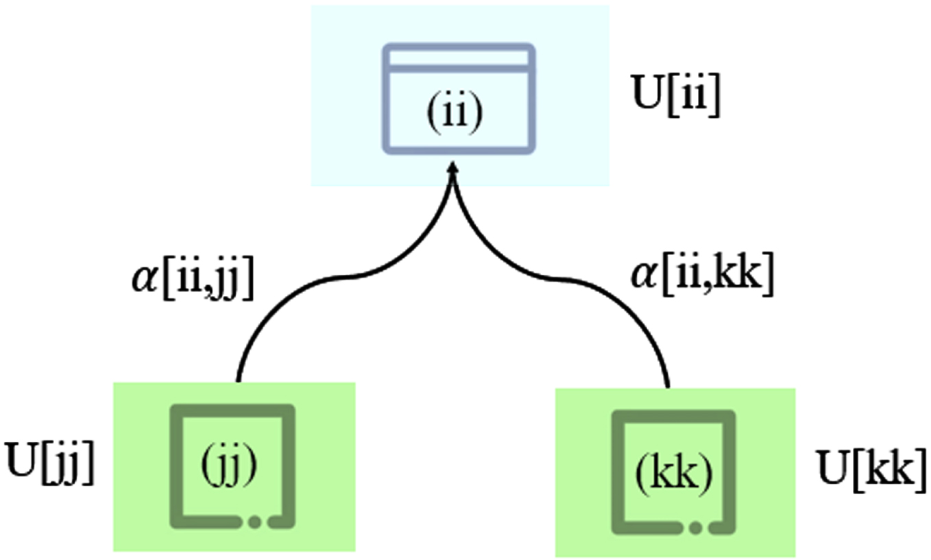
where uij [ii] is the fuzzy membership of the iith feature subset, ii = 1, 2, . . . , P. α[ii, kk] represents the collaboration coefficient and is a non-negative value.
(10)
where M is the number of feature attributes.
3A collaborative possibilistic fuzzy clustering based on information bottleneck
In this paper, based on collaborative clustering and information bottleneck theory, a collaborative possibilistic fuzzy clustering algorithm based on information bottleneck (ib-CPFCM) is proposed. The clustering performance of ib-CPFCM is outstanding because the algorithm uses the mutual information loss generated during merging clusters as a similarity measure, which improves the clustering accuracy in high-dimensional data. ib-CPFCM simultaneously performs collaborative processing of multiple subsets of relevant features, which helps to form an accurate and complete representation of the data organization structure. Given an unlabeled dataset X = {Xii|Xii = X1, X2, …, XP}, the objective function of ib-CPFCM can be expressed as:
(11)
where the first part is the objective function of the possibilistic fuzzy clustering algorithm based on information bottleneck, and the second part is the collaborative relationship among feature subsets. Xii = X1, X2, …, XP represents P feature subsets. U [ii] = uij [ii] C×N and T [ii] = tij [ii] C×N are the fuzzy membership matrix and typical value matrix of the iith dataset, respectively. α[ii, kk] is the collaboration coefficient, and the larger its value indicates the stronger collaboration relationship between two feature subsets. In addition, m and w > 1 are fuzzy weighted parameters, and constants a, b > 0. γi > 0 is the conversion factor, which is defined by
(12)
where xjk [ii] represents the kth attribute value of data point xj in the iith dataset. |c| is the number of data points in each cluster. D (xjk [ii] ∥ hk [ii]) and D (vik [ii] ∥ hk [ii]) are the KL distances, which are estimated using the Monte-Carlo [32] process and the KL distances can be approximated expressed as follows:
(13)
(14)
where M[ii] is the number of feature attributes in the iith dataset, and hk [ii] is calculated as follows:
(15)
The clustering objective of the ib-CPFCM algorithm is to minimize the objective function under the premise of satisfying the constraint conditions. Whereby the Lagrange multiplier method can be used to construct the Lagrange equation as follows:
(16)
Eq. (16) calculates the first order partial derivative of each variable and makes it equal to 0, so that:
(17)
(18)
(19)
(20)
where s = 1, 2, . . . , C. f and j = 1, 2, . . . , N. According to Eqs. (17)–(20), the iterative formulas for the fuzzy membership usf [ii], typicality tsf [ii], and cluster center vsf [ii] of the ib-CPFCM algorithm are deduced as follows:
(21)
(22)
where φsf [ii] and ω [ii] can be represented as:
(23)
(24)
To simplify Eq. (20), Asf [ii], Bs [ii], Csf [ii], and Ds [ii] are introduced, and the calculation method can be represented as:
(25)
(26)
(27)
(28)
Using Eqs. (20), (25), (26), (27), and (28), the cluster center vsf [ii] is calculated as follows:
(29)
The clustering process of this algorithm mainly includes two stages (as shown in Fig. 2):
(1) Possibilistic fuzzy clustering based on information bottleneck
Fig. 2
Two stages of ib-CPFCM clustering algorithm.
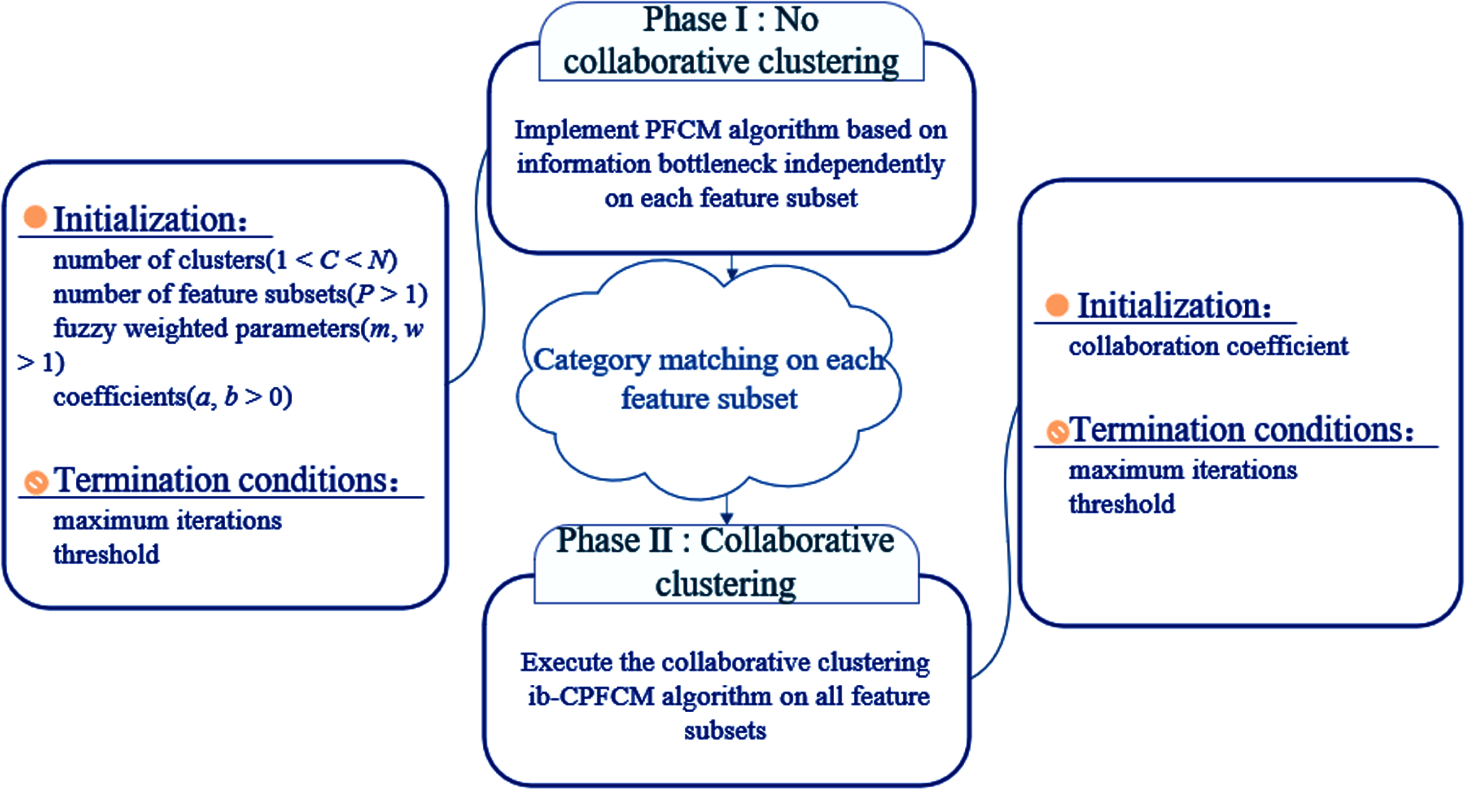
PFCM algorithm based on information bottleneck clusters each feature subset, requiring the same number of data points for each feature subset, and the feature attribute dimensions can be different.
(2) collaborative clustering algorithm
Set the collaboration coefficient α[ii, kk], and perform collaborative optimization on the fuzzy membership matrix, typical value matrix and cluster centers matrix obtained in the first stage.
It should be noted that because each feature subset is an independent cluster, the corresponding cluster in u[ii] and t[ii] is usually inconsistent with the corresponding cluster in u[kk] and t[kk], so it is necessary to perform cluster matching processing on the clustering results of each feature subset.
After the above theoretical analysis, algorithm 1 is the entire process of implementing the ib-CPFCM algorithm:
| Algorithm 1 ib-CPFCM: A Collaborative Possibilistic Fuzzy Clustering Based On Information Bottleneck |
| Input: Dataset X = {X1, X2, …, XP}, |
| C, N, M, P, m, w, a, b, α [ii, kk], ɛ, rmax |
| Output: fuzzy membership matrix U, typical value matrix U[ii], cluster center matrix V[ii] |
| No Collaboration Stage: |
| Each feature subset is clustered under the PFCM algorithm based on information bottleneck |
| Collaboration Stage: |
| Repeat |
| Repeat for each feature subset Xii |
| r = r + 1 |
| For ii = 1: P |
| For f = 1: N |
| For s = 1: C |
| For k = 1: M |
| Calculate Dib (xf, vs) [ii], by using (12) |
| Update usf [ii], by using (21) |
| Update tsf [ii], by using (22) |
| Update vs [ii], by using (29) |
| Until (|SSIGMA-SIGMA|< ɛ) |
| End |
| Return (V, U, T) = (Vr, Ur, Tr) |
4Experiments
In order to evaluate the clustering effectiveness of the ib-CPFCM algorithm, five algorithms were selected for comparison experiments on nine datasets, and their clustering results were compared based on four evaluation indexes.
4.1Experimental preparation
Nine datasets were selected from the UCI machine learning dataset (http://archive.ics.uci.edu/ml/datasets.php) for the comparison experiments, and the specific information of each dataset is shown in Table 2.
Table 2
Features of the dataset
| Dataset | No. of | No. of | No. of |
| objects | features | clusters | |
| Iris | 150 | 4 | 3 |
| Wine | 178 | 13 | 3 |
| Wdbc | 569 | 30 | 2 |
| Ecoli | 336 | 7 | 8 |
| Sonar | 208 | 60 | 2 |
| Dermatology | 366 | 34 | 6 |
| Tae | 151 | 5 | 3 |
| Knowledge | 403 | 5 | 4 |
| Lymphography | 148 | 18 | 4 |
Table 3
Horizontal distribution of datasets
| Dataset | Feature subset |
| Iris | P1{, [1, 2, 3]} |
| P2{[0, 2] , [1, 3]} | |
| P3{[0, 1] , [2, 3]} | |
| Wine | P1{[0, 1, 2, 3, 4, 5, 6, 7, 8, 12] , [7, 8, 9, 10, 11]} |
| P2{[0, 2, 4, 6, 8, 10, 12] , [1, 3, 5, 7, 9, 11]} | |
| P3{[0, 1, 4, 5, 8, 9, 12] , [2, 3, 6, 7, 10, 11]} | |
| Wdbc | P1{[0, 1, 2, 3, 4, 5, 6, 7, 8, 9, 10, 11, 12, 13, 14, 22, 23, 24] , [14, 15, 16, 17, 18, 19, 20, 21, 22, 23, 24, 25, 26, 27, 28, 29]} |
| P2{[0, 2, 4, 6, 8, 10, 12, 14, 16, 18, 20, 22, 24, 26, 28] , [1, 3, 5, 7, 9, 11, 13, 15, 17, 19, 21, 23, 25, 27, 29]} | |
| P3{[0, 1, 2, 3, 4, 5, 6, 7, 8, 9, 10, 11, 12, 13, 14] , [15, 16, 17, 18, 19, 20, 21, 22, 23, 24, 25, 26, 27, 28, 29]} | |
| Ecoli | P1{[0, 1, 2] , [0, 3, 4, 5, 6]} |
| P2{[0, 1, 3, 6] , [0, 2, 4, 5, 6]} | |
| P3{[0, 1, 2, 3] , [0, 1, 3, 4, 5, 6]} | |
| Sonar | P1{[0, 1, 2, 3, 4, 5, 6, 7, 8, 9, 10, 11, 12, 13, 14, 15, 16, 17, 18, 19, 20, 21, 22, 23, 24, 25, 26, 27, 28, 29, 30, 31, 32, 33, 34, 35, 36, 37, 38, 39, 40, 41, 42, 43, 44] , [45, 46, 47, 48, 49, 50, 51, 52, 53, 54, 55, 56, 57, 58, 59]} |
| P2{[0, 1, 2, 3, 4, 5, 6, 7, 8, 9, 20, 21, 22, 23, 24, 25, 26, 27, 28, 29, 30, 31, 32, 33, 34, 35, 36, 37, 38, 39] , [10, 11, 12, 13, 14, 15, 16, 17, 18, 19, 40, 41, 42, 43, 44, 45, 46, 47, 48, 49, 50, 51, 52, 53, 54, 55, 56, 57, 58, 59]} | |
| P3{[0, 1, 2, 3, 4, 5, 6, 7, 8, 9, 10, 11, 12, 13, 14, 15, 16, 17, 18, 19, 20, 21, 22, 23, 24, 25, 26, 27, 28, 29, 30, 31, 32, 33, 34, 35, 36, 37, 38, 39] , [40, 41, 42, 43, 44, 45, 46, 47, 48, 49, 50, 51, 52, 53, 54, 55, 56, 57, 58, 59]} | |
| Dermatology | P1{[0, 1, 2, 3, 4, 5, 6, 7, 8, 9, 10, 33] , [0, 11, 12, 13, 14, 15, 16, 17, 18, 19, 20, 21, 22, 23, 24, 25, 26, 27, 28, 29, 30, 31, 32]} |
| P2{[0, 1, 2, 3, 4, 5, 6, 7, 30, 31, 32, 33] , [1, 8, 9, 10, 11, 12, 13, 14, 15, 16, 17, 18, 19, 20, 21, 22, 23, 24, 25, 26, 27, 28, 29]} | |
| P3{[0, 1, 2, 3, 4, 5, 26, 27, 28, 29, 30, 31, 32, 33] , [2, 6, 7, 8, 9, 10, 11, 12, 13, 14, 15, 16, 17, 18, 19, 20, 21, 22, 23, 24, 25]} | |
| Tae | P1{[0, 1, 2] , [1, 2, 3, 4]} |
| P2{[0, 3, 4] , [1, 2]} | |
| P3{[0, 2] , [1, 3, 4]} | |
| Knowledge | P1{[0, 1, 2] , [3, 4]} |
| P2{[2, 3] , [0, 1, 4]} | |
| P3{[0, 1, 2] , [0, 4]} | |
| Lymphography | P1{[0, 2, 4, 6, 8, 10, 12, 14, 16] , [1, 3, 5, 7, 9, 11, 13, 15, 17]} |
| P2{[0, 1, 2, 3, 4, 5, 6, 7, 8] , [9, 10, 11, 12, 13, 14, 15, 16, 17]} | |
| P3{[0, 1, 2, 6, 7, 8, 11, 12, 13] , [3, 4, 5, 9, 10, 14, 15, 16, 17]} |
There were five comparison algorithms in our experiments, namely FCM, PFCM, WPFCM, PFGG, and CFC. The experimental process simulated the clustering situation under different data conditions. The value of parameters a and b are taken as 1, threshold ɛ=0.00001, maximum iterations rmax = 100, collaboration coefficient α[1, 2] = α[2, 1] = 0.02, and m = 2 in the CFC algorithm. In order to make clustering more convenient and accurate, PFGG first used principal component analysis (PCA) [38] to preprocess the datasets such as Wine, Wdbc, Ecoli, Sonar, Dermatology, Tae, Knowledge, and reduced their features to 6, 3, 5, 7, 4, 3, and 3 dimensions, respectively. In the following table, p1, p2, and p3 are used to represent the best clustering effect obtained in the first, second, and third horizontal distributions, respectively.
Table 3 shows three different horizontal distributions of each dataset to test the clustering effect of the algorithm under different horizontal distributions. The dataset on each horizontal distribution is divided into two feature subsets according to the features. The square bracket part represents the data site, and the numbers in the square bracket represent the feature value of the data point. For example, {[0, 1, 2] , [1, 2, 3]} represents that there are two feature subsets in the horizontal distribution, the first of which consists of attributes 0, 1, and 2, and the second of which includes attributes 1, 2, and 3. Table 4 shows the optimal value of each algorithm’s parameter in each dataset, and its value range is (1,5].
Table 4
Optimal parameters of each algorithm on each dataset
| Dataset | Algorithm | |||||||
| FCM | PFCM | WPFCM | PFGG | CFC | ib-CPFCM | |||
| P1,P2,P3 | P1 | P2 | P3 | |||||
| Iris | m=2 | m=2,w=2 | m=3,w=3 | m=4,w=2 | – | m=2,w=3 | m=2.5,w=3 | m=2,w=3 |
| Wine | m=3 | m=2.5,w=3 | m=3,w=2 | m=2.5,w=1.5 | – | m=4,w=3 | m=1.5,w=4 | m=2,w=3 |
| Wdbc | m=3.5 | m=3.5,w=4 | m=3,w=3 | m=5,w=1.1 | – | m=4,w=1.5 | m=2.7,w=5 | m=3.5,w=4 |
| Ecoli | m=2 | m=2,w=2 | m=2,w=3 | m=3,w=2 | – | m=2,w=4 | m=2.5,w=3 | m=2,w=3 |
| Sonar | m=2 | m=1.8,w=2.5 | m=3,w=3 | m=3,w=2 | – | m=2,w=3 | m=3,w=2 | m=5,w=1.1 |
| Dermatology | m=2.5 | m=2.5,w=3 | m=3,w=3 | m=3,w=2 | – | m=1.2,w=2 | m=1.2,w=1.5 | m=1.5,w=1.2 |
| Tae | m=2 | m=1.7,w=2 | m=3,w=2.5 | m=3.5,w=2 | – | m=2.5,w=3 | m=2,w=3 | m=2.5,w=3 |
| Knowledge | m=2.1 | m=1.5,w=2 | m=1.5,w=2.5 | m=2,w=2 | – | m=2,w=3 | m=1.5,w=3 | m=2.5,w=3 |
| Lymphography | m=3 | m=2,w=4 | m=2.5,w=4.5 | m=2,w=2 | – | m=3,w=2.5 | m=4.5,w=3 | m=3,w=4 |
4.2Evaluation index
To quantify the clustering results and facilitate comparative analysis, four evaluation indexes were selected in our experiments, namely Accuracy (ACC), F-measure, Adjusted Rand Index (ARI), and Partition Coefficient (PC). The first two indexes were used to evaluate the accuracy of clustering algorithms, and the latter two ones were used to evaluate the effectiveness of collaborative clustering algorithms. These indexes are defined as follows:
(1) Accuracy
(30)
(2) F-measure
(31)
(3) Adjusted Rand Index
(32)
(4) Partition Coefficient
(33)
4.3Experimental results
Tables 5 to 8 show the ACC, F-measure, ARI, and PC indicators corresponding to the clustering results of each algorithm on the nine UCI datasets. The clustering results in terms of accuracy on the nine UCI datasets are shown in Table 5. It can be seen from this table that in each horizontal distribution, the clustering accuracy of our ib-CPFCM algorithm is better than that of the FCM, PFCM, WPFCM, PFGG, and CFC. For example, it will increase by 5.06% under the second horizontal distribution of the Wine dataset, 5.29% higher in the first horizontal distribution of the Sonar dataset, it is 10.38%, and 10.66% improvement under the first and third horizontal distributions of the Dermatology dataset, respectively, in the third horizontal distribution of the Knowledge dataset it is increased by 11.42%, and 5.41% under the second horizontal distribution of the Lymphography dataset, the improved range of clustering accuracy on other datasets are distributed in the interval [0.67%, 3.97%]. From the above analysis, we can see that the ib-CPFCM algorithm has significant improvement in the clustering accuracy in most of the datasets with different horizontal distributions, which is a good indication of the ib-CPFCM algorithm has good clustering performance. In turn, it highlights the use of information bottleneck theory to measure the “distance” between data points and cluster centers, which is beneficial to improving clustering accuracy.
Table 5
Clustering accuracy on UCI dataset (ACC) (%)
| Dataset | Algorithm | |||||||||
| FCM | PFCM | WPFCM | PFGG | CFC | ib-CPFCM | |||||
| P1 | P2 | P3 | P1 | P2 | P3 | |||||
| Iris | 89.33 | 91.33 | 92.00 | 94.66 | 94.66 | 92.66 | 94.66 | 96.66P1 | 95.33P2 | 96.66P3 |
| Wine | 69.10 | 70.78 | 72.47 | 80.33 | 74.15 | 71.34 | 74.71 | 83.14P1 | 85.39P2 | 84.26P3 |
| Wdbc | 85.94 | 86.81 | 87.52 | 89.45 | 86.46 | 85.76 | 86.46 | 91.91P1 | 90.86P2 | 90.86P3 |
| Ecoli | 53.57 | 59.52 | 62.79 | 65.77 | 55.95 | 53.57 | 54.76 | 68.15P1 | 67.55P2 | 68.45P3 |
| Sonar | 51.44 | 54.32 | 56.73 | 56.25 | 63.94 | 54.80 | 60.09 | 69.23P1 | 58.17P2 | 63.94P3 |
| Dermatology | 29.50 | 33.33 | 34.15 | 60.65 | 58.19 | 62.29 | 54.37 | 71.03P1 | 66.12P2 | 71.31P3 |
| Tae | 37.74 | 38.41 | 39.73 | 41.72 | 39.07 | 40.39 | 39.73 | 44.37P1 | 44.37P2 | 43.04P3 |
| Knowledge | 48.88 | 50.12 | 51.61 | 56.07 | 59.30 | 50.12 | 48.63 | 63.02P1 | 57.56P2 | 67.49P3 |
| Lymphography | 60.81 | 67.56 | 70.94 | 58.78 | 57.43 | 58.10 | 49.32 | 72.29P1 | 76.35P2 | 72.29P3 |
As can be seen from Table 6, ib-CPFCM and all comparison algorithms can get better F-measure, and the clustering results of ib-CPFCM are not worse than any comparison algorithm. For the UCI dataset, the F-measure value of ib-CPFCM is only lower than PFGG on the Tae dataset but better than other comparison algorithms. Under the second horizontal distribution of the Iris dataset, ib-CPFCM slightly outperforms all comparison algorithms. For the Wine dataset, ib-CPFCM achieved the best F-measure. For the remaining UCI datasets, ib-CPFCM obtained better results than all comparison algorithms, especially on the Wine, Dermatology, and Lymphography datasets, with F-measure values 6% –7% higher than the comparison algorithms. In summary, ib-CPFCM has strong robustness.
Table 6
F-measure on UCI dataset (%)
| Dataset | Algorithm | |||||||||
| FCM | PFCM | WPFCM | PFGG | CFC | ib-CPFCM | |||||
| P1 | P2 | P3 | P1 | P2 | P3 | |||||
| Iris | 81.95 | 84.66 | 85.63 | 90.07 | 90.03 | 86.39 | 90.00 | 93.53P1 | 91.14P2 | 93.53P3 |
| Wine | 57.27 | 58.06 | 60.30 | 67.44 | 61.23 | 56.45 | 60.42 | 70.32P1 | 74.31P2 | 72.27P3 |
| Wdbc | 79.32 | 80.26 | 80.93 | 81.79 | 79.88 | 79.14 | 79.88 | 86.35P1 | 84.99P2 | 85.03P3 |
| Ecoli | 47.28 | 53.70 | 59.07 | 69.21 | 48.79 | 44.81 | 47.18 | 71.53P1 | 69.97P2 | 73.00P3 |
| Sonar | 49.75 | 50.09 | 50.81 | 52.41P2 | 59.46P1 | 52.23 | 58.62P3 | 57.94 | 51.55 | 53.24 |
| Dermatology | 21.87 | 31.66 | 29.87 | 62.55 | 61.30 | 64.72 | 54.02 | 68.33P1 | 65.31P2 | 69.14P3 |
| Tae | 35.06 | 32.77 | 37.08 | 43.10P1P2P3 | 35.67 | 34.68 | 34.93 | 38.90 | 35.62 | 35.86 |
| Knowledge | 51.59 | 51.43 | 40.57 | 44.30 | 52.89 | 46.54 | 47.99 | 58.20P1 | 52.69P2 | 56.22P3 |
| Lymphography | 52.86 | 56.39 | 58.85 | 49.57 | 49.84 | 54.73 | 48.46 | 61.74P1 | 65.04P2 | 61.62P3 |
Table 7 shows the ARI values of all clustering algorithms. It can be seen that on the Iris, Wine, Wdbc, Sonar, Tae, Knowledge, and Lymphography datasets, the ARI values are improved by 5.23%, 1.66%, 5.23%; 3.91%, 10.57%, 8.12%; 7.82%, 4.22%, 4.21%; 7.15%, 1.12%, 0.39%; 1.04%, 0.58, 0.93%; 6.03%, 3.44%, 10.24%; 3.6%, 9.29%, 3.97%, respectively, under the first, second, and third horizontal distributions. On the Ecoli and Dermatology datasets, the values are improved by 1.48%, 8.28%, and 3.41%, 9.24% under the first and third horizontal distributions, respectively, while in the second horizontal distribution, the former is 0.57% lower than the PFGG algorithm and the latter is 1.92% lower than the CFC algorithm. Therefore, we can conclude that the ib-CPFCM algorithm is higher than the comparison algorithms on other datasets, except that ARI is slightly lower than PFGG and CFC algorithms in the second horizontal distribution of Ecoli and Dermatology datasets. It can also be concluded that the ARI values of the ib-CPFCM algorithm are different under different horizontal distributions of the same dataset. From the above analysis, we can also know that the ARI of the Dermatology dataset is significantly improved under the first and third horizontal distributions, but decreased in the second horizontal distribution, which indicates that the number of feature subsets and different feature combinations in each feature subset in this algorithm will affect the final clustering results.
Table 7
Adjusted rand index on UCI dataset (ARI) (%)
| Dataset | Algorithm | |||||||||
| FCM | PFCM | WPFCM | PFGG | CFC | ib-CPFCM | |||||
| P1 | P2 | P3 | P1 | P2 | P3 | |||||
| Iris | 72.94 | 77.11 | 78.59 | 85.14 | 85.11 | 79.71 | 85.09 | 90.37P1 | 86.80P2 | 90.37P3 |
| Wine | 35.31 | 36.75 | 40.31 | 50.21 | 39.59 | 32.60 | 39.01 | 54.12P1 | 60.78P2 | 58.33P3 |
| Wdbc | 50.71 | 53.37 | 55.58 | 62.17 | 52.30 | 50.18 | 52.30 | 69.99P1 | 66.39P2 | 66.38P3 |
| Ecoli | 35.96 | 36.93 | 47.66 | 59.11P2 | 37.30 | 32.51 | 35.82 | 60.59P1 | 58.54 | 62.52P3 |
| Sonar | –0.39 | 0.26 | 1.33 | 1.08 | 7.33 | 0.44 | 3.62 | 14.38P1 | 2.20P2 | 4.01P3 |
| Dermatology | 3.47 | 8.96 | 3.26 | 51.11 | 49.96 | 55.60P2 | 37.83 | 59.39P1 | 53.68 | 60.35P3 |
| Tae | 0.25 | –0.65 | 0.67 | 1.97 | 0.54 | 2.55 | 1.31 | 3.01P1 | 3.13P2 | 2.90P3 |
| Knowledge | 30.10 | 26.21 | 19.57 | 22.66 | 35.49 | 26.45 | 28.13 | 41.52P1 | 33.54P2 | 40.34P3 |
| Lymphography | 20.20 | 19.35 | 20.67 | 8.02 | 16.40 | 22.98 | 14.44 | 24.27P1 | 32.27P2 | 24.64P3 |
It can be seen from Table 8 that all algorithms can obtain better PC values, and the PC values of the ib-CPFCM algorithm on the nine UCI datasets are outperforms those of the comparison algorithms. For example, its PC values are 0.898, 0.801, and 0.888 under the three horizontal distributions in Iris; 0.835, 0.681, and 0.791 under the three horizontal distributions in Tae; 0.568, 0.668, and 0.6778 in the three horizontal distributions in Ecoli. It can be seen that the clustering results of ib-CPFCM in different feature subsets of the same collaboration coefficient α[ii, kk] are different. The PC values achieved the best results under the first horizontal distribution of the Lymphography dataset, which was 30.45% higher than PFGG. In the Knowledge dataset, the PC value improved slightly. For the Dermatology dataset, 13.79%, 14.74%, and 14.16% were improved over the comparison algorithm under the three-level distributions, respectively. The results show that it is easy to form a more complete description of the data by using the correlation between different feature subsets for collaborative clustering, resulting in better clustering results. Through the analysis of the above four evaluation indicators, we can see that the ib-CPFCM algorithm proposed in this paper has better clustering performance and better clustering quality than the comparison algorithms.
Table 8
Partition coefficient on UCI dataset (PC) (%)
| Dataset | Algorithm | |||||||||
| FCM | PFCM | WPFCM | PFGG | CFC | ib-CPFCM | |||||
| P1 | P2 | P3 | P1 | P2 | P3 | |||||
| Iris | 78.33 | 76.90 | 55.62 | 45.37 | 76.19 | 72.59 | 85.60 | 89.81P1 | 80.09P2 | 88.76P3 |
| Wine | 58.38 | 67.49 | 58.28 | 67.32 | 79.60 | 74.60 | 73.74 | 88.80P1 | 86.67P2 | 86.35P3 |
| Wdbc | 70.27 | 69.44 | 73.51 | 60.73 | 80.04 | 77.22 | 75.59 | 85.28P1 | 81.58P2 | 83.18P3 |
| Ecoli | 30.75 | 18.32 | 24.15 | 16.46 | 55.58 | 53.59 | 53.02 | 56.84P1 | 66.76P2 | 67.83P3 |
| Sonar | 52.99 | 50.00 | 50.00 | 50.03 | 76.85 | 70.71 | 73.68 | 80.05P1 | 80.20P2 | 80.30P3 |
| Dermatology | 31.60 | 16.66 | 16.67 | 29.96 | 55.94 | 56.33 | 55.03 | 69.73P1 | 71.07P2 | 69.19P3 |
| Tae | 55.86 | 59.21 | 34.61 | 36.92 | 70.67 | 58.82 | 77.99 | 83.47P1 | 68.14P2 | 79.09P3 |
| Knowledge | 25.79 | 25.66 | 42.22 | 44.99 | 78.67 | 77.35 | 76.07 | 79.02P1 | 77.44P2 | 78.69P3 |
| Lymphography | 25.49 | 25.05 | 25.00 | 35.07 | 27.04 | 35.70 | 52.99 | 65.52P1 | 50.82P2 | 64.08P3 |
5Conclusion
In this paper, we introduce the idea of collaborative clustering and the theory of information bottleneck into possibilistic fuzzy clustering, and propose a collaborative possibilistic fuzzy clustering algorithm, named ib-CPFCM. The work of this algorithm mainly includes the following two innovations. (1) This algorithm uses information bottleneck theory as a similarity measure to calculate the distance between cluster centers and data points; (2) it makes full use of the relationship between feature subsets through the idea of collaboration. In order to evaluate the clustering performance of this algorithm, comparative experiments were conducted on 9 UCI datasets with other 5 clustering algorithms. Experimental results show that the proposed ib-CPFCM algorithm is superior to the comparison algorithms in terms of clustering accuracy and collaborative effectiveness. Since the collaboration coefficient α[ii, kk] changes the clustering results, and α[ii, kk] is determined empirically, a large number of experiments are required to arrive at a suitable value. How to find the optimal α[ii, kk] to improve the overall performance of the ib-CPFCM algorithm is subject to further study in the future.
Data availability
The data that support the findings of this study are available from the corresponding author upon reasonable request.
Acknowledgments
The authors would like to acknowledge the support of National Science Fund subsidized project under Grant no. 62273290.
References
[1] | Zhang C. , Hao L. and Fan L. , Optimization and improvement of data mining algorithm based on efficient incremental kernel fuzzy clustering for large data[J], Cluster Computing 22: (2) ((2019) ), 3001–3010. |
[2] | Vantas K. and Sidiropoulos E. , Intra-Storm Pattern Recognition through Fuzzy Clustering[J], Hydrology 8: (2) ((2021) ), 57. |
[3] | Wang Y. , Chen L. and Zhou J. , et al., Interval type-2 outlier-robust picture fuzzy clustering and its application in medical image segmentation[J], Applied Soft Computing 122: ((2022) ), 108891. |
[4] | Wang X. , Gegov A. , Farzad A. et al. Fuzzy network based framework for software maintainability prediction[J], International Journal of Uncertainty, Fuzziness and Knowledge-Based Systems 27: (05) ((2019) ), 841–862. |
[5] | Naderipour M. , Zarandi M.H.F. and Bastani S. , A fuzzy cluster-validity index based on the topology structure and node attribute in complex networks[J], Expert Systems with Applications 187: ((2022) ), 115913. |
[6] | Wang X. , Chen Y. , Jin J. et al. Fuzzy-clustering and fuzzy network based interpretable fuzzy model for prediction[J], Scientific Reports 12: (1) ((2022) ), 1–19. |
[7] | Pan X. , Hu L. , Hu P. et al. Identifying Protein Complexes from Protein-protein Interaction Networks Based on Fuzzy Clustering and GO Semantic Information[J], IEEE/ACM Transactions on Computational Biology and Bioinformatics/IEEE, ACM PP: (99) ((2021) ). |
[8] | Gou X. , Xu Z. and Liao H. , et al., Consensus model handling minority opinions and noncooperative behaviors in large-scale group decision-making under double hierarchy linguistic preference relations[J], IEEE Transactions on Cybernetics 51: (1) ((2020) ), 283–296. |
[9] | Du Z. , Yu S. and Xu X. , Managing noncooperative behaviors in large-scale group decision-making: Integration of independent and supervised consensus-reaching models[J], Information Sciences 531: ((2020) ), 119–138. |
[10] | Liu H. , Wu J. and Liu T. , et al., Spectral ensemble clustering via weighted k-means: Theoretical and practical evidence[J], IEEE Transactions on Knowledge and Data Engineering 29: (5) ((2017) ), 1129–1143. |
[11] | Görnitz N. , Lima L.A. , Müller K.R. et al. Support vector data descriptions and $ k $-means clustering: one class?[J], IEEE Transactions on Neural Networks and Learning Systems 29: (9) ((2017) ), 3994–4006. |
[12] | Li F.Q. , Wang S.L. and Liu G.S. , A Bayesian Possibilistic C-Means clustering approach for cervical cancer screening[J], Information Sciences 501: ((2019) ), 495–510. |
[13] | Gagolewski M. , A critique of the bounded fuzzy possibilistic method[J], Fuzzy Sets and Systems 426: ((2022) ), 176–181. |
[14] | Malarvizhi K. and Amshakala K. , Feature Linkage Weight Based Feature Reduction using Fuzzy Clustering Method[J], Fuzzy Systems 40: (3) ((2021) ), 4563–4572. |
[15] | Bezdek J.C. , Ehrlich R. and Full W. , FCM: The fuzzy c-means clustering algorithm[J], Geosciences 10: (2-3) ((1984) ), 191–203. |
[16] | Krishnapuram R. and Keller J.M. , A possibilistic approach to clustering[J], IEEE Transactions on Fuzzy Systems 1: (2) ((1993) ), 98–110. |
[17] | Pal N.R. , Pal K. and Bezdek J.C. , A mixed c-means clustering model[C], Proceedings of 6th International Fuzzy Systems Conference, IEEE 1: ((1997) ), 11–21. |
[18] | Pal N.R. , Pal K. , Keller J.M. et al. A possibilistic fuzzy c-means clustering algorithm[J], IEEE Transactions on Fuzzy Systems 13: (4) ((2005) ), 517–530. |
[19] | Chen J. , Zhang H. , Pi D. et al. A Weight Possibilistic Fuzzy C-Means Clustering Algorithm[J], Scientific Programming 2021: ((2021) ). |
[20] | Wu X.H. and Zhou J.J. , Possibilistic fuzzy c-means clustering model using kernel methods[C], International Conference on Computational Intelligence for Modelling, Control and Automation and International Conference on Intelligent Agents, Web Technologies and Internet Commerce (CIMCA-IAWTIC’06), IEEE 2: ((2005) ), 465–470. |
[21] | Askari S. , Montazerin N. and Zarandi M.H.F. , Generalized possibilistic fuzzy c-means with novel cluster validity indices for clustering noisy data[J], Applied Soft Computing 53: ((2017) ), 262–283. |
[22] | Wu X. , Zhou H. , Wu B. et al. A possibilistic fuzzy Gath-Geva clustering algorithm using the exponential distance[J], Expert Systems with Applications 184: ((2021) ), 115550. |
[23] | Hu S. , Shi Z. and Ye Y. , DMIB: Dual-Correlated Multivariate Information Bottleneck for Multiview Clustering[J], IEEE Transactions on Cybernetics PP: (99) ((2020) ), 1–15. |
[24] | Yan X. , Lou Z. , Hu S. et al. Multi-task information bottleneck co-clustering for unsupervised cross-view human action categorization[J], ACM Transactions on Knowledge Discovery from Data (TKDD) 14: (2) ((2020) ), 1–23. |
[25] | Hu S. , Wang R. and Ye Y. , Interactive information bottleneck for high-dimensional co-occurrence data clustering[J], Applied Soft Computing 111: ((2021) ), 107837. |
[26] | Pedrycz W. , Collaborative fuzzy clustering[J], Pattern Recognition Letters 23: (14) ((2002) ), 1675–1686. |
[27] | Prasad M. , Siana L. , Li D.L. et al. A preprocessed induced partition matrix based collaborative fuzzy clustering for data analysis[C], 2014 IEEE International Conference on Fuzzy Systems (FUZZ-IEEE), IEEE ((2014) ), 1553–1558. |
[28] | Srivastava A. , Singhai J. , Bhattacharya M. Collaborative rough-fuzzy clustering: An application to intensity non-uniformity correction in brain mr images[C], 2013 IEEE International Conference on Fuzzy Systems (FUZZ-IEEE), IEEE, 2013, 1–6. |
[29] | Dang T.H. , Mai D.S. and Ngo L.T. , Multiple kernel collaborative fuzzy clustering algorithm with weighted super-pixels for satellite image land-cover classification[J], Engineering Applications of Artificial Intelligence 85: ((2019) ), 85–98. |
[30] | Yiping W. , Buqing S. , Jianjun W. et al. An improved multi-view collaborative fuzzy C-means clustering algorithm and its application in overseas oil and gas exploration[J], Journal of Petroleum Science and Engineering 197: ((2021) ), 108093. |
[31] | Veldhuis R. , The centroid of the symmetrical Kullback-Leibler distance[J], IEEE Signal Processing Letters 9: (3) ((2002) ), 96–99. |
[32] | Goldberger J. , Greenspan H. , Gordon S. Unsupervised image clustering using the information bottleneck method[C], JointPattern Recognition Symposium, Springer, Berlin, Heidelberg, (2002) , 158–165. |
[33] | Liu Y. and Wan X. , Information bottleneck based incremental fuzzy clustering for large biomedical data[J], Journal of Biomedical Informatics 62: ((2016) ), 48–58. |
[34] | Śmieja M. and Geiger B.C. , Semi-supervised cross-entropy clustering with information bottleneck constraint[J], Information Sciences 421: ((2017) ), 254–271. |
[35] | Strouse D.J. and Schwab D.J. , The information bottleneck and geometric clustering[J], Neural Computation 31: (3) ((2019) ), 596–612. |
[36] | Yan X. , Ye Y. , Mao Y. et al. Shared-private information bottleneck method for cross-modal clustering[J], IEEE Access 7: ((2019) ), 36045–36056. |
[37] | Tan A.K. , Tegmark M. and Chuang I.L. , Pareto-optimal clustering with the primal deterministic information bottleneck[J], Entropy 24: (6) ((2022) ), 771. |
[38] | Granato D. , Santos J.S. , Escher G.B. et al. Use of principal component analysis (PCA) and hierarchical cluster analysis (HCA) for multivariate association between bioactive compounds and functional properties in foods: A critical perspective[J], Trends in Food Science & Technology 72: ((2018) ), 83–90. |


