
Fuzzy incidence coloring on cartesian product of some fuzzy incidence graphs
Abstract
The Fuzzy Incidence Coloring (FIC) of a graph is a mapping of its Fuzzy Incidence set to a color set in which adjacent Fuzzy Incidences (FIs) are colored with different colors. Using various sorts of fuzzy graph products, new graphs can be created from two existing graphs. In this paper, we determined the Fuzzy Incidence Coloring Number (FICN) of some cartesian product with two Fuzzy Incidence Paths (FIPs)
1Introduction
A graph is a simple model relation that represents information between things skillfully. Objects and relationships are represented by vertices and edges. There is frequently uncertainty in the items or their relationships, or between both objects and their relationships, while describing a graph. Fuzzy graph models are well suited in this scenario. Mordeson et al. [10] introduced various fuzzy graph operations that can be used to generate new graphs from two existing graphs, such as union, join, cartesian product, and composition. Shovan Dogra [23] presented various fuzzy graph products to identify the degree of vertices, including modular, homomorphic, box dot, and star fuzzy graph products. Talal AL-Hawary [26] proposed three new operations: direct product, semi-strong product, and strong product for fuzzy graphs to be a complete fuzzy graph. Ghorai et al. [15] developed detour G-interior and detour G-boundary nodes with applications in a bipolar fuzzy network. In a bipolar fuzzy environment, they have also investigated a few graph indices [14]. The definition and theory of bipolar fuzzy graphs were revised by Ghorai et al. [16], and they also provided some numerical examples.
A FIG is a new approach to the degree to which an edge and a vertex incident were defined by Dinesh [5, 6]. FIGs, have long been acknowledged as an effective and well-organized tool for capturing and resolving a wide range of real-world scenarios involving ambiguous data and information. Because of the importance of unpredictability and nonspecific information in real-world problems that are usually uncertain, it is highly difficult for an expert to describe those difficulties using a fuzzy graph. As a result, establishing a FIG, on which fuzzy graphs may not produce appropriate results, can be utilized to address the uncertainty associated with any unpredictable and generic information of any real-world problem. Later, Sunil Mathew et al. [24] presented FIG connectivity principles, which are useful in interconnection networks with impacted flows. Because most interconnection networks do not follow the crisp rule, fuzzy graph theory can be applied to improve performance.
One of the most important challenges in combinatorial optimization is graph coloring, which is widely used to promote conflict resolution or the optimal division of mutually exclusive events. Many practical problems can be represented as coloring problems. Any graph can be usually related to two types of coloring namely, vertex coloring and edge coloring. Vertex coloring is a function that gives distinct colors to adjacent vertices. Edge coloring is a function that assigns distinct colors to the edges so that the incident edges are colored differently. Many researchers have experimented with some additional graph colorings like, centre coloring, fractional coloring, dynamic coloring, harmonic coloration, rainbow coloring, incidence coloring, and so on. Graph coloring is used in picture segmentation, image capture, data mining, scheduling, allocation, networking, and other real-time applications.
Any network that focuses on both data at the same time is subjected to incidence coloring. Constructing a wireless network in which a group of transceivers is connected in space communication is one of the major challenges in the frequency assignment problem. Each transceiver can send and receive data at the same time, and nearby transceivers with different frequencies avoid broadcast conflicts. As a result, the incidence coloring of graphs to be used to characterize the model such that neighborly incidences are assigned different colors. The incidence chromatic number is the least number of independent incidence sets, and incidence coloring separates the entire graph into disjoint separate incidence sets. Richard et al. [17] demonstrated incidence coloring on graphs such as trees, full graphs, and complete bipartite graphs, and they hypothesized that every graph G could be incidence colored with Δ + 2 colors. Cheng et al. [4] researched incidence coloring techniques for square meshes, hexagonal meshes, and honeycomb meshes with a minimum color requirement of Δ + 1. The chromatic number on some standard products of graphs with some applications of product colorings was introduced by Sandi Klavzar [22]. Incidence coloring on the cartesian product of some special classes of graphs was extensively investigated by Alexander et al. [1]. Petr Gregor et al. [13] introduced some sufficient properties of the two-factor graphs of a cartesian product graph which admits an incidence coloring with at most Δ + 2 colors.
Fuzzy coloring is used to deal with uncertainties such as vagueness and ambiguity in coloring situations. Because there may be a variation in coloring numbers between crisp and fuzzy graphs where crisp graph coloring may not yield appropriate results in the situation of uncertainty. Fuzzy coloring is created to color political maps as well as a variety of real-time scenarios like traffic light systems, immigration, work scheduling, image classification, and network communications. The process of coloring the fuzzy graphs was implemented by Munoz et al. [12]. Anjaly Kishore et al. [2] defined the chromatic number of fuzzy graphs and the chromatic number of threshold graphs to make the coloring of the fuzzy graph simple. The vertex coloring function uses the α-cut of a fuzzy graph to color all of the graph’s vertices and the method of getting the graph chromatic number was proposed by Arindam Dey et al. [3]. The edge coloring of fuzzy graphs was introduced by Rupkumar Mahapatra et al. [21] in which the chromatic index and the strong chromatic index with related attributes were examined. Furthermore, the edge coloring of fuzzy graphs has been more effectively used to solve the issues in the job-oriented websites and traffic light. Madhumangal Pal et al. [9] addressed fresh ideas for coloring fuzzy graphs, focusing mostly on vertex and edge coloring and illuminating their discussion with examples. Additionally, he introduced a fuzzy fractional chromatic number and proposed a new technique for fuzzy fractional coloring of a fuzzy graph. He studied several fuzzy graph types and provided useful examples. The representation of ecological problems, social networks, telecommunications systems, link prediction in fuzzy social networks, manufacturing industry competition, bus network patrolling, image contraction, cell phone tower installation, traffic signaling, job selection, etc. are just a few examples of real-world applications that are illustrated as fuzzy graphs.
Rosyida et al. [18] created a novel method by taking the FCN of the cartesian product of complete fuzzy graphs and path.The Fuzzy Chromatic Number (FCN) of the cartesian product of two fuzzy graphs was developed by Rosyida et al. [19, 20], and a relationship was found between the maximum FCN of two fuzzy graphs and the FCN of the cartesian product of those two fuzzy graphs. Additionally, in accordance with the characteristics revealed by the testing results, he created an algorithm to compute the cartesian product FCN. In everyday life, a variety of instances involving human loss may occur. In these cases, preserving human lives as well as preventing such events is equally important. Although these issues can be represented as graphs and solved via fuzzy coloring, it is valid for any one criteria. To address such issues, a new FIC with a quick turnaround time has been proposed. Some specific results on chromatic FIs were studied by Liu Xikui et al. [8]. We provided a new method based on FI such that vehicle waiting times were minimized to reduce the number of accidents and traffic jams as well as bounds for many FIGs using FIC [27].
1.1Novelty and motivation
Several research articles in the field of fuzzy graphs have been distributed in various journals. In the same way, there are few articles about FIGs. The present research introduces a new type of coloring known as Fuzzy Incidence Coloring (FIC) with an edge having two incidences and each adjacent incidence are colored with different colors in which the amount of coloring of various types of FIGs is considered. To minimize the human loss during accidents and to reduce the waiting time of vehicles in lanes of traffic flow, Fuzzy Incidence Coloring Numbers (FICNs) must be employed. Violence against illegal border crossers is common near land and maritime borders. Kidnapping, robbery, extortion, sexual violence, and death are all crimes committed against illegal immigrants by cartels, smugglers, and even corrupt government officials. Individuals are also killed as a result of heat exhaustion, dehydration, and drowning. As the government cracks down on narcotics operations and other illicit activities, criminal groups turn to alternative sources of money, such as human smuggling and sex trafficking. There has already been research done in fuzzy graph theory, demonstrating a set of techniques that can be successfully employed for modelling and dealing with illicit human trafficking. Sunil Mathew et al. [25] used FIGs with incidence blocks to study illicit international migration. However, the proposed research cannot be extended to more complicated structures with more paths and cycles in the routes. As a result, we are interested in developing a more efficient structure that can address these issues. In this article, we set the framework for such applications by computing the FICN for cartesian products of various graph combinations. In computer science, geometry, algebra, number theory, and combinatorial bayesian optimization, among other fields, the cartesian product of fuzzy graphs has been used to mimic real issues. We are therefore interested in looking at a few issues involving the cartesian product of FIGs. It made us possible to discover the FICN of the cartesian product of any two FIGs. We are interested in learning more about the FICN of the FIGs cartesian product because it is better suited to handle ambiguous phenomena in practical situations.
The objective of this paper is to find the FICN bounds for the cartesian product of FIGs. Section 1, provides an introduction and literature survey of incidence graphs, incidence coloring, FIC, and literature field analysis. Preliminary is in Section 2. Section 3 deals with the definition and FICN of graphs, as well as bounds on the cartesian product of some FIGs. The comparative study, applications, advantages and limitations, conclusion and scope of future research are outlined in the last section.
2Preliminaries
Basic definitions of incidence coloring, FIC, and cartesian product of fuzzy graphs are found in this section.
Definition: 2.1 [17]. Let G = (V, E) be a multigraph of order n and of size m. Let I = {(v, e) : v ∈ V, e ∈ E, v is incident with e} be the set of incidences of G. We say that two incidences (v, e) and (w, f) are neighborly (adjacent) provided one of the following holds:
(i) v = w,
(ii) e = f,
(iii) the edge {v, w} equals e or f.
The configurations associated with (i)–(iii) are pictured in Fig. 2.1.
Fig. 2.1
Incidence pairs.
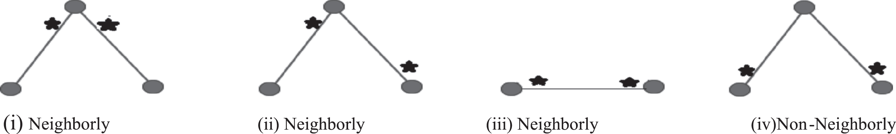
We define an incidence coloring of G to be a coloring of its incidences in which neighborly incidences are assigned different colors. The incidence coloring number of G, denoted by I (G), is the smallest number of colors in an incidence coloring.
Definition 2.2 [11]. Let (V, E) be a graph. Then G = (V, E, I) is called an incidence graph, where I ⊆ V × E. We note that if V ={ u, v } , E = { uv } and I ={ (v, uv) }, then (V, E, I) is an incidence graph even though (u, uv) ∉ I.
Definition 2.3 [11]. Let G = (V, E, I) be an incidence graph. If (u, vw) ∈ I, then (u, vw) is called an incidence pair or simply a pair. If (u, uv) , (v, uv) , (v, vw) , (w, vw) ∈ I, then uv and vw are called adjacent edges.
Definition 2.4 [5]. Let G = (V, E) be a graph and σ be a fuzzy subset of V and μ be a fuzzy subset of E (E ⊆ V × V). Let ψ be a fuzzy subset of V × E. If ψ (v, e) ⩽ σ (v) ∧ μ (e) for all v ∈ V and e ∈ E, then ψ is called a Fuzzy Incidence (FI) of G.
Definition 2.5 [6]. Let G = (V, E) be a graph and (σ, μ) be a fuzzy subgraph of G. If ψ is a Fuzzy Incidence of G, then
Definition 2.6 [27]. An incidence coloring of Fuzzy Incidence Graph
Definition 2.7 [27]. Let
i. ∨φ = ψ
ii.
iii. for each, u ∈ σ and for each pair of strongly adjacent Fuzzy Incidences ψ toward u, ψ ∈ I (G). φi [ψ (v, e)] ∧ φj [ψ (u, f)] = 0 ∀i
That C is said to be k- Fuzzy Incidence Coloring (FIC).
Definition 2.8 [27]. The minimum number of colors needed for an incidence coloring of a fuzzy graph is known as Fuzzy Incidence Chromatic Number (FICN) or Fuzzy Incidence Coloring Number of
Definition 2.9 [10]. Let G1 (σ1, μ1) and G2 (σ2, μ2) be two fuzzy graphs with underlying vertex sets V1 and V2 and edge sets E1 and E2 respectively. Then cartesian product of G1 and G2 is pair of functions (σ1 × σ2, μ1 × μ2) with underlying vertex set V = V1× V2 = { (u1, v1) ; u1∈V1 and v1∈V2 }, and underlying edge set E = E1× E2 = { (u1, v1) (u2, v2) ; u1 = u2, (v1, v2) ∈E2 or (u1, u2) ∈E1, v1 = v2 } with
3Fuzzy Incidence Coloring Number on cartesian product graphs
The FICN on the cartesian product of some FIGs such as
Definition: 3.1. Let
and whose fuzzy subsets σ1 × σ2ofV, μ1 × μ2ofE and ψ1 × ψ2ofΨ must defined as follows
• (σ1 × σ2) (v1, t1) ⩽ σ1 (v1) ∧ σ2 (t1) , where v1ɛV1 and t1ɛV2
• (μ1 × μ2) (v1, t1) (v2, t2) ⩽ σ1 (v1) ∧ μ2 (t1, t2) , where t1 = t2 and (v1, v2) ɛE2 ⩽μ1 (t1, t2) ∧ σ2 (v1) , where (t1, t2) ɛE1 and v1 = v2
•
Then the Fuzzy Incidence Graph
An example for the Definition 3.1 is illustrated below.
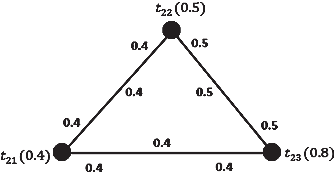
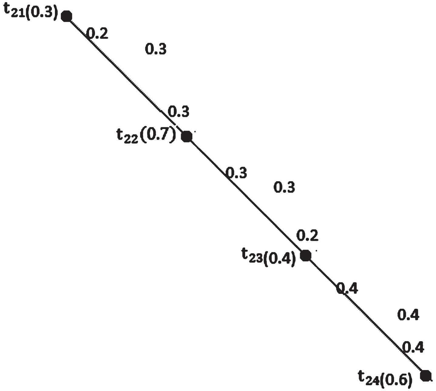
Example 3.1. Let
Fig. 3.1
FIP
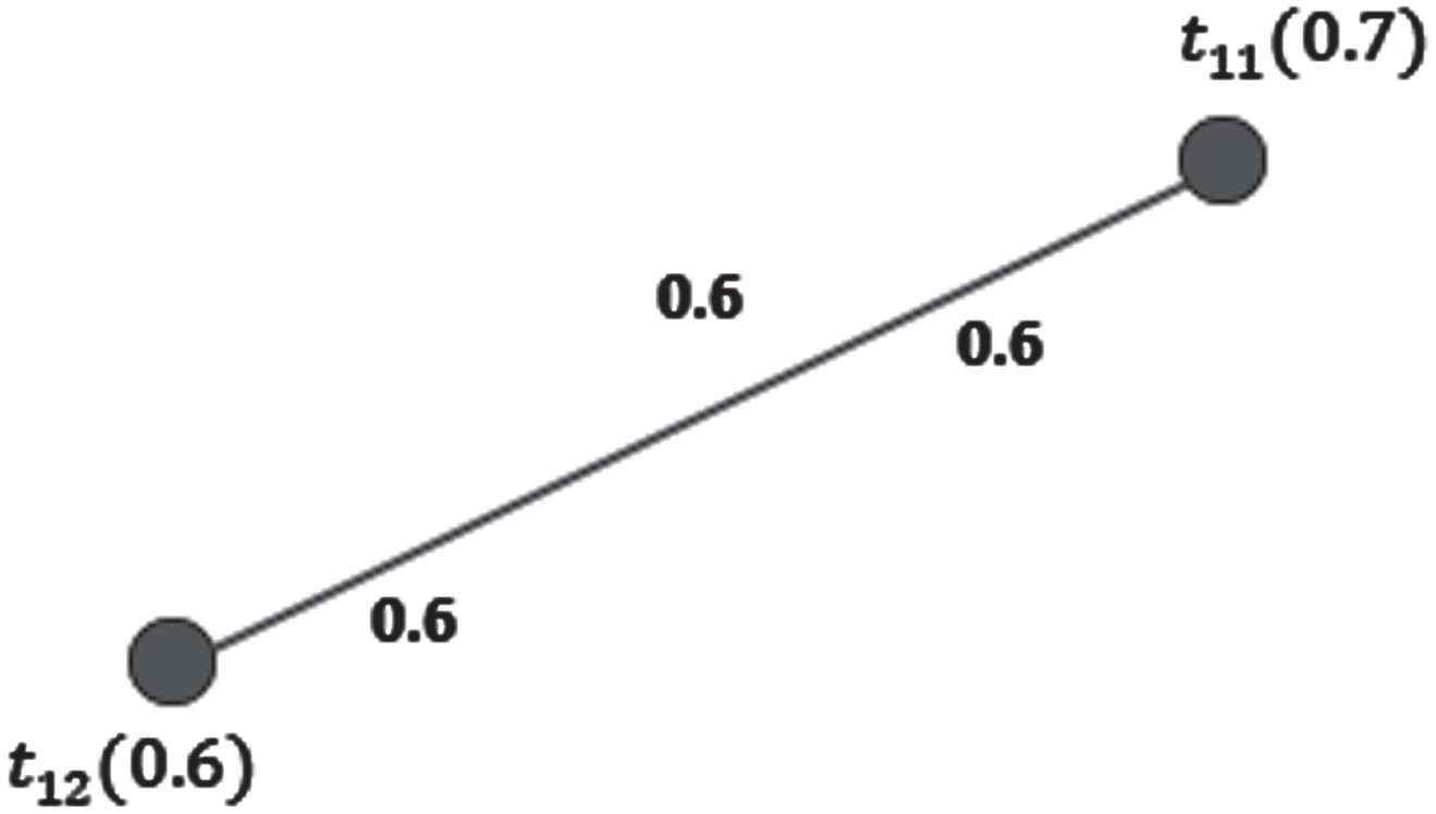
Fig. 3.2
Fuzzy Incidence cycle
Let V1, E1, FI1 are the vertex set, edge set and Fuzzy Incidence pair set of
| V1 | t11 | t12 |
| σ1 | 0.7 | 0.6 |
| E1 | t11t12 |
| μ1 | 0.6 |
| FI1 | (t11, t11t12) | (t12, t11t12) |
| ψ1 | 0.6 | 0.6 |
Let V2, E2, FI2 are the vertex set, edge set and Fuzzy Incidence pair set of
| V2 | t21 | t22 | t23 |
| σ2 | 0.4 | 0.5 | 0.8 |
| E2 | t21t22 | t22t23 | t21t23 |
| μ2 | 0.4 | 0.5 | 0.4 |
| FI2 | (t21, t21t22) | (t22, t21t22) | (t22, t22t23) |
| ψ2 | 0.4 | 0.4 | 0.5 |
| FI2 | (t23, t22t23) | (t23, t21t23) | (t21, t21t23) |
| ψ2 | 0.5 | 0.4 | 0.4 |
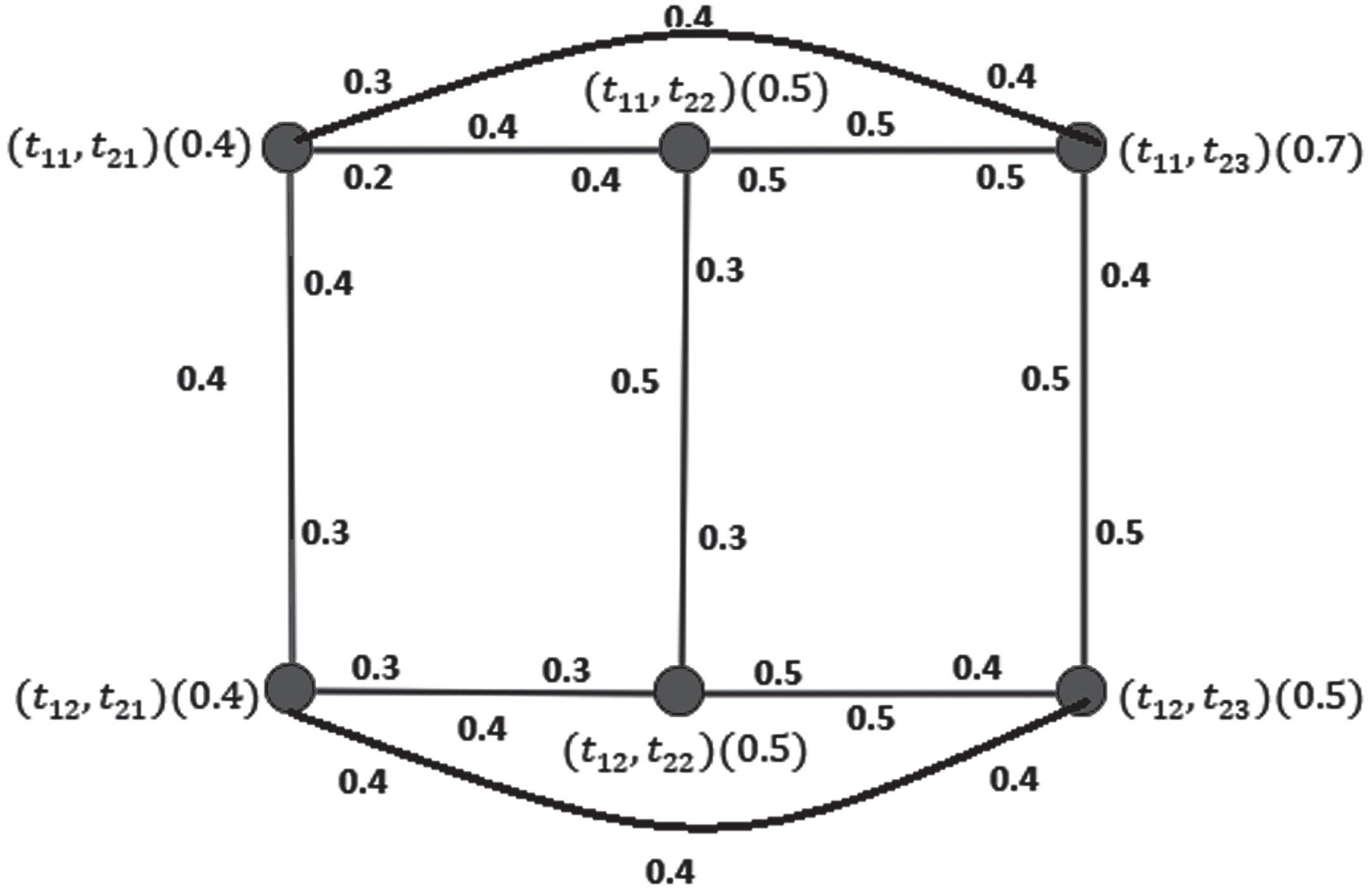
Now taking the cartesian product of FIP
i. (σ1 × σ2) (v1, t1) ⩽ σ1 (v1) ∧ σ2 (t1)
ii. (μ1 × μ2) [(v1, t1) (v2, t2)] ⩽ (σ1 × σ2) (v1, t1) ∧ (σ1 × σ2) (v2, t2)
iii. (ψ1 × ψ2) [(v1, t1) , (v1, t1) (v2, t2)] ⩽ (σ1 × σ2) (v1, t1) ∧ (μ1 × μ2) [(v1, t1) (v2, t2)]
Here, (σ1 × σ2) (t11, t21) ⩽ σ1 (t11) ∧ σ2 (t21) ⩽ 0.7 ∧ 0.4 ⩽ 0.4
Fig. 3.3
Cartesian product of
Proof. Let
Let σ1, σ2 be the Fuzzy Incidence subsets of the vertex sets V1, V2, μ1, μ2 be the Fuzzy Incidence subsets of the edge sets E1, E2, and ψ1, ψ2 be the Fuzzy Incidence subsets of the Fuzzy Incidence pair sets Ψ1, Ψ2.
By Definition 3.1, the cartesian product of FIGs,
Thus σ = σ1 × σ2 is the Fuzzy Incidence subset of the vertex set V = V1 × V2, μ = μ1 × μ2 is the Fuzzy Incidence subset of the edge set E = E1 × E2 and ψ1 × ψ2 is the Fuzzy Incidence subset of the Fuzzy Incidence pair set Ψ = Ψ1 × Ψ2. Therefore
Hence the cartesian product of any two FIGs is also a FIG.■
Theorem 3.1. The FICN for the cartesian product of FIPs
Proof. Let
By Definition 3.1 and Proposition 3.1, the cartesian product of any two FIGs must satisfies the following
i. (σ1 × σ2) (v1, t1) ⩽ σ1 (v1) ∧ σ2 (t1)
ii. (μ1 × μ2) [(v1, t1) (v2, t2)] ⩽ (σ1 × σ2) (v1, t1) ∧ (σ1 × σ2) (v2, t2)
iii. (ψ1 × ψ2) [(v1, t1) , (v1, t1) (v2, t2) ⩽ (σ1 × σ2) (v1, t1) ∧ (μ1 × μ2) [(v1, t1) (v2, t2)]
Let the adjacent FIs of ψ [(v1, t1) , (v1, t1) (v1t1, v1t2)] are ψ [(v1, t2) , (v1, t1) (v1t1, v1t2)], ψ [(v1, t2) , (v1, t2) (v1t2, v2t2)], ψ [(v1, t1) , (v1, t1) (v1t1, v2t1)], ψ [(v2, t1) , (v1, t1) (v1t1, v1t2)], . . . . By Definition 2.7, color 1 for the FI ψ [(v1, t1) , (v1, t1) (v1t1, v1t2) and distinct colors for the adjacent incidences. It is impossible to color adjacent FIs in the same color. Color all of the FIs of the cartesian product of the FIG with minimum colors in the same way. Since the two FIPs
• If m = 2orn = 2 :
• Here the products will result as a single row or single column mesh such that by coloring the adjacent FIs it is sufficient to have exactly 4 colors. Thus
• If m ⩾ 3 and n ⩾ m:
Here is the cartesian product graph with m × n rows and columns as a mesh. In this graph, the number of rows or columns is 3 and above such that exactly 6 colors are needed to color all the adjacent incidences of the mesh. Thus
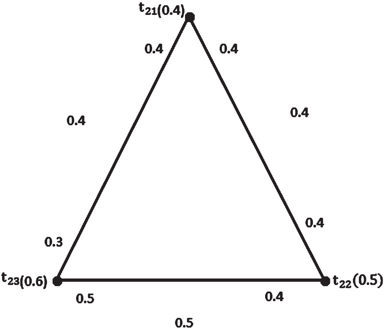
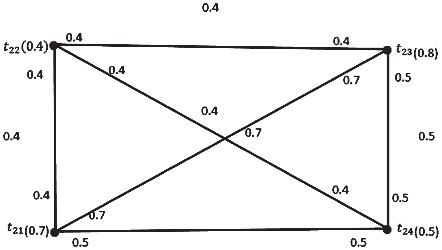
Example 3.2. Let us consider two FIPs
Fig. 3.4
FIP
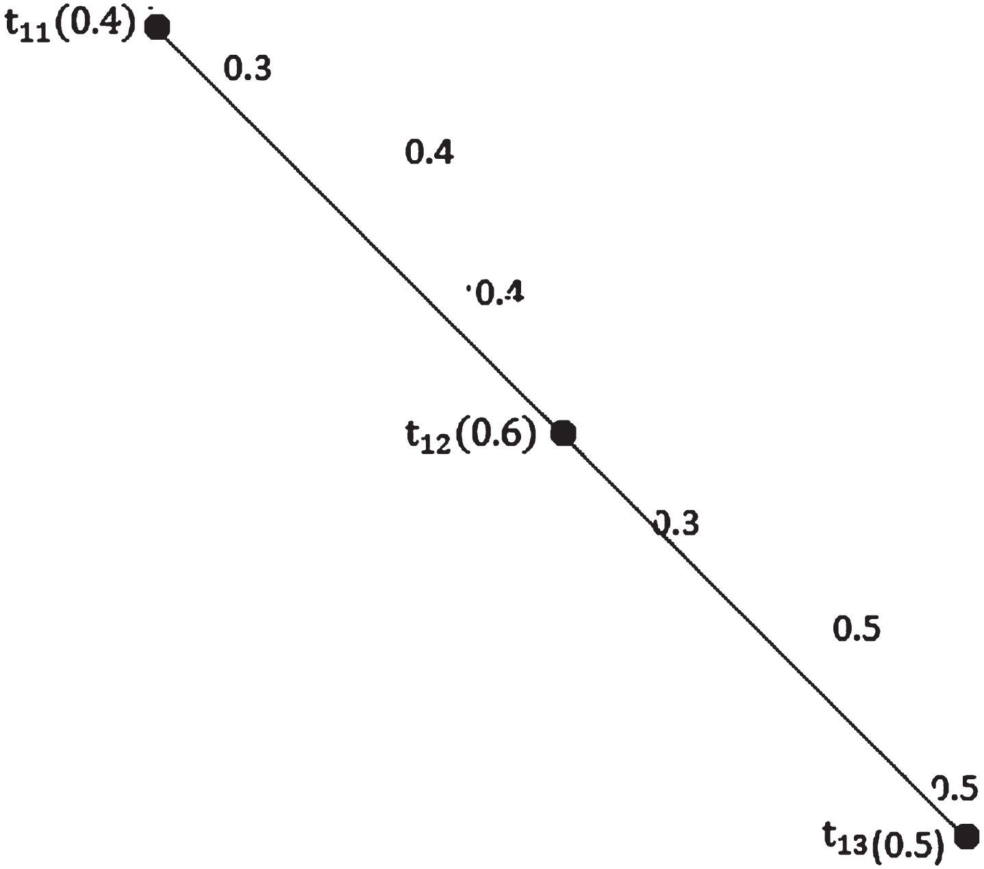
Fig. 3.5
FIP
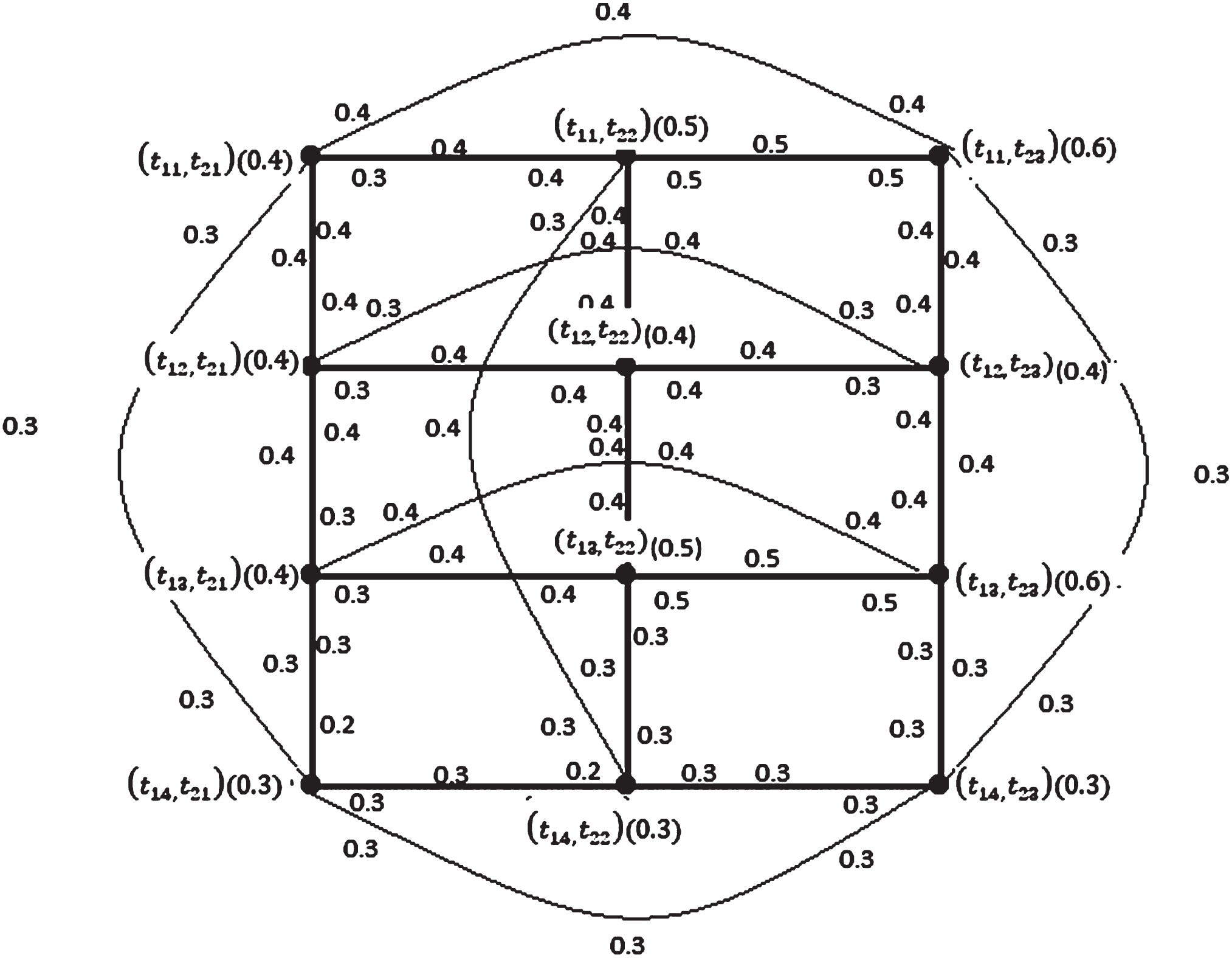
Applying cartesian product of two FIPs
i. (σ1 × σ2) (v1, t1) ⩽ σ1 (v1) ∧ σ2 (t1)
ii. (μ1 × μ2) [(v1, t1) (v2, t2)] ⩽ (σ1 × σ2) (v1, t1) ∧ (σ1 × σ2) (v2, t2)
iii. (ψ1 × ψ2) [(v1, t1) , (v1, t1) (v2, t2) ⩽ (σ1 × σ2) (v1, t1) ∧ (μ1 × μ2) [(v1, t1) (v2, t2)]
Fig. 3.6
Cartesian product of FIPs
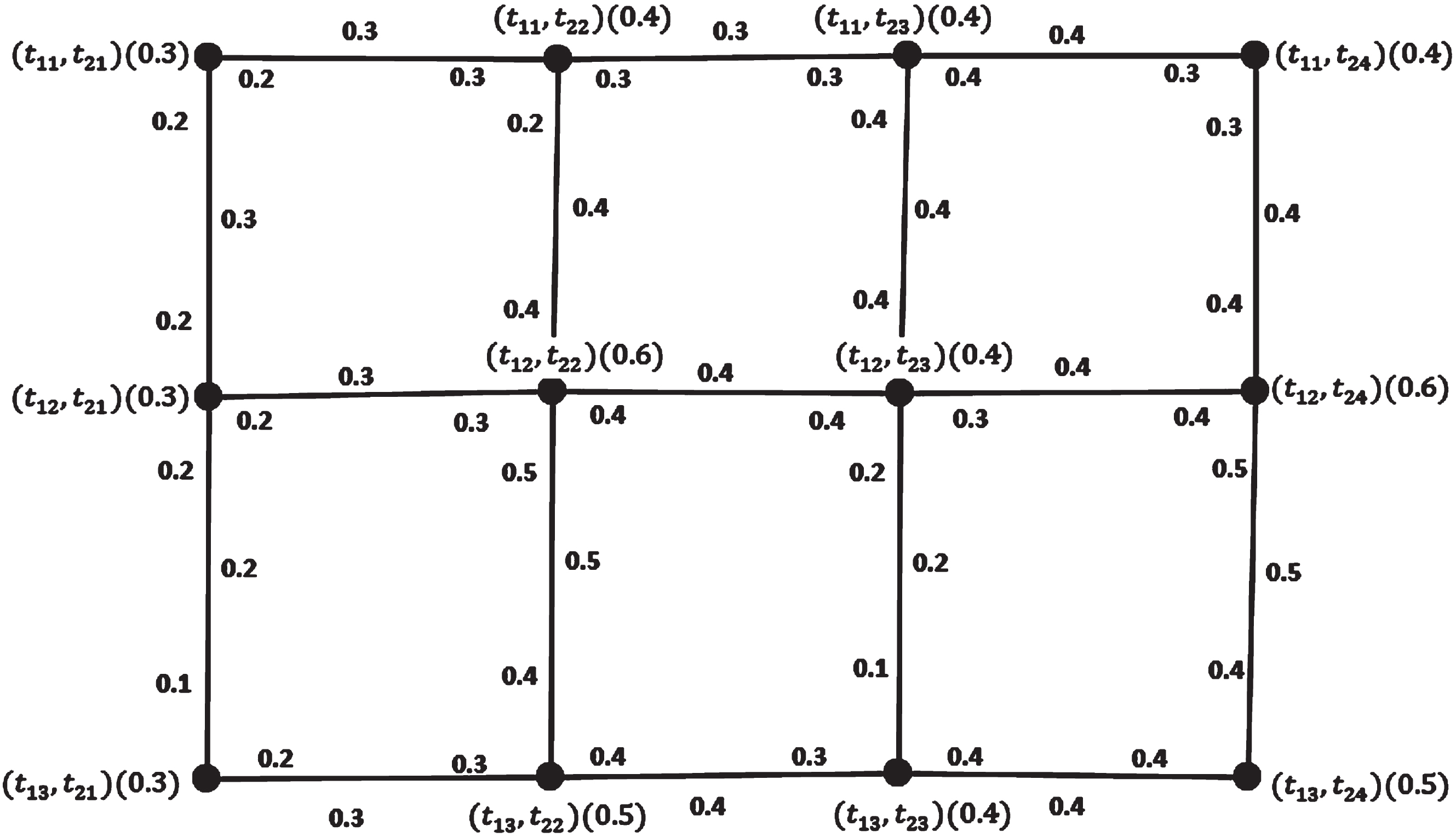
The membership values of the vertices, edges for the cartesian product of
| V | (t11, t21) | (t11, t22) | (t11, t23) | (t11, t24) | (t12, t21) | (t12, t22) |
| σ | 0.3 | 0.4 | 0.4 | 0.4 | 0.3 | 0.6 |
| V | (t12, t23) | (t12, t24) | (t13, t21) | (t13, t22) | (t13, t23) | (t13, t24) |
| σ | 0.4 | 0.6 | 0.3 | 0.5 | 0.4 | 0.5 |
| E | (t11, t21) (t11, t22) | (t11, t21) (t12, t21) | (t11, t22) (t11, t23) | (t11, t22) (t12, t22) |
| μ | 0.3 | 0.3 | 0.3 | 0.4 |
| E | (t11, t23) (t11, t24) | (t11, t23) (t12, t23) | (t11, t24) (t12, t24) | (t12, t21) (t12, t22) |
| μ | 0.4 | 0.4 | 0.4 | 0.3 |
| E | (t12, t21) (t13, t21) | (t12, t22) (t12, t23) | (t12, t22) (t13, t22) | (t12, t23) (t12, t24) |
| μ | 0.2 | 0.4 | 0.5 | 0.4 |
| E | (t12, t23) (t13, t23) | (t12, t24) (t13, t24) | (t13, t21) (t13, t22) | (t13, t22) (t13, t23) |
| μ | 0.2 | 0.5 | 0.3 | 0.4 |
| E | (t13, t23) (t13, t24) | |||
| μ | 0.4 |
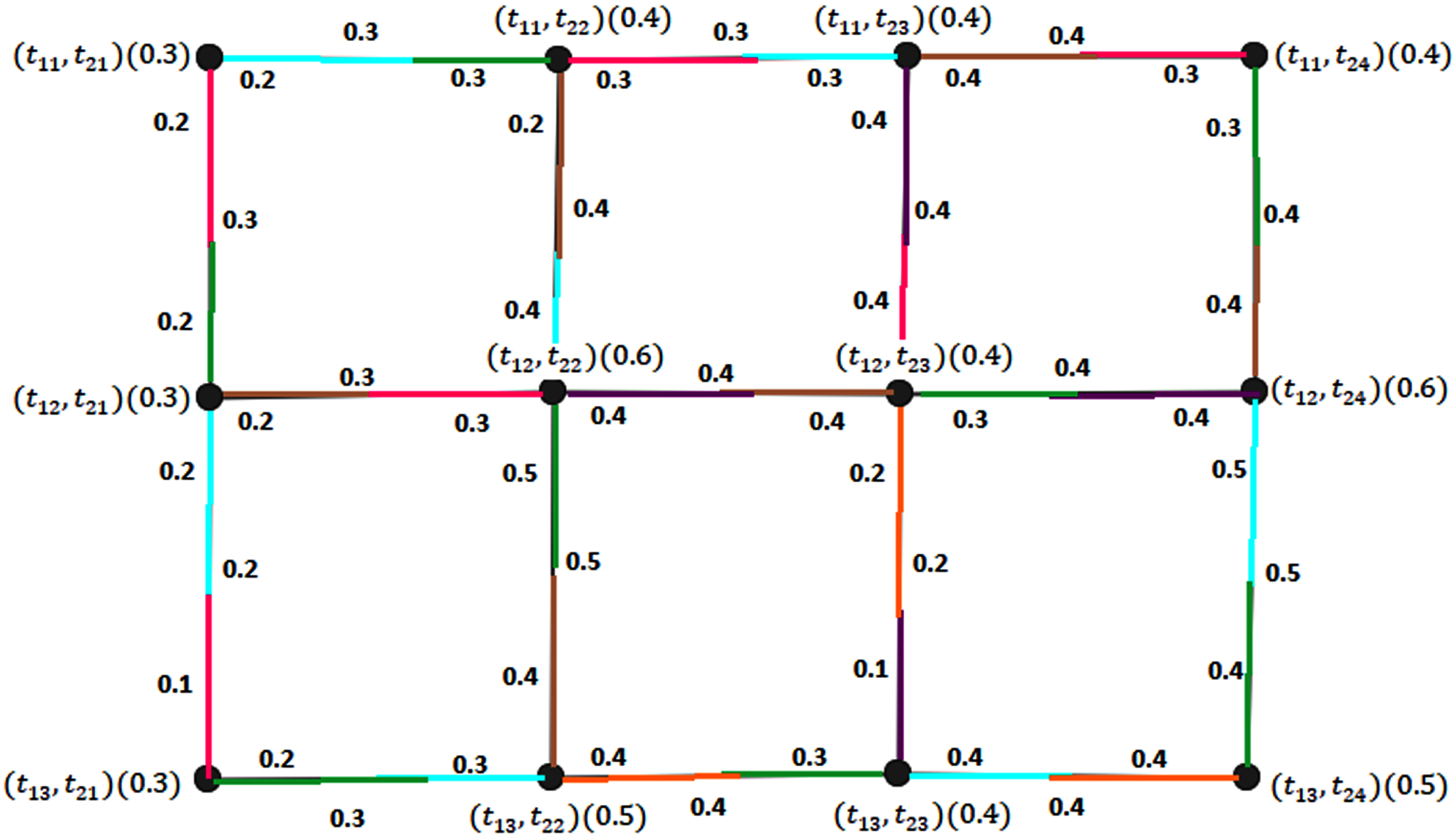
The membership functions of the FIs are represented as φ1, φ2, φ3, φ4, φ5, φ6 in Table 3.1.
Table 3.1
Membership functions of Fuzzy Incidence pairs of
| Fuzzy incidences | φ1 | φ2 | φ3 | φ4 | φ5 | φ6 | Max |
| ψ [(t11, t21) , (t11, t21) (t11, t22)] | 0.2 | 0 | 0 | 0 | 0 | 0 | 0.2 |
| ψ [(t11, t21) , (t11, t21) (t12, t21)] | 0 | 0.2 | 0 | 0 | 0 | 0 | 0.2 |
| ψ [(t12, t21) , (t11, t21) (t12, t21)] | 0 | 0 | 0.2 | 0 | 0 | 0 | 0.2 |
| ψ [(t12, t21) , (t12, t21) (t12, t22)] | 0 | 0 | 0 | 0.2 | 0 | 0 | 0.2 |
| ψ [(t12, t21) , (t12, t21) (t13, t21)] | 0.2 | 0 | 0 | 0 | 0 | 0 | 0.2 |
| ψ [(t13, t21) , (t12, t21) (t13, t21)] | 0 | 0.1 | 0 | 0 | 0 | 0 | 0.1 |
| ψ [(t13, t21) , (t13, t21) (t13, t22)] | 0 | 0 | 0.2 | 0 | 0 | 0 | 0.2 |
| ψ [(t11, t22) , (t11, t21) (t11, t22)] | 0 | 0 | 0.3 | 0 | 0 | 0 | 0.3 |
| ψ [(t11, t22) , (t11, t21) (t12, t22)] | 0 | 0 | 0 | 0.2 | 0 | 0 | 0.2 |
| ψ [(t11, t22) , (t11, t21) (t11, t23)] | 0 | 0.3 | 0 | 0 | 0 | 0 | 0.3 |
| ψ [(t12, t22) , (t11, t22) (t12, t22)] | 0.4 | 0 | 0 | 0 | 0 | 0 | 0.4 |
| ψ [(t12, t22) , (t12, t21) (t12, t22)] | 0 | 0.3 | 0 | 0 | 0 | 0 | 0.3 |
| ψ [(t12, t22) , (t12, t22) (t12, t23)] | 0 | 0 | 0 | 0 | 0.4 | 0 | 0.4 |
| ψ [(t12, t22) , (t12, t22) (t13, t22)] | 0 | 0 | 0.5 | 0 | 0 | 0 | 0.5 |
| ψ [(t13, t22) , (t12, t22) (t13, t22)] | 0 | 0 | 0 | 0.4 | 0 | 0 | 0.4 |
| ψ [(t13, t22) , (t13, t21) (t13, t22)] | 0.3 | 0 | 0 | 0 | 0 | 0 | 0.3 |
| ψ [(t13, t22) , (t13, t22) (t13, t23)] | 0 | 0 | 0 | 0 | 0 | 0.4 | 0.4 |
| ψ [(t11, t23) , (t11, t22) (t11, t23)] | 0.3 | 0 | 0 | 0 | 0 | 0 | 0.3 |
| ψ [(t11, t23) , (t11, t23) (t11, t24)] | 0 | 0 | 0 | 0.4 | 0 | 0 | 0.4 |
| ψ [(t11, t23) , (t11, t23) (t12, t23)] | 0 | 0 | 0 | 0 | 0.4 | 0 | 0.4 |
| ψ [(t12, t23) , (t11, t23) (t12, t23)] | 0 | 0.4 | 0 | 0 | 0 | 0 | 0.4 |
| ψ [(t12, t23) , (t12, t22) (t12, t23)] | 0 | 0 | 0 | 0.4 | 0 | 0 | 0.4 |
| ψ [(t12, t23) , (t12, t22) (t12, t24)] | 0 | 0 | 0.4 | 0 | 0 | 0 | 0.4 |
| ψ [(t12, t23) , (t12, t23) (t13, t23)] | 0 | 0 | 0 | 0 | 0 | 0.2 | 0.2 |
| ψ [(t13, t23) , (t12, t23) (t13, t23)] | 0 | 0 | 0 | 0 | 0.1 | 0 | 0.1 |
| ψ [(t13, t23) , (t13, t22) (t13, t23)] | 0 | 0 | 0.3 | 0 | 0 | 0 | 0.3 |
| ψ [(t13, t23) , (t13, t23) (t13, t24)] | 0.4 | 0 | 0 | 0 | 0 | 0 | 0.4 |
| ψ [(t11, t24) , (t11, t23) (t11, t24)] | 0 | 0.3 | 0 | 0 | 0 | 0 | 0.3 |
| ψ [(t11, t24) , (t11, t24) (t12, t24)] | 0 | 0 | 0.3 | 0 | 0 | 0 | 0.3 |
| ψ [(t12, t24) , (t11, t24) (t12, t24)] | 0 | 0 | 0 | 0.4 | 0 | 0 | 0.4 |
| ψ [(t12, t24) , (t12, t23) (t12, t24)] | 0 | 0 | 0 | 0 | 0.4 | 0 | 0.4 |
| ψ [(t12, t24) , (t12, t24) (t13, t24)] | 0.5 | 0 | 0 | 0 | 0 | 0 | 0.5 |
| ψ [(t13, t24) , (t12, t24) (t13, t24)] | 0 | 0 | 0.4 | 0 | 0 | 0 | 0.4 |
| ψ [(t13, t24) , (t13, t23) (t13, t24)] | 0 | 0 | 0 | 0 | 0 | 0.4 | 0.4 |
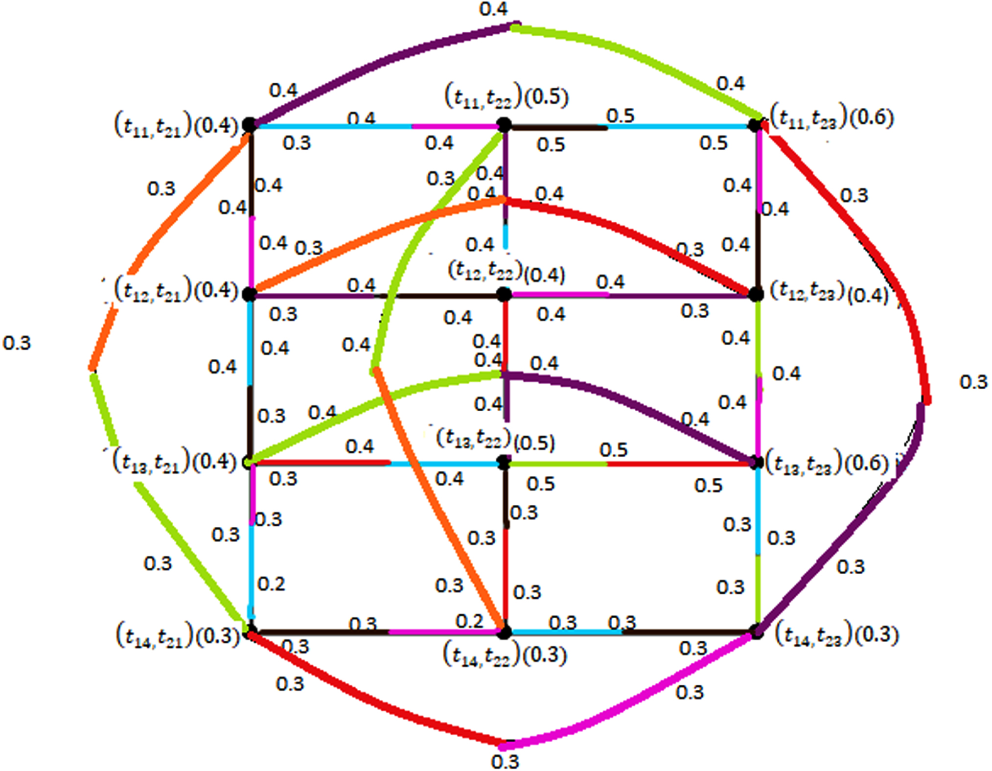
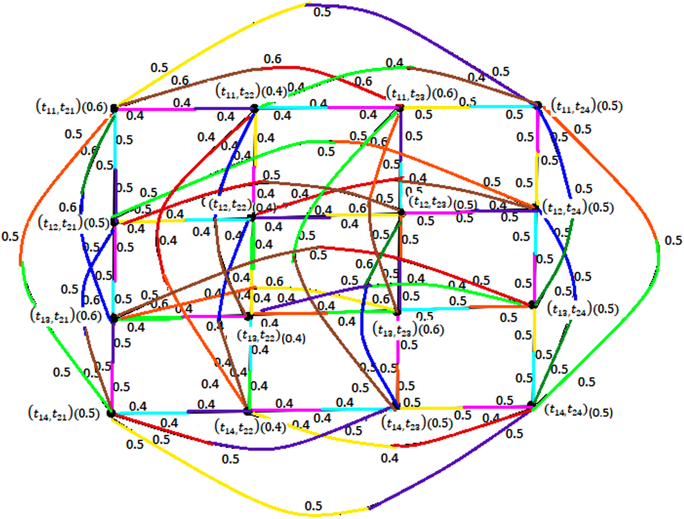
Thus
As a result, the partitions satisfy the FIC definition’s criteria by [27]. In Fig. 3.7, the FIs in φ1 are colored blue, φ2 are colored pink, φ3 are colored green, φ4 are colored brown, φ5 are colored violet, and φ6 are colored orange.
There fore
Fig. 3.7
FIC on the cartesian product of FIPs
Theorem 3.2. The FICN for the cartesian product of the FIP
Proof. Let
Assume that σ1 ={ v1, v2, v3, …, vm } be the vertex set of degree
By Proposition 3.1, the cartesian product of any two FIGs must satisfy the following conditions
i. (σ1 × σ2) (v1, t1) ⩽ σ1 (v1) ∧ σ2 (t1)
ii. (μ1 × μ2) [(v1, t1) (v2, t2)] ⩽ (σ1 × σ2) (v1, t1) ∧ (σ1 × σ2) (v2, t2)
iii. (ψ1 × ψ2) [(v1, t1) , (v1, t1) (v2, t2) ⩽ (σ1 × σ2) (v1, t1) ∧ (μ1 × μ2) [(v1, t1) (v2, t2)]
Thus σ = σ1 × σ2 is the vertex set of the cartesian product of FIP and Fuzzy Incidence cycle with mn vertices and maximum degree Δ′ = 4 . μ = μ1 × μ2 be the edge set incident with σ and ψ = ψ1 × ψ2 be the FI set of σ and μ.
Color all of the adjacent FIs of the cartesian product of the FIG with minimum colors by Definition 2.7.
By Theorem 3.1, the cartesian product for any two FIPs with Δ′ = 4 needs exactly 6 colors. Since the cartesian product between any two FIGs will be constructed as a mesh initially then the edges may be incident with vertices if the graph is a Fuzzy Incidence cycle.
Thus the FICN of the cartesian product between FIP and Fuzzy Incidence cycle has its upper bound 8, i.e.
For every
Theorem 3.3. If
Proof: Let
Applying the cartesian product on
Suppose in
The FICN required to color the cartesian product of
Hence
Example 3.3. Let us consider two Fuzzy Incidence cycles
Fig. 3.8
Fuzzy incidence cycle
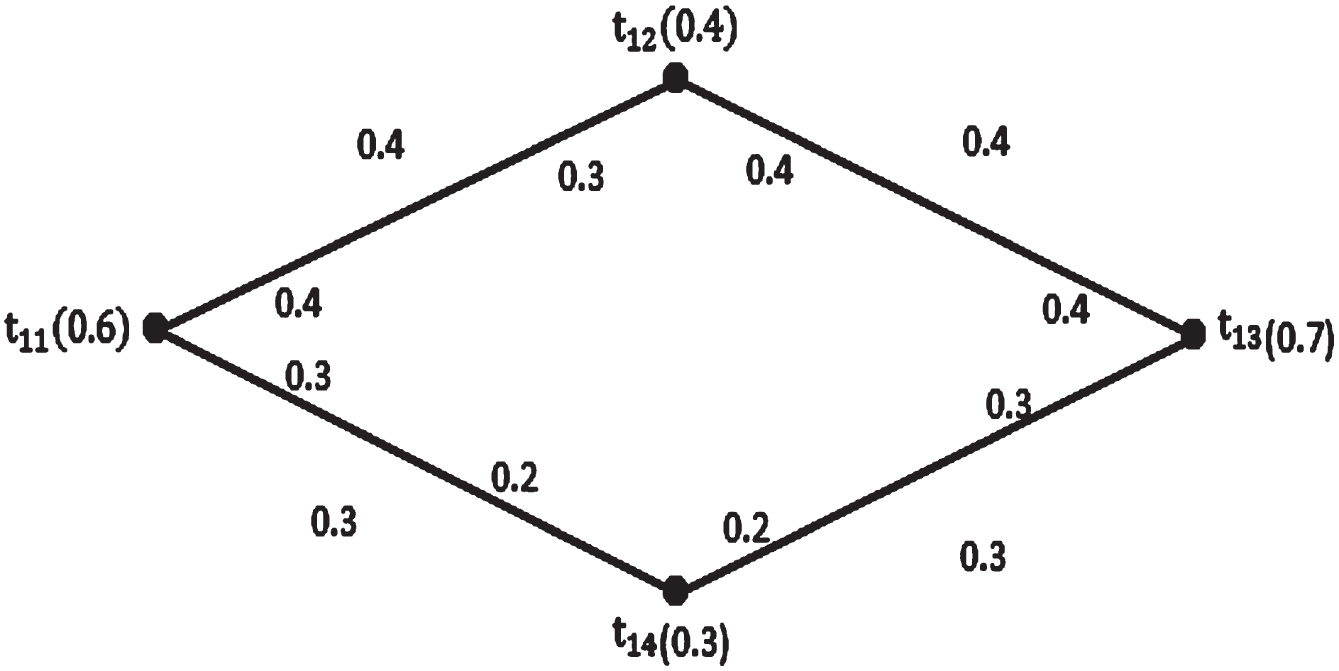
Fig. 3.9
Fuzzy incidence cycle
Applying the cartesian product of Fuzzy Incidence cycles
i. (σ1 × σ2) (v1, t1) ⩽ σ1 (v1) ∧ σ2 (t1)
ii. (μ1 × μ2) [(v1, t1) (v2, t2)] ⩽ (σ1 × σ2) (v1, t1) ∧ (σ1 × σ2) (v2, t2)
iii. (ψ1 × ψ2) [(v1, t1) , (v1, t1) (v2, t2) ⩽ (σ1 × σ2) (v1, t1) ∧ (μ1 × μ2) [(v1, t1) (v2, t2)]
Fig. 3.10
Cartesian product of
The membership values of the vertex set, edge set for the cartesian product of
Table 3.2 represents the membership functions of the Fuzzy Incidences as φ1, φ2, φ3, φ4, φ5, φ6 and φ7.
Table 3.2
Membership functions of the Fuzzy Incidences pairs of
| Fuzzy incidences | φ1 | φ2 | φ3 | φ4 | φ5 | φ6 | φ7 | Max |
| ψ [(t11, t21) , (t11, t21) (t11, t22)] | 0.3 | 0 | 0 | 0 | 0 | 0 | 0 | 0.3 |
| ψ [(t11, t21) , (t11, t21) (t11, t23)] | 0 | 0 | 0.4 | 0 | 0 | 0 | 0 | 0.4 |
| ψ [(t11, t21) , (t11, t21) (t12, t21)] | 0 | 0 | 0 | 0 | 0 | 0.4 | 0 | 0.4 |
| ψ [(t11, t21) , (t11, t21) (t14, t21)] | 0 | 0 | 0 | 0 | 0 | 0 | 0.3 | 0.3 |
| ψ [(t11, t22) , (t11, t21) (t11, t22)] | 0 | 0.4 | 0 | 0 | 0 | 0 | 0 | 0.4 |
| ψ [(t11, t22) , (t11, t22) (t11, t23)] | 0 | 0 | 0 | 0 | 0 | 0.5 | 0 | 0.5 |
| ψ [(t11, t22) , (t11, t22) (t12, t22)] | 0 | 0 | 0.4 | 0 | 0 | 0 | 0 | 0.4 |
| ψ [(t11, t22) , (t11, t22) (t14, t22)] | 0 | 0 | 0 | 0.3 | 0 | 0 | 0 | 0.3 |
| ψ [(t11, t23) , (t11, t22) (t11, t23)] | 0.5 | 0 | 0 | 0 | 0 | 0 | 0 | 0.5 |
| ψ [(t11, t23) , (t11, t23) (t12, t23)] | 0 | 0.4 | 0 | 0 | 0 | 0 | 0 | 0.4 |
| ψ [(t11, t23) , (t11, t21) (t11, t23)] | 0 | 0 | 0 | 0.4 | 0 | 0 | 0 | 0.4 |
| ψ [(t11, t23) , (t11, t23) (t14, t23)] | 0 | 0 | 0 | 0 | 0.3 | 0 | 0 | 0.3 |
| ψ [(t12, t21) , (t11, t21) (t12, t21)] | 0 | 0.4 | 0 | 0 | 0 | 0 | 0 | 0.4 |
| ψ [(t12, t21) , (t12, t21) (t12, t22)] | 0 | 0 | 0.3 | 0 | 0 | 0 | 0 | 0.3 |
| ψ [(t12, t21) , (t12, t21) (t12, t23)] | 0 | 0 | 0 | 0 | 0 | 0 | 0.3 | 0.3 |
| ψ [(t12, t21) , (t12, t21) (t13, t21)] | 0.4 | 0 | 0 | 0 | 0 | 0 | 0 | 0.4 |
| ψ [(t12, t22) , (t12, t21) (t12, t22)] | 0 | 0 | 0 | 0 | 0 | 0.4 | 0 | 0.4 |
| ψ [(t12, t22) , (t11, t22) (t12, t22)] | 0.4 | 0 | 0 | 0 | 0 | 0 | 0 | 0.4 |
| ψ [(t12, t22) , (t12, t22) (t12, t23)] | 0 | 0.4 | 0 | 0 | 0 | 0 | 0 | 0.4 |
| ψ [(t12, t22) , (t12, t22) (t13, t22)] | 0 | 0 | 0 | 0 | 0.4 | 0 | 0 | 0.4 |
| ψ [(t12, t23) , (t12, t22) (t12, t23)] | 0 | 0 | 0.3 | 0 | 0 | 0 | 0 | 0.3 |
| ψ [(t12, t23) , (t11, t23) (t12, t23)] | 0 | 0 | 0 | 0 | 0 | 0.4 | 0 | 0.4 |
| ψ [(t12, t23) , (t12, t21) (t12, t23)] | 0 | 0 | 0 | 0 | 0.3 | 0 | 0 | 0.3 |
| ψ [(t12, t23) , (t12, t23) (t13, t23)] | 0 | 0 | 0 | 0.4 | 0 | 0 | 0 | 0.4 |
| ψ [(t13, t21) , (t12, t21) (t13, t21)] | 0 | 0 | 0 | 0 | 0 | 0.3 | 0 | 0.3 |
| ψ [(t13, t21) , (t13, t21) (t13, t22)] | 0 | 0 | 0 | 0 | 0.3 | 0 | 0 | 0.3 |
| ψ [(t13, t21) , (t13, t21) (t13, t23)] | 0 | 0 | 0 | 0.4 | 0 | 0 | 0 | 0.4 |
| ψ [(t13, t21) , (t13, t21) (t14, t21)] | 0 | 0.3 | 0 | 0 | 0 | 0 | 0 | 0.3 |
| ψ [(t13, t22) , (t13, t21) (t13, t22)] | 0.4 | 0 | 0 | 0 | 0 | 0 | 0 | 0.4 |
| ψ [(t13, t22) , (t13, t22) (t13, t23)] | 0 | 0 | 0 | 0.5 | 0 | 0 | 0 | 0.5 |
| ψ [(t13, t22) , (t12, t22) (t13, t22)] | 0 | 0 | 0.4 | 0 | 0 | 0 | 0 | 0.4 |
| ψ [(t13, t22) , (t13, t22) (t14, t22)] | 0 | 0 | 0 | 0 | 0 | 0.3 | 0 | 0.3 |
| ψ [(t13, t23) , (t13, t22) (t13, t23)] | 0 | 0 | 0 | 0 | 0.5 | 0 | 0 | 0.5 |
| ψ [(t13, t23) , (t13, t21) (t13, t23)] | 0 | 0 | 0.4 | 0 | 0 | 0 | 0 | 0.4 |
| ψ [(t13, t23) , (t12, t23) (t13, t23)] | 0 | 0.4 | 0 | 0 | 0 | 0 | 0 | 0.4 |
| ψ [(t13, t23) , (t13, t23) (t14, t23)] | 0.3 | 0 | 0 | 0 | 0 | 0 | 0 | 0.3 |
| ψ [(t14, t21) , (t13, t21) (t14, t21)] | 0.2 | 0 | 0 | 0 | 0 | 0 | 0 | 0.2 |
| ψ [(t14, t21) , (t11, t21) (t14, t21)] | 0 | 0 | 0 | 0.3 | 0 | 0 | 0 | 0.3 |
| ψ [(t14, t21) , (t14, t21) (t14, t22)] | 0 | 0 | 0 | 0 | 0 | 0.3 | 0 | 0.3 |
| ψ [(t14, t21) , (t14, t21) (t14, t23)] | 0 | 0 | 0 | 0 | 0.3 | 0 | 0 | 0.3 |
| ψ [(t14, t22) , (t14, t21) (t14, t22)] | 0 | 0.2 | 0 | 0 | 0 | 0 | 0 | 0.2 |
| ψ [(t14, t22) , (t13, t22) (t14, t22)] | 0 | 0 | 0 | 0 | 0.3 | 0 | 0 | 0.3 |
| ψ [(t14, t22) , (t11, t22) (t14, t22)] | 0 | 0 | 0 | 0 | 0 | 0 | 0.3 | 0.3 |
| ψ [(t14, t22) , (t14, t22) (t14, t23)] | 0.3 | 0 | 0 | 0 | 0 | 0 | 0 | 0.3 |
| ψ [(t14, t23) , (t14, t22) (t14, t23)] | 0 | 0 | 0 | 0 | 0 | 0.3 | 0 | 0.3 |
| ψ [(t14, t23) , (t14, t21) (t14, t23)] | 0 | 0.3 | 0 | 0 | 0 | 0 | 0 | 0.3 |
| ψ [(t14, t23) , (t13, t23) (t14, t23)] | 0 | 0 | 0 | 0.3 | 0 | 0 | 0 | 0.3 |
| ψ [(t14, t23) , (t11, t23) (t14, t23)] | 0 | 0 | 0.3 | 0 | 0 | 0 | 0 | 0.3 |
| V | (t11, t21) | (t11, t22) | (t11, t23) | (t12, t21) | (t12, t22) | (t12, t23) |
| σ | 0.4 | 0.5 | 0.6 | 0.4 | 0.4 | 0.4 |
| V | (t13, t21) | (t13, t22) | (t13, t23) | (t14, t21) | (t14, t22) | (t14, t23) |
| σ | 0.4 | 0.5 | 0.6 | 0.3 | 0.3 | 0.3 |
| E | (t11, t21) (t11, t22) | (t11, t21) (t12, t21) | (t11, t21) (t11, t23) | (t11, t21) (t14, t21) |
| μ | 0.4 | 0.4 | 0.4 | 0.3 |
| E | (t11, t22) (t11, t23) | (t11, t22) (t12, t22) | (t11, t22) (t14, t22) | (t11, t23) (t12, t23) |
| μ | 0.5 | 0.4 | 0.3 | 0.4 |
| E | (t11, t23) (t14, t23) | (t12, t21) (t12, t22) | (t12, t21) (t13, t21) | (t12, t21) (t12, t23) |
| μ | 0.3 | 0.4 | 0.4 | 0.4 |
| E | (t12, t22) (t12, t23) | (t12, t22) (t13, t22) | (t12, t23) (t13, t23) | (t13, t21) (t14, t21) |
| μ | 0.4 | 0.4 | 0.4 | 0.3 |
| E | (t13, t21) (t13, t22) | (t13, t21) (t13, t23) | (t13, t22) (t13, t23) | (t13, t22) (t14, t22) |
| μ | 0.4 | 0.4 | 0.5 | 0.3 |
| E | (t13, t23) (t14, t23) | (t14, t21) (t14, t22) | (t14, t21) (t14, t23) | (t14, t22) (t14, t23) |
| μ | 0.3 | 0.3 | 0.3 | 0.3 |
Thus,
According to the definition of FIC by Yamuna et al. [27], the partitions set of cartesian product
Fig. 3.11
FIC on cartesian product of
By Theorem 3.3,
Hence
Theorem 3.4. If
Proof. Let
Now by the Definition 3.1 and Proposition 3.1, the cartesian product on FIP
By Yamuna et al. [27], w.k.t the FICN for a Fuzzy Incidence complete graph is Δ′ + 1. In the cartesian product
By Definition 2.7, color the first FI of ψ by color 1. No two FIs can be colored with the same color. Using distinct colors color all the remaining adjacent FIs of
3pt
We conclude that the FICN of a cartesian product of a FIP with m ⩾ 2 vertices and a Fuzzy Incidence complete graph with n ⩾ 3 vertices ranges between
Theorem 3.5. The FICN for the cartesian product of Fuzzy Incidence cycle and Fuzzy Incidence complete graph is
Proof. Let
Let
Now by Definition 3.1, the cartesian product of
Apply the coloring for the set of each Fuzzy Incidence pair of
By Definition 2.7, color the first Fuzzy Incidence of ψ in
Hence, we conclude that the FICN for the cartesian product of
Theorem 3.6. The FICN for a cartesian product of two Fuzzy Incidence complete graphs is
Proof. As every Fuzzy Incidence pair of the cartesian product of two Fuzzy Incidence complete graphs
By Yamuna et al. [27], the FICN of a Fuzzy Incidence complete graph with n vertices and maximum degree Δ′ = n - 1 is Δ′ + 1.
Here are the two Fuzzy Incidence complete graphs with m and n vertices having maximum degree
Now coloring all the adjacent FIs of the cartesian product graph
Example 3.4. Let us consider two Fuzzy Incidence complete graphs with 4 vertices whose degree is 4 - 1 namely
Fig. 3.12
Fuzzy Incidence complete graph
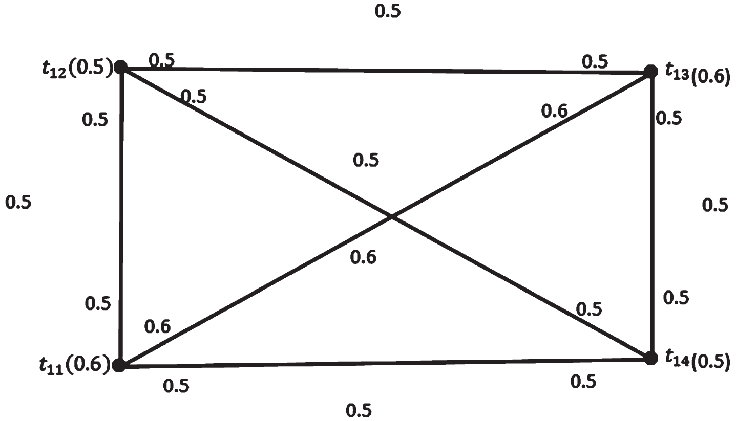
Fig. 3.13
Fuzzy Incidence complete graph
Now taking the cartesian product of
(i) (σ1 × σ2) (v1, t1) ⩽ σ1 (v1) ∧ σ2 (t1)
(ii) (μ1 × μ2) [(v1, t1) (v2, t2)] ⩽ (σ1 × σ2) (v1, t1) ∧ (σ1 × σ2) (v2, t2)
(iii) (ψ1 × ψ2) [(v1, t1) , (v1, t1) (v2, t2) ⩽ (σ1 × σ2) (v1, t1) ∧ (μ1 × μ2) [(v1, t1) (v2, t2)]
| V | (t11, t21) | (t11, t22) | (t11, t23) | (t11, t24) |
| σ | 0.6 | 0.4 | 0.6 | 0.5 |
| V | (t12, t21) | (t12, t22) | (t12, t23) | (t12, t24) |
| σ | 0.5 | 0.4 | 0.5 | 0.5 |
| V | (t13, t21) | (t13, t22) | (t13, t23) | (t13, t24) |
| σ | 0.6 | 0.4 | 0.6 | 0.5 |
| V | (t14, t21) | (t14, t22) | (t14, t23) | (t14, t24) |
| σ | 0.5 | 0.4 | 0.5 | 0.5 |
| E | (t11, t21) (t11, t22) | (t11, t21) (t11, t23) | (t11, t21) (t11, t24) | (t11, t21) (t12, t21) |
| μ | 0.4 | 0.6 | 0.5 | 0.5 |
| E | (t11, t21) (t13, t21) | (t11, t21) (t14, t21) | (t11, t22) (t11, t23) | (t11, t22) (t11, t24) |
| μ | 0.6 | 0.5 | 0.4 | 0.4 |
| E | (t11, t22) (t12, t22) | (t11, t22) (t13, t22) | (t11, t22) (t14, t22) | (t11, t23) (t11, t24) |
| μ | 0.4 | 0.4 | 0.4 | 0.5 |
| E | (t11, t23) (t12, t23) | (t11, t23) (t13, t23) | (t11, t23) (t14, t23) | (t11, t24) (t12, t24) |
| μ | 0.5 | 0.6 | 0.5 | 0.5 |
| E | (t11, t24) (t13, t24) | (t11, t24) (t14, t24) | (t12, t21) (t12, t22) | (t12, t21) (t12, t23) |
| μ | 0.5 | 0.5 | 0.4 | 0.5 |
| E | (t12, t21) (t12, t23) | (t12, t21) (t13, t21) | (t12, t21) (t14, t21) | (t12, t22) (t12, t23) |
| μ | 0.5 | 0.5 | 0.5 | 0.4 |
| E | (t12, t22) (t12, t24) | (t12, t22) (t13, t22) | (t12, t22) (t14, t22) | (t12, t23) (t12, t24) |
| μ | 0.4 | 0.4 | 0.4 | 0.5 |
| E | (t12, t23) (t13, t23) | (t12, t23) (t14, t23) | (t12, t24) (t13, t24) | (t12, t24) (t14, t24) |
| μ | 0.5 | 0.5 | 0.5 | 0.5 |
| E | (t13, t21) (t13, t22) | (t13, t21) (t14, t21) | (t13, t21) (t13, t23) | (t13, t21) (t13, t24) |
| μ | 0.4 | 0.5 | 0.6 | 0.5 |
| E | (t13, t22) (t13, t23) | (t13, t22) (t13, t24) | (t13, t22) (t14, t22) | (t13, t23) (t13, t24) |
| μ | 0.4 | 0.4s | 0.4 | 0.5 |
| E | (t13, t23) (t14, t23) | (t13, t24) (t14, t24) | (t14, t21) (t14, t22) | (t14, t21) (t14, t23) |
| μ | 0.5 | 0.5 | 0.4 | 0.5 |
| E | (t14, t21) (t14, t24) | (t14, t22) (t14, t23) | (t14, t22) (t14, t24) | (t14, t23) (t14, t24) |
| μ | 0.5 | 0.4 | 0.4 | 0.5 |
The cartesian product graph
Fig. 3.14
Cartesian product of
Table 3.3 represents the membership functions of the FIs as φ1, φ2, φ3, φ4, φ5, φ6, φ7, φ8, φ9 and φ10.
Table 3.3
Membership functions of FIs on
| Fuzzy Incidences | φ1 | φ2 | φ3 | φ4 | φ5 | φ6 | φ7 | φ8 | φ9 | φ10 | Max |
| ψ [(t11, t21) , (t11, t21) (t11, t22)] | 0.4 | 0 | 0 | 0 | 0 | 0 | 0 | 0 | 0 | 0 | 0.4 |
| ψ [(t11, t21) , (t11, t21) (t11, t23)] | 0 | 0.6 | 0 | 0 | 0 | 0 | 0 | 0 | 0 | 0 | 0.6 |
| ψ [(t11, t21) , (t11, t21) (t11, t24)] | 0 | 0 | 0.5 | 0 | 0 | 0 | 0 | 0 | 0 | 0 | 0.5 |
| ψ [(t11, t21) , (t11, t21) (t12, t21)] | 0 | 0 | 0 | 0.5 | 0 | 0 | 0 | 0 | 0 | 0 | 0.5 |
| ψ [(t11, t21) , (t11, t21) (t13, t21)] | 0 | 0 | 0 | 0 | 0.6 | 0 | 0 | 0 | 0 | 0 | 0.6 |
| ψ [(t11, t21) , (t11, t21) (t14, t21)] | 0 | 0 | 0 | 0 | 0 | 0.5 | 0 | 0 | 0 | 0 | 0.5 |
| ψ [(t11, t22) , (t11, t21) (t11, t22)] | 0 | 0 | 0 | 0 | 0 | 0 | 0.4 | 0 | 0 | 0 | 0.4 |
| ψ [(t11, t22) , (t11, t22) (t11, t23)] | 0 | 0 | 0 | 0.4 | 0 | 0 | 0 | 0 | 0 | 0 | 0.4 |
| ψ [(t11, t22) , (t11, t22) (t11, t24)] | 0 | 0 | 0 | 0 | 0 | 0 | 0 | 0.4 | 0 | 0 | 0.4 |
| ψ [(t11, t22) , (t11, t22) (t12, t22)] | 0 | 0 | 0.4 | 0 | 0 | 0 | 0 | 0 | 0 | 0 | 0.4 |
| ψ [(t11, t22) , (t11, t22) (t13, t22)] | 0 | 0 | 0 | 0 | 0 | 0 | 0 | 0.4 | 0 | 0 | 0.4 |
| ψ [(t11, t22) , (t11, t22) (t14, t22)] | 0 | 0 | 0 | 0 | 0 | 0 | 0 | 0 | 0 | 0.4 | 0.4 |
| ψ [(t11, t23) , (t11, t21) (t11, t23)] | 0 | 0 | 0 | 0 | 0 | 0 | 0 | 0 | 0 | 0.6 | 0.6 |
| ψ [(t11, t23) , (t11, t22) (t11, t23)]. | 0.4 | 0 | 0 | 0 | 0 | 0 | 0 | 0 | 0 | 0 | 0.4 |
| ψ [(t11, t23) , (t11, t23) (t11, t24)] | 0 | 0.5 | 0 | 0 | 0 | 0 | 0 | 0 | 0 | 0 | 0.5 |
| ψ [(t11, t23) , (t11, t23) (t12, t23)] | 0 | 0 | 0 | 0 | 0 | 0 | 0.5 | 0 | 0 | 0 | 0.5 |
| ψ [(t11, t23) , (t11, t23) (t13, t23)] | 0 | 0 | 0 | 0 | 0 | 0.6 | 0 | 0 | 0 | 0 | 0.6 |
| ψ [(t11, t23) , (t11, t23) (t14, t23)] | 0 | 0 | 0 | 0 | 0 | 0 | 0 | 0.5 | 0 | 0 | 0.5 |
| ψ [(t11, t24) , (t11, t21) (t11, t24)] | 0 | 0 | 0 | 0 | 0 | 0 | 0.5 | 0 | 0 | 0 | 0.5 |
| ψ [(t11, t24) , (t11, t22) (t11, t24)] | 0 | 0.5 | 0 | 0 | 0 | 0 | 0 | 0 | 0 | 0 | 0.5 |
| ψ [(t11, t24) , (t11, t23) (t11, t24)] | 0 | 0 | 0 | 0.5 | 0 | 0 | 0 | 0 | 0 | 0 | 0.5 |
| ψ [(t11, t24) , (t11, t24) (t12, t24)] | 0.5 | 0 | 0 | 0 | 0 | 0 | 0 | 0 | 0 | 0 | 0.5 |
| ψ [(t11, t24) , (t11, t24) (t13, t24)] | 0 | 0 | 0 | 0 | 0 | 0 | 0 | 0.5 | 0 | 0 | 0.5 |
| ψ [(t11, t24) , (t11, t24) (t14, t24)] | 0 | 0 | 0 | 0 | 0 | 0.5 | 0 | 0 | 0 | 0 | 0.5 |
| ψ [(t12, t21) , (t11, t21) (t12, t21)] | 0 | 0 | 0 | 0 | 0 | 0 | 0.5 | 0 | 0 | 0 | 0.5 |
| ψ [(t12, t21) , (t12, t21) (t12, t22)] | 0 | 0 | 0.4 | 0 | 0 | 0 | 0 | 0 | 0 | 0 | 0.4 |
| ψ [(t12, t21) , (t12, t21) (t12, t23)] | 0 | 0 | 0 | 0 | 0 | 0 | 0 | 0 | 0 | 0.5 | 0.5 |
| ψ [(t12, t21) , (t12, t21) (t12, t24)] | 0 | 0 | 0 | 0 | 0 | 0 | 0 | 0.5 | 0 | 0 | 0.5 |
| ψ [(t12, t21) , (t12, t21) (t13, t21)] | 0.5 | 0 | 0 | 0 | 0 | 0 | 0 | 0 | 0 | 0 | 0.5 |
| ψ [(t12, t21) , (t12, t21) (t14, t21)] | 0 | 0 | 0 | 0 | 0 | 0 | 0 | 0 | 0.5 | 0 | 0.5 |
| ψ [(t12, t22) , (t12, t21) (t12, t22)] | 0 | 0 | 0 | 0.4 | 0 | 0 | 0 | 0 | 0 | 0 | 0.4 |
| ψ [(t12, t22) , (t11, t22) (t12, t22)] | 0.4 | 0 | 0 | 0 | 0 | 0 | 0 | 0 | 0 | 0 | 0.4 |
| ψ [(t12, t22) , (t12, t22) (t12, t23)] | 0 | 0 | 0 | 0 | 0 | 0 | 0.4 | 0 | 0 | 0 | 0.4 |
| ψ [(t12, t22) , (t12, t22) (t12, t24)] | 0 | 0 | 0 | 0 | 0 | 0 | 0 | 0 | 0 | 0.4 | 0.4 |
| ψ [(t12, t22) , (t12, t22) (t13, t22)] | 0 | 0 | 0 | 0 | 0 | 0 | 0 | 0.4 | 0 | 0 | 0.4 |
| ψ [(t12, t22) , (t12, t22) (t14, t22)] | 0 | 0 | 0 | 0 | 0 | 0 | 0 | 0 | 0.4 | 0 | 0.4 |
| ψ [(t12, t23) , (t11, t23) (t12, t23)] | 0 | 0 | 0 | 0.5 | 0 | 0 | 0 | 0 | 0 | 0 | 0.5 |
| ψ [(t12, t23) , (t11, t21) (t12, t23)] | 0 | 0.5 | 0 | 0 | 0 | 0 | 0 | 0 | 0 | 0 | 0.5 |
| ψ [(t12, t23) , (t12, t22) (t12, t23)] | 0 | 0 | 0.4 | 0 | 0 | 0 | 0 | 0 | 0 | 0 | 0.4 |
| ψ [(t12, t23) , (t12, t23) (t12, t24)] | 0.5 | 0 | 0 | 0 | 0 | 0 | 0 | 0 | 0 | 0 | 0.5 |
| ψ [(t12, t23) , (t12, t23) (t13, t23)] | 0 | 0 | 0 | 0 | 0 | 0.5 | 0 | 0 | 0 | 0 | 0.5 |
| ψ [(t12, t23) , (t12, t23) (t14, t23)] | 0 | 0 | 0 | 0 | 0.5 | 0 | 0 | 0 | 0 | 0 | 0.5 |
| ψ [(t12, t24) , (t11, t24) (t12, t24)] | 0 | 0 | 0.5 | 0 | 0 | 0 | 0 | 0 | 0 | 0 | 0.5 |
| ψ [(t12, t24) , (t12, t21) (t12, t24)] | 0 | 0 | 0 | 0 | 0 | 0.5 | 0 | 0 | 0 | 0 | 0.5 |
| ψ [(t12, t24) , (t12, t22) (t12, t24)] | 0 | 0.4 | 0 | 0 | 0 | 0 | 0 | 0 | 0 | 0 | 0.4 |
| ψ [(t12, t24) , (t12, t23) (t12, t24)] | 0 | 0 | 0 | 0 | 0 | 0 | 0.5 | 0 | 0 | 0 | 0.5 |
| ψ [(t12, t24) , (t12, t24) (t13, t24)] | 0 | 0 | 0 | 0.5 | 0 | 0 | 0 | 0 | 0 | 0 | 0.5 |
| ψ [(t12, t24) , (t12, t24) (t14, t23)] | 0 | 0 | 0 | 0 | 0 | 0 | 0 | 0 | 0.5 | 0 | 0.5 |
| ψ [(t13, t21) , (t11, t21) (t13, t21)] | 0 | 0 | 0 | 0 | 0 | 0 | 0 | 0 | 0.6 | 0 | 0.6 |
| ψ [(t13, t21) , (t12, t21) (t13, t21)] | 0 | 0 | 0 | 0.5 | 0 | 0 | 0 | 0 | 0 | 0 | 0.5 |
| ψ [(t13, t21) , (t13, t21) (t13, t22)] | 0 | 0 | 0 | 0 | 0 | 0 | 0 | 0.4 | 0 | 0 | 0.4 |
| ψ [(t13, t21) , (t13, t21) (t13, t23)] | 0 | 0 | 0 | 0 | 0 | 0.6 | 0 | 0 | 0 | 0 | 0.6 |
| ψ [(t13, t21) , (t13, t21) (t13, t24)] | 0 | 0.5 | 0 | 0 | 0 | 0 | 0 | 0 | 0 | 0 | 0.5 |
| ψ [(t13, t21) , (t13, t21) (t14, t21)] | 0 | 0 | 0 | 0 | 0 | 0 | 0.5 | 0 | 0 | 0 | 0.5 |
| ψ [(t13, t22) , (t11, t22) (t13, t22)] | 0 | 0.4 | 0 | 0 | 0 | 0 | 0 | 0 | 0 | 0 | 0.4 |
| ψ [(t13, t22) , (t12, t22) (t13, t22)] | 0 | 0 | 0.4 | 0 | 0 | 0 | 0 | 0 | 0 | 0 | 0.4 |
| ψ [(t13, t22) , (t13, t21) (t13, t22)] | 0.4 | 0 | 0 | 0 | 0 | 0 | 0 | 0 | 0 | 0 | 0.4 |
| ψ [(t13, t22) , (t13, t22) (t13, t23)] | 0 | 0 | 0 | 0 | 0 | 0.4 | 0 | 0 | 0 | 0 | 0.4 |
| ψ [(t13, t22) , (t13, t22) (t13, t24)] | 0 | 0 | 0 | 0 | 0 | 0 | 0.4 | 0 | 0 | 0 | 0.4 |
| ψ [(t13, t22) , (t13, t22) (t14, t22)] | 0 | 0 | 0 | 0.4 | 0 | 0 | 0 | 0 | 0 | 0 | 0.4 |
| ψ [(t13, t23) , (t11, t23) (t13, t23)] | 0 | 0.6 | 0 | 0 | 0 | 0 | 0 | 0 | 0 | 0 | 0.6 |
| ψ [(t13, t23) , (t12, t23) (t13, t23)] | 0 | 0 | 0 | 0 | 0 | 0 | 0.5 | 0 | 0 | 0 | 0.5 |
| ψ [(t13, t23) , (t13, t22) (t13, t23)] | 0 | 0 | 0 | 0 | 0 | 0 | 0 | 0.4 | 0 | 0 | 0.4 |
| ψ [(t13, t23) , (t13, t21) (t13, t23)] | 0 | 0 | 0.6 | 0 | 0 | 0 | 0 | 0 | 0 | 0 | 0.6 |
| ψ [(t13, t23) , (t13, t23) (t13, t24)] | 0 | 0 | 0 | 0.5 | 0 | 0 | 0 | 0 | 0 | 0 | 0.5 |
| ψ [(t13, t23) , (t13, t23) (t14, t23)] | 0.5 | 0 | 0 | 0 | 0 | 0 | 0 | 0 | 0 | 0 | 0.5 |
| ψ [(t13, t24) , (t11, t24) (t13, t24)] | 0 | 0 | 0 | 0 | 0.5 | 0 | 0 | 0 | 0 | 0 | 0.5 |
| ψ [(t13, t24) , (t12, t24) (t13, t24)] | 0.5 | 0 | 0 | 0 | 0 | 0 | 0 | 0 | 0 | 0 | 0.5 |
| ψ [(t13, t24) , (t13, t21) (t13, t24)] | 0 | 0 | 0 | 0 | 0 | 0 | 0 | 0 | 0 | 0.5 | 0.5 |
| ψ [(t13, t24) , (t13, t22) (t13, t24)] | 0 | 0 | 0 | 0 | 0 | 0 | 0 | 0.4 | 0 | 0 | 0.4 |
| ψ [(t13, t24) , (t13, t23) (t13, t24)] | 0 | 0 | 0 | 0 | 0 | 0.5 | 0 | 0 | 0 | 0 | 0.5 |
| ψ [(t13, t24) , (t13, t24) (t14, t24)] | 0 | 0 | 0.5 | 0 | 0 | 0 | 0 | 0 | 0 | 0 | 0.5 |
| ψ [(t14, t21) , (t11, t21) (t14, t21)] | 0 | 0 | 0 | 0 | 0 | 0 | 0 | 0.5 | 0 | 0 | 0.5 |
| ψ [(t14, t21) , (t12, t21) (t14, t21)] | 0 | 0.5 | 0 | 0 | 0 | 0 | 0 | 0 | 0 | 0 | 0.5 |
| ψ [(t14, t21) , (t13, t21) (t14, t21)] | 0.5 | 0 | 0 | 0 | 0 | 0 | 0 | 0 | 0 | 0 | 0.5 |
| ψ [(t14, t21) , (t14, t21) (t14, t22)] | 0 | 0 | 0 | 0.4 | 0 | 0 | 0 | 0 | 0 | 0 | 0.4 |
| ψ [(t14, t21) , (t14, t21) (t14, t23)] | 0 | 0 | 0 | 0 | 0 | 0 | 0 | 0 | 0 | 0.5 | 0.5 |
| ψ [(t14, t21) , (t14, t21) (t14, t24)] | 0 | 0 | 0.5 | 0 | 0 | 0 | 0 | 0 | 0 | 0 | 0.5 |
| ψ [(t14, t22) , (t11, t22) (t14, t22)] | 0 | 0 | 0 | 0 | 0 | 0.4 | 0 | 0 | 0 | 0 | 0.4 |
| ψ [(t14, t22) , (t12, t22) (t14, t22)] | 0 | 0.4 | 0 | 0 | 0 | 0 | 0 | 0 | 0 | 0 | 0.4 |
| ψ [(t14, t22) , (t13, t22) (t14, t22)] | 0 | 0 | 0 | 0 | 0 | 0 | 0 | 0.4 | 0 | 0 | 0.4 |
| ψ [(t14, t22) , (t14, t21) (t14, t22)] | 0 | 0 | 0 | 0 | 0 | 0 | 0.4 | 0 | 0 | 0 | 0.4 |
| ψ [(t14, t22) , (t14, t22) (t14, t23)] | 0.4 | 0 | 0 | 0 | 0 | 0 | 0 | 0 | 0 | 0 | 0.4 |
| ψ [(t14, t22) , (t14, t22) (t14, t24)] | 0 | 0 | 0.4 | 0 | 0 | 0 | 0 | 0 | 0 | 0 | 0.4 |
| ψ [(t14, t23) , (t14, t21) (t14, t23)] | 0 | 0 | 0 | 0 | 0 | 0 | 0.5 | 0 | 0 | 0 | 0.5 |
| ψ [(t14, t23) , (t14, t22) (t14, t23)] | 0 | 0 | 0 | 0.4 | 0 | 0 | 0 | 0 | 0 | 0 | 0.4 |
| ψ [(t14, t23) , (t11, t23) (t14, t23)] | 0 | 0.5 | 0 | 0 | 0 | 0 | 0 | 0 | 0 | 0 | 0.5 |
| ψ [(t14, t23) , (t12, t23) (t14, t23)] | 0 | 0 | 0 | 0 | 0 | 0 | 0 | 0 | 0.5 | 0 | 0.5 |
| ψ [(t14, t23) , (t13, t23) (t14, t23)] | 0 | 0 | 0 | 0 | 0 | 0.5 | 0 | 0 | 0 | 0 | 0.5 |
| ψ [(t14, t23) , (t14, t23) (t14, t23)] | 0 | 0 | 0.5 | 0 | 0 | 0 | 0 | 0 | 0 | 0 | 0.5 |
| ψ [(t14, t24) , (t11, t24) (t14, t24)] | 0 | 0 | 0 | 0 | 0 | 0 | 0 | 0.5 | 0 | 0 | 0.5 |
| ψ [(t14, t24) , (t12, t24) (t14, t24)] | 0 | 0 | 0 | 0 | 0.5 | 0 | 0 | 0 | 0 | 0 | 0.5 |
| ψ [(t14, t24) , (t13, t24) (t14, t24)] | 0 | 0 | 0 | 0.5 | 0 | 0 | 0 | 0 | 0 | 0 | 0.5 |
| ψ [(t14, t24) , (t14, t21) (t14, t24)] | 0 | 0 | 0 | 0 | 0 | 0 | 0.5 | 0 | 0 | 0 | 0.5 |
| ψ [(t14, t24) , (t14, t22) (t14, t24)] | 0 | 0 | 0 | 0 | 0 | 0 | 0 | 0 | 0 | 0.4 | 0.4 |
| ψ [(t14, t24) , (t14, t23) (t14, t24)] | 0.5 | 0 | 0 | 0 | 0 | 0 | 0 | 0 | 0 | 0 | 0.5 |
Thus
The above set of partitions of cartesian product
Fig. 3.15
FICN on cartesian product of
Therefore, by Theorem 3.6 the FICN of the cartesian product
i.e
Thus, the minimum colors required to color the graph
4Comparative study
Rosyida et al. [20] constructed the formula for the FCN for the cartesian product between two fuzzy graphs provided with algorithm. Using the cartesian product of a fuzzy path and a fuzzy cycle, Jethruth Emelda Mary et al. [7] determined the boundaries for the FCN of a fuzzy graph. Because of this, the FCN for the cartesian product of fuzzy path with vertices and fuzzy cycle with vertices will either be three or two. Three if m is even, n is odd,two if m is odd, n is even, two if m and n are even, three if m and n are odd. Therefore, when the model is taken into account in FIGs, these results are not efficient. In order to achieve FICN we have implemented the new notion, which is the extension of incidence coloring with ambiguity scenarios. The cartesian product between the FIP with m ⩾ 2 vertices and Fuzzy Incidence cycle with n ⩾ 2 vertices is ⩽8. Even though there are more colors than there are in FC, it takes less time. This idea is highly useful in situations where preserving lives is necessary. Because of this, the findings for the cartesian product between any two FIGs in the present article are significant for two-way communication in critical situations.
5Applications
The FIC is crucial in sorting out risk variables that arise in many real-time applications, including traffic systems, immigration, network communications, defence, and cyber security. Approximately twice as many lives are saved by it as by the FC. It does so quickly and efficiently. Our defence systems wish to safeguard at the border in a in a twofold way, saving lives of people and the security systems of our country to prevent severe losses. This is true when safety measures are to be implemented to protect the public from other countries. The vertex and edge are the camps at the boundary line and the path between them, respectively. A FIG is created by connecting each camp to the other via the path. If all the camps are considered, it will be laborious and time-consuming. The cartesian product between any two neighbouring FIGs may produce a number of paths depending on the vertices and the graphs properties, allowing us to avoid the complexity. Along with the boundary lines that the soldiers in those two squads drew, this causes the paths already there in that network to condense. To protect our country and its security systems, it will be simple to stop any unauthorised access made by other nations in this situation with minimal time by the FIC on the cartesian product of two FIGs.
6Advantages and limitations
In comparison to FC, the time required is relatively little, making it possible to safeguard security systems and save lives without incurring any damage.
For these processes, more labour and technology are needed when the graph is complex. With less time spent, this technique can save lives.
7Conclusion
The FICN for the cartesian product between FIGs has been investigated in this study.
The goal of this research is
• To figure out the FICN bounds for the cartesian product of two FIGs.
• To provide FIC to the cartesian product with two FIPs, two Fuzzy Incidence cycles, two Fuzzy Incidence complete graphs, FIP and Fuzzy Incidence cycle, FIP and Fuzzy Incidence complete graph, Fuzzy Incidence cycle and Fuzzy Incidence complete graph.
The achievements and significance of this study offered bounds for several cartesian products of FIGs with FIC.
8Future work
Although we have dealt with one of the operations, such as cartesian product on some FIGs, there are few scopes for further research which could be undertaken by researchers. More discoveries on FIC with bounds for different types of products such as tensor product, normal product, modular product, homomorphic product, box dot product, and star product on FIGs can be introduced. FIC can be applied to medical image diagnosis, wireless communication networks and also for allocating jobs on a website. Applications such as illicit migration, human trafficking can also be addressed. The algorithm and programme created by Yamuna et al. [27] for FIC on cycles with any vertices will be expanded in subsequent studies such that the cartesian product of any number of vertices of any two FIGs in order to meet the application problem indicated in this article.
References
[1] | Alexander Chane Shiau , Tzong-Huei Shiau , Yue-Li Wang, , Incidence coloring of Cartesian product graphs, Information Processing Letters 115: (10), ((2015) ), 765–768 doi: 10.1016/j.ipl.2015.05.002 |
[2] | Anjaly Kishore and Sunitha M.S , Chromatic number of fuzzy graphs, Annals of Fuzzy Mathematics and Informatics 7: (4), ((2014) ), 543–551. |
[3] | Arindam Dey , Anitha Pal , Vertex coloring of a fuzzy graph using alpa cut, International Journal of Management, IT and Engineering 2: (8), ((2012) ), 340–352. |
[4] | Cheng-Huang I. Yue-Li Wang Sheng-Shiung , The incidence coloring numbers of meshes, Mathematics with Applications 48: (10), ((2004) ), 1643–1649. doi. 10.1016/j.camwa.2004.02.006 |
[5] | Dinesh T. ,Ph. D. Thesis, A Study on Graph Structures, Incidence Algebras and Their Fuzzy Analogues, Kannur University, Kerala, India, (2012). |
[6] | Dinesh T. , Fuzzy incidence graph –an introduction, Advances in Fuzzy Sets and Systems 21: ((2016) ), 33–48. doi: 10.17654/FS021010033 |
[7] | Jethruth Emelda Mary L. Ameenal Bibi K. , Fuzzy Chromatic Number of Fuzzy Graph formed from the cartesian product of fuzzy path and fuzzy cycle, Journal of Emerging Technologies and Innovative Research 6: (4), ((2019) ), 694–709. |
[8] | Liu Xikui Li Yan , The incidence chromatic number of some graph, International Journal of Mathematics and Mathematical Sciences 2005: ((2005) ), 803–813. doi: 10.1155/IJMMS.2005.803 |
[9] | Madhumangal Pal Sovan Samanta Ganesh Ghorai Modern Trends in Fuzzy Graph Theory. , Springer Nature Singapore Pte Ltd ((2020) ) doi: 10.1007/978-981-15-8803-7 |
[10] | Mordeson J.N. Chang-Shyh Peng Operations on fuzzy graphs, Information Sciences 79: ((1994) ), 159–170. doi: 10.1016/0020-0255(94)90116-3 |
[11] | Mordeson J.N. , Fuzzy incidence graphs, Advances in Fuzzy Sets and Systems 21: ((2016) ), 121–133. doi: 10.1007/978-3-319-76454-2_3 |
[12] | Munoz S. , Ortuno T. , Ramirez J. and Yanez J. , Coloring fuzzy graphs, Omega 33: (3), ((2005) ), 211–221. doi: 10.1016/j.omega.2004.04.006 |
[13] | Petr Gregor , Borut Lužar , Roman Soták, ,On incidence coloring conjecture in Cartesian products of graphs Discrete Applied Mathematics 213: ((2016) ), 93–100. doi: 10.1016/j.dam.2016.04.030 |
[14] | Poulik S. , Ghorai G. Certain indices of graphs under bipolar fuzzy environment with applications, Soft Computing (2019), 1–13. doi: 10.1007/s00500-019-04265-z |
[15] | Poulik S. , Ghorai G. Detour g-interior nodes and detour g-boundary nodes in bipolar fuzzy graph with applications, Hacettepe Journal of Mathematics& Statistics (2019), 1–14. doi: 10.15672/HJMS.2019.666 |
[16] | Poulik S. , Ghorai G. Note on bipolar fuzzy graphs with applications, Knowledge-Based Systems (2019), 1–5. doi: 10.1016/j.knosys.2019.105315 |
[17] | Brualdi Richard A. Quinn Massey Jennifer J. , Incidence and strong edge colorings of graphs, Discrete Mathematics 122: ((1993) ), 51–58. doi: 10.1016/0012-365X(93)90286-3 |
[18] | Rosyida Widodo Indrati Ch. R. Indriati D. , On fuzzy chromatic number of cartesian product of some fuzzy graphs and its application, Advances and Applications in Discrete Mathematics 20: (2) ((2019) ), 237–252. |
[19] | Rosyida Widodo Indrati Ch. R. Indriati D. , Algorithms to determine fuzzy chromatic number of cartesian product and join of fuzzy graphs, Journal of Physics: Conference Series 1489: ((2020) ), 012005, 1–10. |
[20] | Rosyida Widodo Indrati Ch. R. Indriati D. , On construction of fuzzy chromatic number of cartesian product of path and other fuzzy graphs, Journal of Intelligent&Fuzzy Systems 39: (1) ((2020) ), 1073–1080. doi: 10.3233/JIFS-191982 |
[21] | Rupkumar Mahapatra Sovan Samanta Madhumangal Pal , Applications of Edge Colouring of Fuzzy Graphs, Informatica 31: (2) ((2020) ), 313–330. https://doi.org/10.15388/20-INFOR403 |
[22] | Sandi Klavar , Coloring graph products –A survey, Discrete Mathematics 155: ((1996) ), 135–145. |
[23] | Shovan Dogra , Different types of products of fuzzy graphs, Progress in Nonlinear Dynamics and Chaos 3: ((2015) ), 41–56. |
[24] | Sunil Mathew Mordeson J.N , Connectivity concepts in fuzzy incidence graphs, Information Sciences 382–383: ((2017) ), 326–333. doi: 10.1016/j.ins.2016.12.020 |
[25] | Sunil Mathew Mordeson J.N , Fuzzy Incidence Blocks and their Applications in Illegal Migration Problems, New Mathematics and Natural Computation 13: (3) ((2017) ), 245–260. doi: 10.1142/S1793005717400099 |
[26] | Talal AL-Hawary , Complete fuzzy graphs, International Journal of Mathematical Combinatorics 4: ((2011) ), 26–34. |
[27] | Yamuna V. and Arun Prakash K. , A fuzzy incidence coloring to monitor traffic flow with minimal waiting time, Expert Systems with Applications 186: ((2021) ), 115664. doi: 10.1016/j.eswa.2021.115664 |


