Comparative analysis of some selected generative adversarial network models for image augmentation: a case study of COVID-19 x-ray and CT images

Ubale Kiru, Muhammad; Belaton, Bahari; Chew, Xinying; Almotairi, Khaled H.; Hussein, Ahmad MohdAziz; Aminu, Maryam

doi:10.3233/JIFS-220017

Comparative analysis of some selected generative adversarial network models for image augmentation: a case study of COVID-19 x-ray and CT images

Article type: Research Article

Authors: Ubale Kiru, Muhammad^a | Belaton, Bahari^a | Chew, Xinying^a | Almotairi, Khaled H.^b | Hussein, Ahmad MohdAziz^{c; *} | Aminu, Maryam^d

Affiliations: [a] School of Computer Science, Universiti Sains Malaysia, Gelugor, Penang, Malaysia | [b] Computer Engineering Department, Computer and Information System College, Umm Al-Qura University, Makkah, Saudi Arabia | [c] Deanship of E-Learning and Distance Education, Umm Al-Qura University, Makkah, Saudi Arabia | [d] Faculty of Life Science, Ahmadu Bello University, Zaria-Nigeria

Correspondence: [*] Corresponding author. Ahmad MohdAziz Hussein, Deanship of E-Learning and Distance Education, Umm Al-Qura University, Makkah 21955, Saudi Arabia. E-mail: [email protected].

Keywords: Generative adversarial networks, CGAN, DCGAN, f-GAN, WGAN, CycleGAN

DOI: 10.3233/JIFS-220017

Journal: Journal of Intelligent & Fuzzy Systems, vol. 43, no. 6, pp. 7153-7172, 2022

Published: 11 November 2022

Get PDF

Abstract

One of the fastest-growing fields in today’s world is data analytics. Data analytics paved the way for a significant number of research and development in various fields including medicine and vaccine development, DNA analysis, artificial intelligence and many more. Data plays a very important role in providing the required results and helps in making critical decisions and predictions. However, ethical and legislative restrictions sometimes make it difficult for scientists to acquire data. For example, during the COVID-19 pandemic, data was very limited due to privacy and regulatory issues. To address data unavailability, data scientists usually leverage machine learning algorithms such as Generative Adversarial Networks (GAN) to augment data from existing samples. Today, there are over 450 algorithms that are designed to re-generate or augment data in case of unavailability of the data. With many algorithms in the market, it is practically impossible to predict which algorithm best fits the problem in question, unless many algorithms are tested. In this study, we select the most common types of GAN algorithms available for image augmentation to generate samples capable of representing a whole data distribution. To test the selected models, we used two unique datasets, namely COVID-19 CT images and COVID-19 X-Ray images. Five different GAN algorithms, namely CGAN, DCGAN, f-GAN, WGAN, and CycleGAN, were selected and applied to the samples to see how each algorithm reacts to the samples. To evaluate their performances, Visual Turing Test (VTT) and Fréchet Inception Distance (FID) were used. The VTT result shows that a human expert can accurately distinguish between different samples that were produced. Hence, CycleGAN scored 80% in CT image dataset and 77% in X-Ray image dataset. In contrast, the FID result revealed that CycleGAN had a high convergence and therefore generated high quality and clearer images on both datasets compared to CGAN, DCGAN, f-GAN, and WGAN. This study concluded that the CycleGAN model is the best when it comes to image augmentation due to its friendliness and high convergence.

1Introduction

Over the years, data has proven to be one of the most crucial components of research, development and innovation. With the advent of big data and data analytics, we have seen how data could be used to make decisions, predict outcomes and solve some of the unprecedented problems in various research domains. Size of data plays a crucial role in determining the effectiveness of a given solution or on the contrary, its ineffectiveness. To solve data-driven problems, especially machine learning related problems, one needs an ample amount of data to make accurate predictions and good decisions [1]. When COVID-19 pandemic erupted in the last quarter of 2019, shortage of data for analysis, prediction, detection, projection and vaccine development was one of the biggest challenges faced by researchers and experts [2]. This is because having a large dataset could help improve the accuracy of the results. For many reasons, data is often difficult to acquire due to insufficient amount of information available at the time of the incident. In another report, we linked data shortage to privacy issues, as some patients refused to give access to their Chest X-rays or tomography results [3].

Moreover, researchers have made several attempts across the world to solve this challenge of lack of data through a process known as data augmentation. Data augmentation allows researchers, especially data scientists to be able to use Artificial Intelligence (AI) algorithms such as Restricted Boltzmann Machine (RBM) [4], Hidden Markov Model (HMM) [5], Transfer Learning [6], Gaussian Mixture Model (GMM) [7], Generative Adversarial Networks (GAN) [8], Autoencoder [9], Deep Neural Networks [10, 11] to solve data limitation problems. GAN is one of the most successful models if we compare it with other generative adversarial models for data regeneration, data transformation and data simulation. GAN is a type of generative algorithm that trains under the adversarial deep neural network. They can further be described as unsupervised neural network models that generate synthetic data after taking a given input data [12]

Considering that generative models grow rapidly in the recent times, there have been claims that there are over 450 adversarial models that work on the generative model architecture for multiple applications such as image generation, image translation, photo blending, resolution enhancement, image and video faking, 3D object generation, semantic segmentation and many more [13]. Some of these works include the model proposed by [8], which employs a unique learning method, which allows it to generate any data distribution through adversarial means randomly. The application of GAN and similar generative algorithms during COVID-19 pandemic have contributed immensely in the effort to address data shortage. For example, the COVID-19 X-ray images first surfaced in March 2020; during that period, the chest X-ray images were not up to 5000. This shortage had dramatically affected the performance of some of the early COVID-19 detection models [14].

For that reason, a lot of research [14–20] were conducted using different approaches to bring the situation under control. Waheed et al. [21] in their recent study proposed a CovidGAN which combines Auxiliary classifier with GAN to generate synthetic chest X-Ray images which helped in enhancing the performance of CNN for COVID-19 Detection. Classification using CNN alone gives about 85% compared to CovidGAN, which gives 95% accuracy. When it comes to addressing image samples with no categories. Xu et al. [22] also proposed a GAN based method known as SpecGAN to address this problem using GAN with hyperspectral images. Their model feeds random noise z and a class label vector y into the generator. Their result helps improve HSI classification with high accuracy. Another example is the result of a recent study that was published in Q1 of 2020 which addresses the problem of lack of data using Deep Transfer learning with GoogleNet and AlexNet to classify COVID-19 while generating data samples at the same time. Their proposed work shows a triggering accuracy of 99.9% [2].

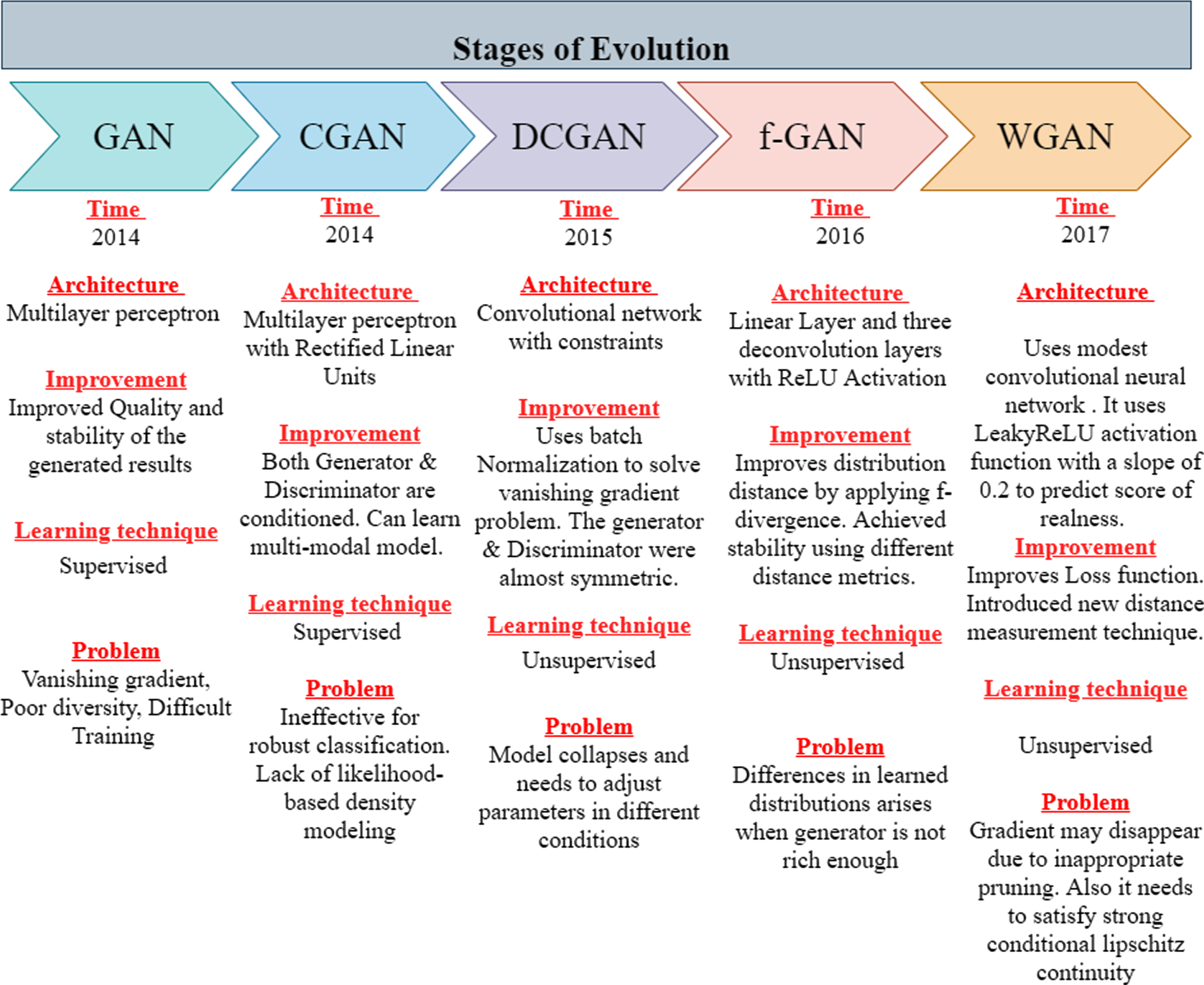
Despite many generative models available for different applications, generative models have shown low performance on certain image datasets. Some of the challenges include vanishing gradient, mode collapse, non-convergence, and problem with perspective [23]. Thus, researchers have proposed modifications and extensions of the existing GAN model such as CGAN [24], DCGAN [25], InfoGAN [26], ACGAN [27], WGAN [28], COVIDGAN [21], StyleGAN [29], and PGGAN [30] to address these problems. These problems have left researchers with another problem which is solving the conflict of choice when it comes to choosing the best GAN models for image augmentation. Each of the GAN models mentioned above has their pros and cons when applied to image data, as depicted in Fig. 6. Thus, in this study, we selected some of the most prominent generative models for image generation to compare and analyze their strengths and weakness using the COVID-19 CT-images and COVID-19 X-Ray images as our case study. The main contributions of this paper are:

1. Using some select Generative Adversarial Network Models to study how each COVID-19 image dataset reacts on the selected model.
2. Identifying the best candidate model for data augmentation among the selected algorithms to suit image augmentation when producing large datasets.
3. Illustrating how Visual Turing Test can be applied to the selected models to identify the best algorithm that generated the best images.

1.1Motivation

One of the obvious reasons that caused delay in the creation and development of COVID-19 vaccine and remedy was the lack of sufficient information (data) about the virus [10]. At some point, only a few hospitals and universities around the world (e.g., John Hopkins University [31]) had information about the virus. As such, it was very difficult to develop a cure. Notwithstanding, lack of data should not be an excuse that would halt the development of the cure. Thus, researchers kept looking for alternatives to close the gaps. One of the alternatives was to try every possible solution at hand. Hence, what motivated this study is the fact that data samples have to be made available for research and development. Finding the best tool to achieve this objective is very important, which is why this very study conducted a series of tests and evaluation so as to discover the best tool for data augmentation.

2Background of the study

This section provides the reader with an overview on COVID-19 and recent studies related to COVID-19, the COVID-19 datasets, image augmentation and its techniques.

2.1COVID-19 overview

In December of 2019, a cluster of viral pneumonia cases originated from a province in China, known as the Wuhan province. Experts in the medical domains believe that it was caused by a previously known virus called the 2019 Novel Coronavirus, which was later renamed by the WHO as Coronavirus disease 2019 (COVID-19) [32]. Coronaviruses are a large group of viruses; consisting of a code of genetic materials surrounded by an envelope-like protein spike (as shown in Fig. 1). This envelope-like protein spike gives the virus the look of a crown, and the word “crown” in Latin is means corona. Hence the name coronavirus gets its name. Moreover, there are different types of coronaviruses that cause respiratory and sometimes gastrointestinal diseases.

Fig. 1

Structure of the SARS-CoV-2 [33].

Previous respiratory disease can be traced from the regular flu to pneumonia. In most people, the symptoms tend to be mild. However, some types of coronavirus can cause severe disease. This includes the Severe Acute Respiratory Syndrome Coronavirus (SARS-CoV) first identified in China in 2003 [33] and the Middle East Respiratory Syndrome coronavirus (MERS-CoV), which was first identified in Saudi Arabia in 2012. Coronavirus Disease 2019 (COVID-19) caused by the Severe Acute Respiratory Syndrome Coronavirus Type 2 (SARS-CoV-2) was first identified in Wuhan, China. The disease was initially detected in a group of people with pneumonia who came in contact with seafood and certain types of birds in Wuhan’s market in China. The disease has since spread from sick to others, including family members and health care workers and is now spreading like wildfire in the community worldwide. A total of 218 countries and territories around the world have reported a total of 90,022,800 confirmed cases of the coronavirus and a death toll of 1,933,188 deaths [34].

Coronaviruses circulate among animals. These viruses can often be transmitted from animals such as Camel, Ducks, Bats, and Monkeys to humans through a process called spillover [35]. However, this could be due to a range of factors such as mutations in the virus or increase contact between humans and animals. For instance, MERS-CoV was transmitted from camels, SARS-CoV from Civet cats, and the carrier of the SARS-CoV-2 is not known. Majority of patients commonly start showing signs of five days after contacting wit SARs-CoV02, however, the incubation period of COVID-19 ranges from 2 to 14 days.

The exact means of how the virus is transmitted remains a mystery. Still, the general notion is that respiratory viruses are often transmitted via droplets created when an infected patient sneezes or coughs or through surfaces or anything that has been contaminated with the virus such as hands, door handles, cups, money notes, Automatic Teller Machines so on. Individuals at the risk of getting infected with the coronavirus are those in close contact with animals such as live animal market workers and those caring for those who got infected, such as family members or health care workers [34].

The symptoms of COVID-19 could be mild to severe. However, amongst the symptoms are fever, cough and shortness of breath. In more severe cases, there could be pneumonia, kidney failure, diarrhoea, and sudden death (Fig. 2). The death rate varies from one geographical area to another, although it keeps increasing since the time of its appearance. Preventive measures so far have been nothing other than standard hygiene measures such as avoiding close contact through social distancing, covering the nose and mouth when sneezing and coughing, using protective equipment such as face mask and face barriers, washing hands regularly with soap and water and the application of alcohol-based hand sanitisers [36].

Fig. 2

Common Symptoms for COVID-19. [39].

To diagnose and detect COVID-19 symptoms, researchers across the world have attempted to developed groundbreaking solutions using various techniques. Some of these techniques were purely medical in nature while others adopt technology-based approaches such as automated diagnosis systems and artificial intelligence. Some of these works include [37] where radiologists employ computer tomography with ensemble machine learning to classify clustered images of infected lungs. [38] suggested a deep learning method using convolutional neural Networks to design a framework that fuses the features extracted from X-ray and CT images before classification in an effort to ensure the accuracy of the detection. Their model achieved an accuracy of 99%. [6] goes to the next level when they concatenate two different transfer learning frameworks to classify CT-images and X-Ray images. The result of this study shows that the approach performed excellently by achieving 99.87% accuracy due to the concatenation technique that was adopted.

2.2COVID-19 CT and X-ray images

Image recognition and image processing have contributed to computer assisted diagnosis for early detection of cancer and other complicated diseases [37] and most recently COVID-19 and pneumonia related illnesses. The combination of transfer learning and ensemble architecture has proven effective in classifying clustered images of lung lobes. Transfer learning techniques have displayed a staggering performance and robustness when it comes to COVID-19 detection [6].

This study used two different sets of COVID-19 datasets, namely CT-Images and Chest X-ray images. CT images and chest X-ray images have proven to be very effective when it comes to diagnosis of diseases and on one hand detection and prediction of the diseases using diagnosis systems such as artificial intelligence supported systems [6, 38]. The first dataset is the Chest X-ray dataset used in [40] for classification. The dataset contains a total of 5941 chest X-ray images taken from 2839 patients. Out of the total number of images, 1203 were normal images, 45 were COVID-19 images, 660 were non-covid viral pneumonia, and 931 were bacterial pneumonia images. The dataset is suitable for the present study because it gives a 91.4% accuracy for two classes and 83.5% accuracy for four classes, making the dataset a potential candidate for data augmentation as it contains only 5941 image samples. This number is considerably low for training deep learning algorithms.

The second dataset is a dataset used in [41], and it contains about 4356 chest CT-scan images from different patients. A total of 1735 the CT images were taken from pneumonia patients while, 1325 were non-pneumonia patients. Lastly, the 1296 CT images were taken from COVID-19 patients. This dataset was previously used for classification. It gives a remarkable result, including 86% accuracy for bacterial pneumonia vs COVID-19 and 94% accuracy for heathy versus COVID-19 [34]. This is a perfect candidate for dataset regeneration because of its data distribution and its small sample size. Figures 3 and 4 illustrate the images samples from the two datasets.

Fig. 3

Sample examples from COVID-19 X-ray image dataset. (a) COVID-19 infected (b) Pneumonia infected (c) Bacterial pneumonia infected (d) Healthy. [40].

Fig. 4

Sample examples from COVID-19 CT image Dataset. (a) Healthy lung (b) COVID-19 infected lungs (c) Pneumonia infected lungs. [41].

2.3Image augmentation

Data augmentation is one of the milestone achievements in the field of artificial intelligence. It is one of the techniques used to improve the performance of trained models in machine learning [42]. Data augmentation gives data scientist the ability to create artificial instances data by making certain modifications to the existing data while retaining the original datasets’ characteristics [10]. Data augmentation increases and diversifies the training datasets by applying different data transformation techniques, especially when it comes to image datasets. Some of these augmentation techniques include flipping the image vertically or horizontally or zooming in and zooming out and scaling or at times adding Gaussian noise to distort high-frequency features of the image as illustrated in Table 1.

Table 1

Image augmentation techniques tested on Ct-images

Technique	Original vs Synthesized Images	Description
Cropping		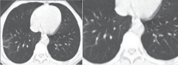Cropping images are used for images with mixed height and width dimensions where the central patch of an image gets cropped [10].
Colour Space		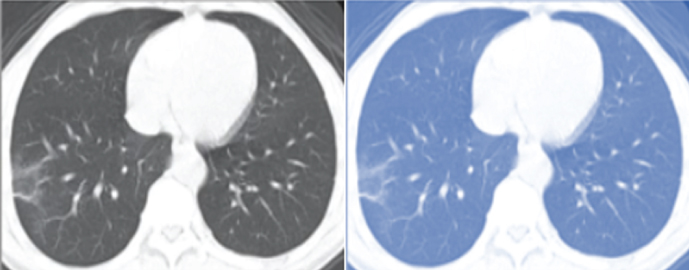The digital image is encoded as a tensor of the dimension (height×width×colour channels). Carrying out augmentations in colour channels space is an effective strategy. The isolation of a single colour or channels like R, G, or B is a simple colour augmentation [43].
Flipping		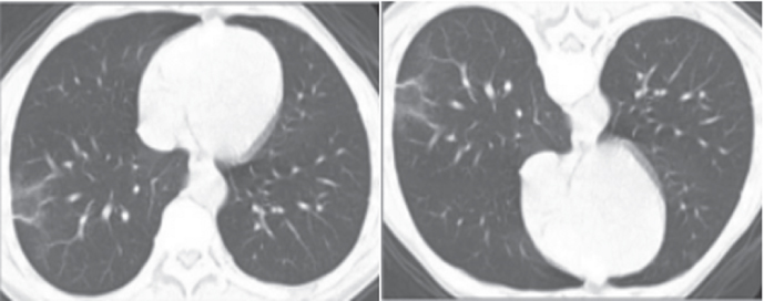Flipping horizontal axis is practiced more than the vertical axis flipping. It is among the simplest augmentation techniques that can be practiced, it has been found useful on datasets like ImageNet and CIFAR-10 [27].
Kernel Filters		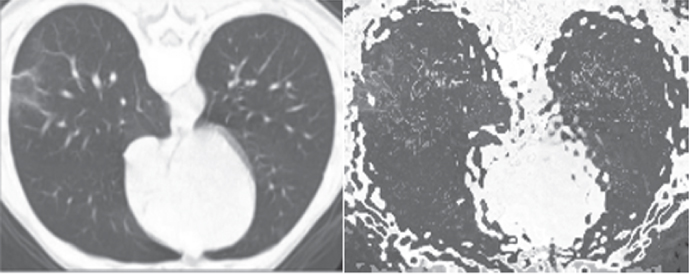It involves sliding an n×n matrix across an image using a Gaussian blur filter that produces a blurrier image or a high vertical or horizontal edge filter that produces a sharper image along edges [10].
Mixing Images		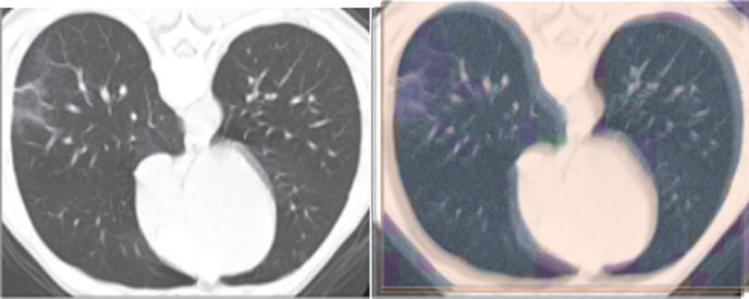Mixing images by taking the mean of these images’ pixel values is an augmentation strategy that is seen as counterintuitive. The images produced do not show any significant transformation to the human eye [44].
Noise Injection		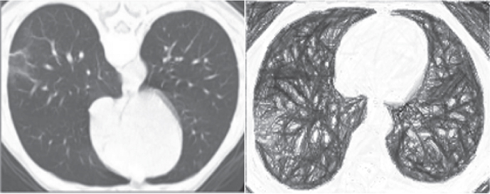Noise injection is a technique that employs the injection of matrix that has random values which are normally generated from a Gaussian distribution.
Rotation		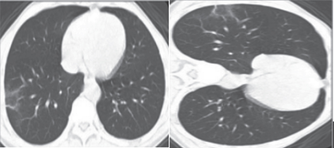This is achieved by rotating an image towards the left or right to an angle between 1° and 359°. The safety of rotation augmentations solely depends on the rotation degree parameter.
Random erasing		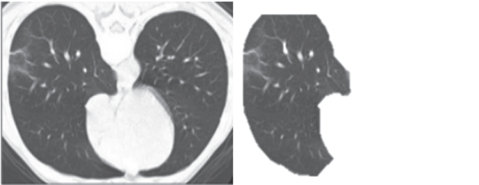Random erasing is meant for solving the problem of image recognition due to blurriness in some part of an object (occlusion). Random erasing prevents the occlusion by enforcing the model to identify more descriptive features of an image and prevents the image from fitting into some visual features in an image
Translation		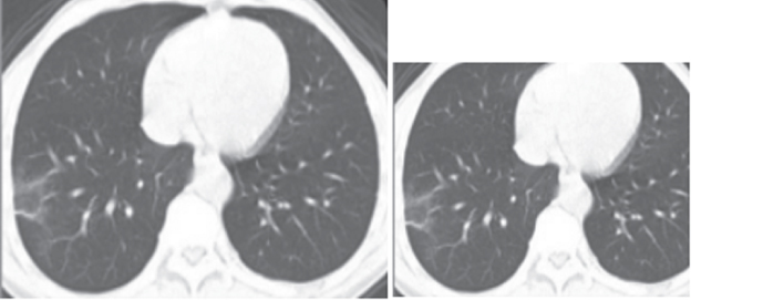This involves shifting images to the left, right, up or down to avoid positional bias in the image data.

Data augmentation has also proven to be handy when it comes to reducing overfitting. Overfitting is when there is an error in a model due to functions corresponding too closely to one particular side of the data, also known as imbalance in data distribution. One technique that can be applied to reduce overfitting is to add more datasets to the training data by augmenting the existing data to create a more balanced data for better performance and training [10].

3Generative adversarial networks

Generative Adversarial Networks (GANs) are described as unsupervised neural network models that generate synthetic data after taking a given input data [12]. It is important to acknowledge that the GAN was first introduced into the Deep Learning domain by a group of experts headed by Ian Goodfellow in their 2014 paper titled Generative Adversarial Nets [45]. Since then, lots of research have been done using GAN for different applications and for solving different domain problem. It has been used in different activities that involve computer vision, classification and data transformation. Generative models have generally been grouped into two, one being the deep learning models comprising the autoencoder (AE) [27], GANs, and its derivative models. The second group is the traditional generation algorithm that is categorized based on machine learning. It involves Hidden Markov Model (HMM) [26], Naïve Bayes Model (NBM) [25], and Boltzmann Machine (RBM) [24]. GAN can be described as a form of generative model that is concerned with generating target data through the use of latent variables. The model involves game training that is carried out between a Generator and Discriminator, where random variables that are known to obey Gauss distribution generate target variables that have a real data distribution. GANs are relatively simpler, more functional, and possess more application scenario than the traditional machine learning algorithm. It also has a greater performance as compared to the traditional algorithms when dealing with larger datasets.

Ian Goodfellow describes the generative model as an analogous to a group of counterfeiters who are trying to produce fake currency and spend it without being detected. Meanwhile, he describes the discriminant model as an analogous law enforcement officer trying to detect counterfeit money when out for use [45]. In essence, we can say that the generative model finds a way to generate interesting information from the given values. Simultaneously, the Discriminator tries to recognize the generated information from the original input [46]. For learning to occur over the generator’s distribution p_g over data x, input noise variables p_z (z), are defined. Next, a mapping to data space is represented as G (z ; θ_g) where G s a distinguishable function that is often represented by a multilayer perceptron alongside parameters θ_g. More so, another multilayer perceptron D (x ; θ_d) is defined to output a single scalar. Also, D (x) denotes the probability that the value of x came from the original data instead of p_g. Here, D is trained to increase or maximize the probability of giving the accurate or correct label to training data and the samples from G. In the end, G is trained to minimize log(1 - D (G (z))) [45].

3.1GAN evolution

The GANs’ evolution can be briefly described in the following stages, as illustrated in Fig. 5. The most important parts of each stage are DCGAN and WGAN, as an important generative model is represented in DCGAN. This model has an easier operation mode than the other developed models before it, and it is more stable. The development of WGAN has upgraded the level of GAN, as it can get samples that are of relatively high quality [29]. Various GAN models were produced sequentially and employed in different computer vision fields based on the requirements of various tasks and scenarios.

Fig. 5

GAN stages of evolution.

Also, it has great performance in other important fields that include art, security encryption and even medical fields. Images that have high fidelity and low gap were first generated by BigGAN [47], leaps and bounds were used to enhance its correctness, which was an important event in the history of the development of GAN. StyleGAN [29] is also a great advancement in GAN’s study. It has brought about a new record in tasks involving face generation. The style transfer, otherwise called style mixing is the fundamental part of the algorithm. Other than generating faces, it can generate bedrooms, cars, and other high-quality images. In the cases of face ageing and other industries, Age-cGAN [48] is another vital model applicable in cases involving face ageing and even in some industries to find missing children cross-age face recognition or entertainment.

Nonetheless, a study conducted on GANs has revealed that in addition to the fast development in image and video processing, it can as well function in speech processing, text processing, and signal processing fields which include speech super-resolution, text-synthesized images, ECG, and EEG signal recognition [43].

3.1GAN architecture

The GAN architecture represents the topological structure that made up what we describe as the generative adversarial networks. Like many algorithms out there, GAN also has its complex architecture that comprises two basic elements: the generator model and the discriminator model as highlighted previously. Both the former and the latter can be implemented using any neural network such as Deep Neural Network, a Convolutional Neural Network or a Recurrent Neural Network. However, the Discriminator uses a fully well-connected layers with one or more classifiers at the end [49].

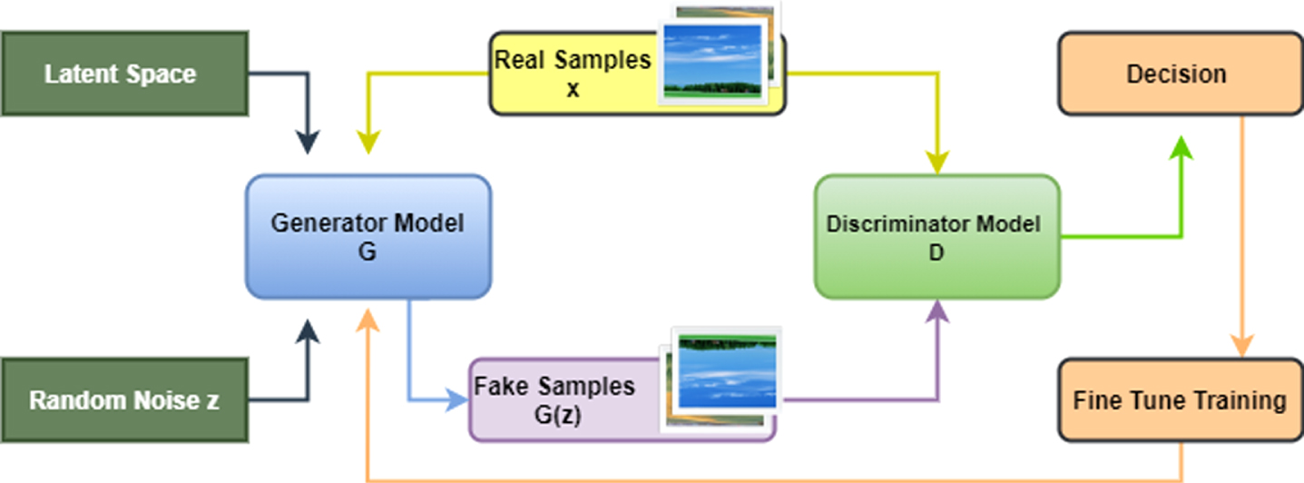
Furthermore, the Generator and Discriminator start to train alongside each other. The generator aims at producing a set of data that would look almost exactly to a real one. The Discriminator’s role is to be able to detect the difference between the newly generated data from the real or original data. Normally, the Discriminator has to train for a few moments before starting the adversarial training. As illustrated in Fig. 6, the generator is given some input samples. It learns the features and generates fake samples based on the learned features. The original as well as the fake samples are forwarded to the Discriminator. The Discriminator uses that forwarded data to predict the probability of the samples being fake or original. Both the Discriminator and the Generator compete against one another using the game theory concept (“Game theory is the study of models of strategic interaction among rational decision-makers” [50]). At the same time, vectors of noise are given along with the training samples to the generator. However, the generator learns the features in the samples and then generates data samples which match the properties of the given input.

Fig. 6

Initial GAN architecture.

3.1.1The generator

A differentiable function, G is used to represent the generator, which deals with a collection of random variables denoted by z from an initial distribution, these are then mapped to a pseudo-sample distribution denoted by G(z), via a neural network. This process is referred to as upsampling process [51]. A random variable, or a random variable in latent space, referred to as Gaussian noise is commonly used by input z. The G and D parameters are repeatedly updating while the training of GAN progresses. The D parameters become fixed while G is trained. The data it generates is shown to be of a false nature, hence input into D. The error is therefore estimated between the sample label and outputs of D(G(z)) which is the Discriminator Between the output of the discriminator D(G(z)), the parameters of G is updated by an error backpropagation algorithm. G establishes some limitations on input variables that can be in input to both the first and last layers. Nonetheless, noise can be inserted through hidden layers, using summation product. GAN imposes no constraint on the input dimension of z that normally happens to be a 100-dimensional vector. Moreover, as feedback is passed via the Discriminator will reinstall the gradients to get the G and D parameters updated, G is expected to be easily differentiated. The Generator loss can be computed as follows:

(1)

LGANG=-Ex∼pz[log(D(G(z)))]

3.1.2The discriminator

The goal of discriminator D is to determine whether the input is from a real sample and provides a feedback mechanism that refines weight parameters of G. When the input is real sample x, the output of D approaches to 1. Otherwise, the output of D approaches to 0. When the Discriminator is trained, the G is fixed. D obtains the positive sample x from the real dataset and the negative sample G(z) generated by the generator. Both of them are input into D, and the output of D and sample labels are used to calculate the error. Finally, the error backpropagation algorithm is used to update the parameters of the Discriminator. The Discriminator can be illustrated in the following quotation:

(2)

LGAND=-Ex∼pdata[log(D(x))]-Ez∼pz[log(1-D(G(z)))]

3.1.3The loss function

GAN’s loss function depends on the minimax of two gamers that involves two neural networks that compete with the framework of a zero-sum game [35]. It is expected of the Discriminator to differentiate between the input data and the true one, then use the backpropagation algorithm in optimizing the weight of the network model. X and θ^(D) are the input parameters of discrimination while the loss function of the Discriminator is given by the equation below:

(3)

V(D,θ(D))=-Ex∼Pr(x)[logD(x)]-Ez∼pg(z)[log(1-D(z))].

Among these, P_r and P_g denote the data distributions for actual samples and false samples generated by the generator, respectively. Z and θ^(G) are the input parameters of the generator, and the loss function is given by the equation below:

(4)

V(G,θ(G))=-Ez∼pg[-log(D(G(z)))].

The weight of θ^(D) is optimized by a discriminator, and that of θ^(G) is optimized by a generator via loss function. When the discriminators and generators are being trained the model parameters of the two remains the same. And the training continues till the two network structures attain a Nash equilibrium [36]. Two distinct types of network structures are being trained by the GAN model using an adversarial model; the last objective function of GAN model is given by the equation below:

(5)

minGmaxVD(G,D)=minGmaxEDx∼pr(x)[logD(x)]+Ez∼pg(z)[log(1-D(G(z)))]

4GAN models for image augmentation

The GAN is a great algorithm, and it has dramatically changed the paradigm of image augmentation and image transformation over the years since its release in 2014. It has significantly gained statistical advantages over its pairs such as RBM, HMM, GMM, and Autoencoder. However, the framework suffers from a great deal of issues such as vanishing gradient, poor diversity and difficulty to train in certain conditions. A lot of efforts have been made over the last few years to obtain a better representation of GAN through different optimization techniques by proposing new architectures with improved and stabled structure. Some of these models are described below:

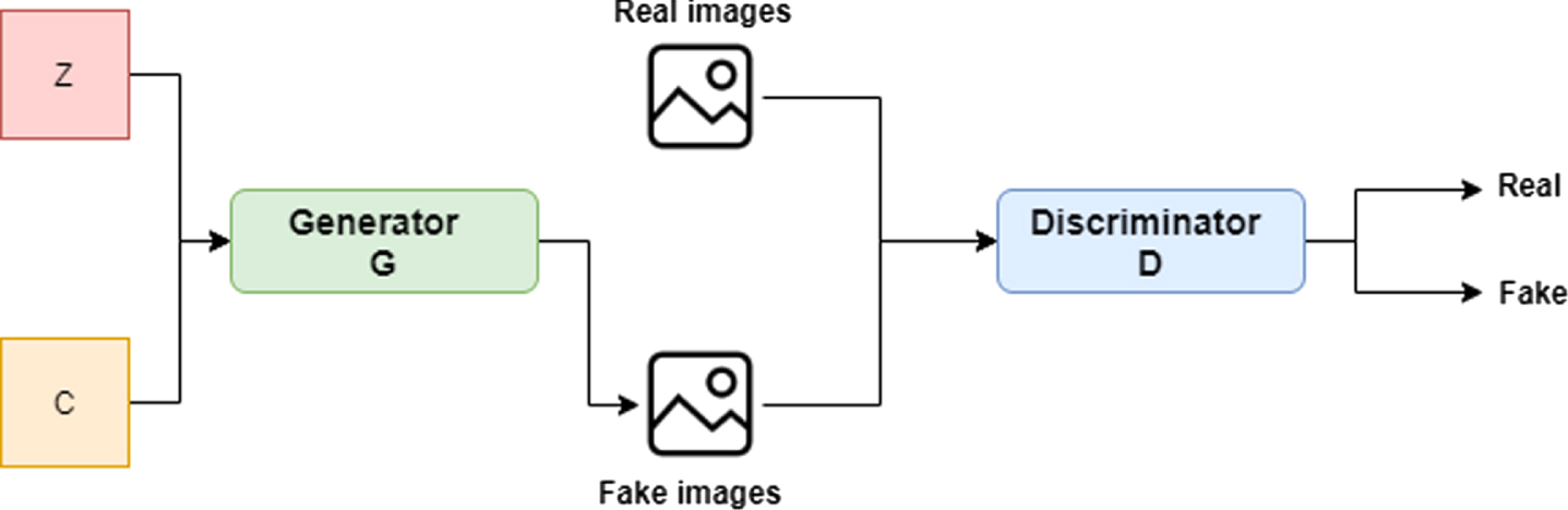
4.1Conditional Generative Adversarial Network (CGAN)

CGAN is a modified GAN model propounded by Mehdi Mirza and Simon Osindero in their 2014 paper titled “Conditional Generative Adversarial Nets” [24]. Contrary to the original GAN, CGAN is a model that employs a supervised method of enhancing the ability to control generated results. In CGAN, the random noise z and the category label c are assumed to be the inputs of the generator and the generated fake/real sample, category label is used as the discriminator input, so as to comprehend the relationships between images and labels. To guide the data generation, a condition variable, y is introduced to the modelling, and conditions are included in the model with n extra information y as seen in Fig. 7.

Fig. 7

CGAN architecture.

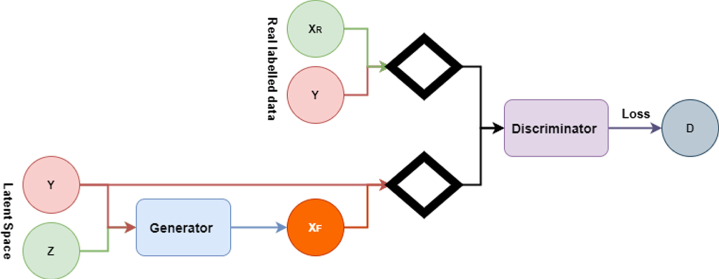
In a broader sense, the generator model takes as input noise p_z (z), and y combined in a joint hidden layer. While the discriminator model takes x and y as input as well as a discriminative function in the case of a multilayer perceptron. The architecture can be expressed as:

(6)

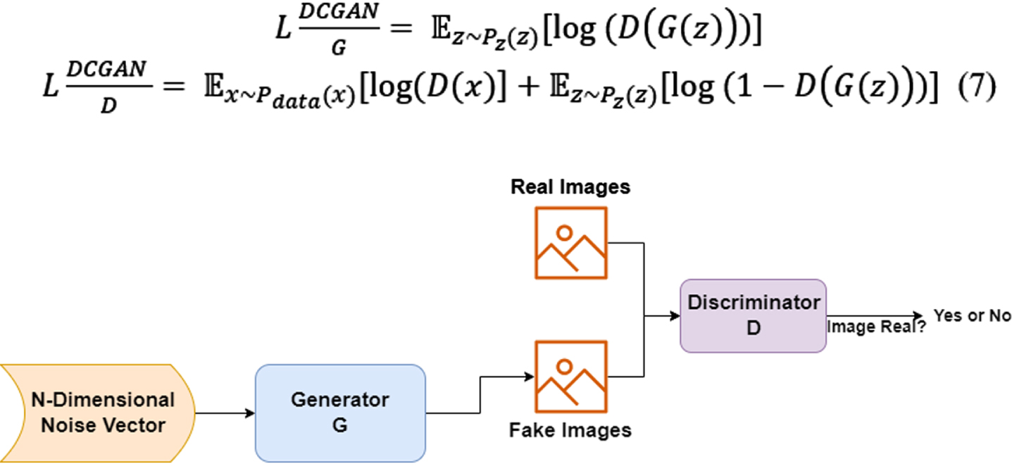
minGmaxDV(D,G)=Ex∼pdata(x)[logD(x|y)]+Ez∼pz(z)[log(1-D)(G(z|y))]

4.2Deep Convolutional Generative Adversarial Networks (DCGAN)

After a year of publication of the GAN paper, the researchers realized that the model was not stable and that a large amount of training on it was needed. Radford et al. [25] brought forward an advanced version of GAN architecture in the year 2015 and it was called DCGAN Fig. 8. The authors of this version used deep convolutional networks (CNNs) in enhancing the architecture of the original GAN. Until now, the DCGAN’s network structure has a wide coverage and is considered the best GAN architecture and a significant event in the history of GAN. In the DGGAN setup, the convolutional layer is used almost entirely by DCGAN, contrary to the fully connected layer that is being used by the original GAN. The Discriminator is roughly proportional to the generator; the whole network lacks pooling layers and up-sampling layers. Batch Normalization Algorithm is applied by the DCGAN in problem-solving that involves vanishing gradient. Both the generator model and the discriminator model are presented with their loss function below:

(7)

LDCGANG=Ez∼pz(z)[log(D(G(z)))]LDCGAND=Ex∼pdata(x)[log(D(x))]+Ez∼pz(x)[log(1-D(G(z)))]

Fig. 8

DCGAN architecture.

4.3f-GAN

The original GAN has an objective function, which is to minimize the JS divergence that exists between two distributions. The JS divergence is among the many methods that can be adapted to measure the distance between two given distributions. Various objective functions can arise from defining various distance metrics. [52] employed the use of f-divergence in GAN (f-GAN) to train generative neural samplers. The f-divergence is a function Df(P||Q) used to measure the variation between two probability distributions given as P and Q as illustrated in the equation below:

(8)

Df(p,q)=Ex∼q[f(p(x)q(x))]

According to the structure of f-divergence, f-GAN generalizes other divergences in such a way that the corresponding GAN objective can be obtained for a particular divergence. However, to initiate the f-GAN objective, we adopt two commonly used techniques from convex optimization, i.e. the Fenchel conjugate as well as duality [52]. In essence, a lower bound to the f-divergence is collected through its Fenchel conjugate as in the below equation:

(9)

Df(p,q)⩾supT∈T(Ex∼p[T(x)]-Ex∼q[f*(T(x))])

Many similar divergences like [53] KL-divergence, Hellinger distance, and total variation distance, are exceptional cases of f-divergence concurrent to a specific choice of various distance metrics distributions were applied to GAN training stability in order to enhance it.

4.4Wasserstein Generative Adversarial Networks (WGAN)

WGAN principally upgraded GAN from the loss function viewpoint. Theoretically, it highlighted the cause of the instability of GAN training, which is, the cross-entropy is found to be inappropriate for measuring the distance between distributions that have disjoint parts [54]. The WGAN put forward another approach to be used in measuring distance, which is the Earth Moving Distance, otherwise called Wasserstein distance or optimal transmission distance. It describes the least transmission quality that can convert the probability distribution, q to probability quality, p (known as the probability density in discrete cases) [28]. Notation (10) was suggested to measure the distance between real images and fake images:

(10)

W(Pr,Pθ)=infγ∼Π(pr,pg)E(x,y)∼γ[∥x-y∥]γ∼Π(pr,pg)

Based on the above, Π (p_r, p_g) is the representative of all possible joint distributions that are combined by both p_r and, p_g. The Wasserstein distance is better than both the KL and JS divergence in that, it can reflect the distance between two distributions despite being disjoint. Both the theoretical derivation and interpretation of WGAN are not straightforward. The authors of WGAN [28] declared that applying Wasserstein distances is expected to meet a strong continuity condition which is the Lipchitz continuity. See Fig. 9 WGAN architecture below:

Fig. 9

WGAN architecture.

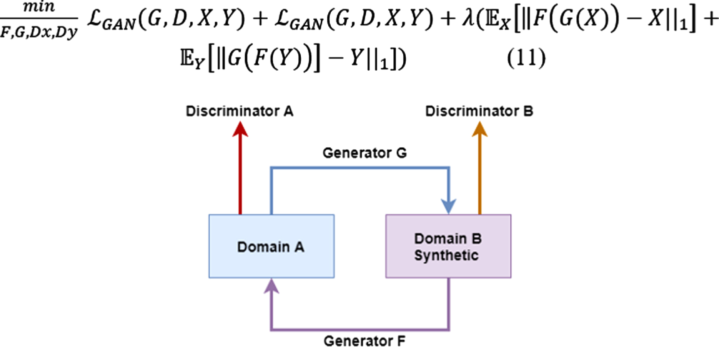
4.5CycleGAN

CycleGAN is an unsupervised GAN type that enables image to image operations in a circular fashion such as image translation as illustrated in Fig. 10. Jun-Yan Zhu, Taesung Park, Phillip Isola, and Alexei A. Efros, were the first to propound the CycleGAN. Two adversarial mappings make up the architecture as follows: G:X->X. G is in charge of generating outputs from X, while the Y determines whether they are real or false. F, on the other hand, is in charge of generating outputs from Y while X determines whether they are real or false. However, GAN ensures that the cyclic loss that is experienced while input is being translated from X to Y and all over again is minimal. CycleGAN evokes a property described as cycle consistency which denotes that if we can traverses X to Y through G, hence we should likewise be able to traverses Y to X through F. The loss function is expressed as follows:

(11)

minF,G,Dx,DyLGAN(G,D,X,Y)+LGAN(G,D,X,Y)+λ(EX[∥F(G(X))-X∥1]+EY[∥G(F(Y))-Y∥1])

Fig. 10

CycleGAN architecture.

5Experiments

This section discusses the setup environment and how the experiments were conducted, and the evaluation techniques used to measure the algorithms’ performance.

5.1Experimental setup

The experiment was conducted on a 9th Generation Core i7 Intel Machine with GTX 2060 ti 6GB GPU support. We developed and trained our models in a TensorFlow and Keras environment using two unique datasets, namely Chest X-ray dataset from [17] and chest CT-scan images from [18]. Fifty image samples were randomly selected from each dataset and were reshuffled for processing. All the images were of 28x28 pixels and a greyscale value assigned to each pixel.

This study aims to generate realistic-looking synthesized CT scan images and X-Ray images to serve as a representative of the original samples. We compared the generated sample images using different discriminators. By combining the different GAN architectures, visual attributes of reconstructed images were created. The five architectures used are regular GAN models including CGAN, DCGAN, f-GAN, WGAN and CycleGAN as illustrated in Fig. 11. We compare each model’s outcome in terms of how their different GAN architecture plays a role in synthesizing the newly generated samples. The generators and discriminators are the same as the convolutional neural networks we found in many studies. In all the training sessions, we used optimizers such as Adam’s optimizer [55] to minimize the loss functions using a learning rate of 10-5 and a batch size of 64. For the Adam’s optimizer to work perfectly, we applied 0.5 for β₁ likewise 0.9 for β₂ when training models like WGAN and CGAN. All five models were trained in 60 epochs in all the two datasets. This is because gradient descent apply iterative algorithms [51].

Fig. 11

Comparison of five different GAN models on two different datasets.

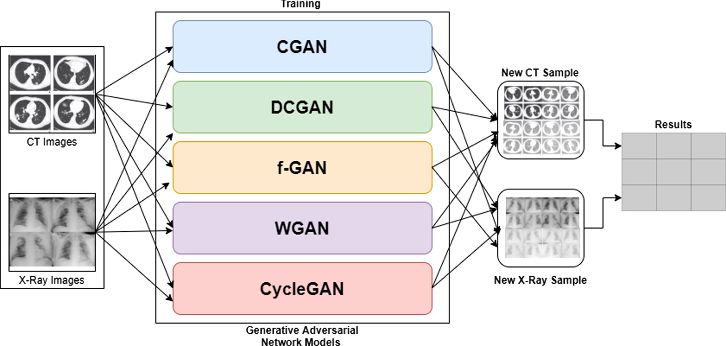
For the implementation part, we divided tasks into three: The first task was to write the basic functions to generate real data distribution of each dataset. Secondly, we wrote the lines for the Generator model and then the Discriminator model. Furthermore, lastly, we wrote the lines to be used by the data and the networks to carry out the training in an adversarial manner. For each model used, we started with vectorization process to ensure that all images are of the same size. Depending on which model is to be run, some models like DCGAN have to run using convolutional and deconvolutional neural networks for the Generator and the Discriminator. We started by using a feedforward neural network to initialize each generator, and the input assigned to the network is random noise. At the last layer of each network, shape matching the input datasets’ dimension is expected as the outcome. These tasks’ primary objective is to learn how each GAN model trains the data and regenerate the new set of data on each GAN model.

5.1.1Evaluation metrics

To evaluate the different GAN models’ performance, namely, CGAN, DCGAN, f-GAN, WGAN and CycleGAN, on the two datasets, this study employs two commonly used evaluation technique, i.e., qualitative and quantitative. Qualitative evaluation technique relies on human experts to observe the produced images and make their assessment based on the quality of the images using a technique called Visual Turing test as proposed by Geman et al., in their paper [56]. According to the author, Visual Turing test “Is an operator-assisted device that produces a stochastic sequence of binary questions from a given test image”. In essence, the engine creates an array of questions that seem to have unpredictable answers. Here, the task of a human operator is to supply the correct answers to the posed questions or reject it if it seems ambiguous. Visual Turing test basically has four types of questions which must return an answer or term the questions scenario as ambiguous (see Table 2):

Table 2

Visual turning test possible questions

Nature of Question	Questions	Notation
Existence	“Is there an instance of an object of type t with attributes A partially visible in region w that was not previously instantiated?”	Q_exist
Uniqueness	“Is there a unique instance of an object of type t with attributes A partially visible in region w that was not previously instantiated?”	Q_uniq
Attribute	“{’Does object o_t have attribute a?’, ‘Does object o_t have attribute a₁ or attribute a₂?’, ‘Does object o_t have attribute a₁ and attribute a₂?’}”	Q_att(o_t)
Relationship	“Does object o_t have relationship r with object o_t’?”	Q_rel (o_t, o_t′)

To fulfil the VTT requirements, a medical expert was asked to differentiate between the original images and the synthesized images in random order 80%. On the other hand, quantitative evaluation is also applied to abolish any possibility of doubt. This technique relies on calculating specific numerical scores used to assess the quality of the synthesized data. Some of these quantitative approaches include average Log-likelihood, Coverage metric, inception score, Fréchet Inception Distance, Boundary Distortion, Precision, Recall and F1 score and many others.

In this study, we used Fréchet Inception Distance (FID) for the evaluation of the generated outcomes. The FID was proposed by [57] in their study titled GANs Trained by a Two Time-Scale Update Rule Converge to a Local Nash Equilibrium. The FID suggested that to justify the quality of generated data samples; first, they have to be embedded into a feature space allocated by an inception net. Second, displaying the embedded layer as a multivariate Gaussian, then the covariance and the mean are estimated for both generated image samples and the original image samples [57]. FID is represented as follows:

FID(x,g)=||μx-μg||22+Tr(Σx+Σg-2(ΣxΣg)12) , where (μ_x, Σ_x) and (μ_g, Σ_g) are the covariance and the mean of the image samples embeddings from the sample and model distribution respectively.

6Results and discussion

As highlighted above, the experiment was conducted on two unique datasets, namely the CT-Images and X-Ray Images for both COVID-19 infected and non-infected victims. As mentioned in Section VI, this study utilizes two evaluation approach qualitative and quantitative approaches. In terms of the quality of the synthesized images, results are judged based on human visual observation using visual Turing test. In this study, a medical expert was shown 50 real images and 50 synthesized images generated by the models, as seen in Table 3. The images were later selected at random and turned over to the medical expert for analysis. Images that scored > 50% indicate a superior outcome. The results are presented in Table 4.

Table 3

Comparing different CT-image datasets and X-Ray datasets results based on each model’s performance. On the left are the original images before augmentation. On the right are the synthesized images produced from the originals

Datasets	Models	Original images	Synthesized images
CT-Images	CGAN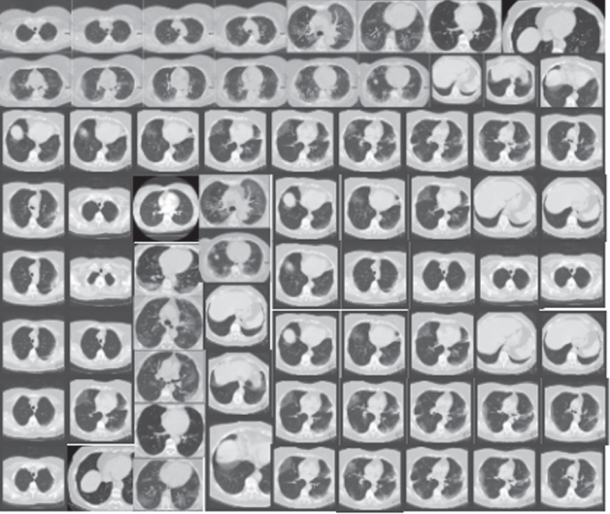
	DCGAN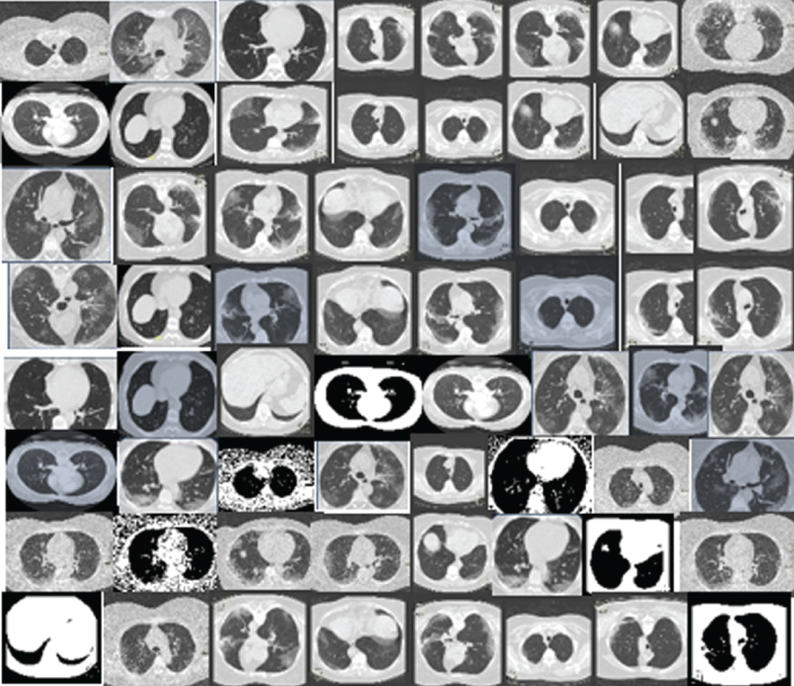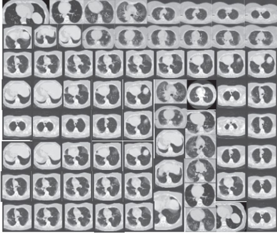
	F-GAN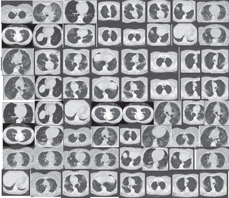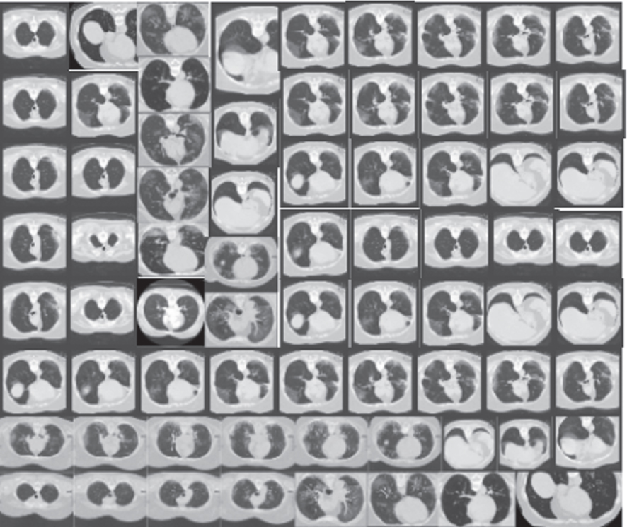
	WGAN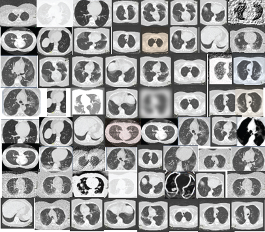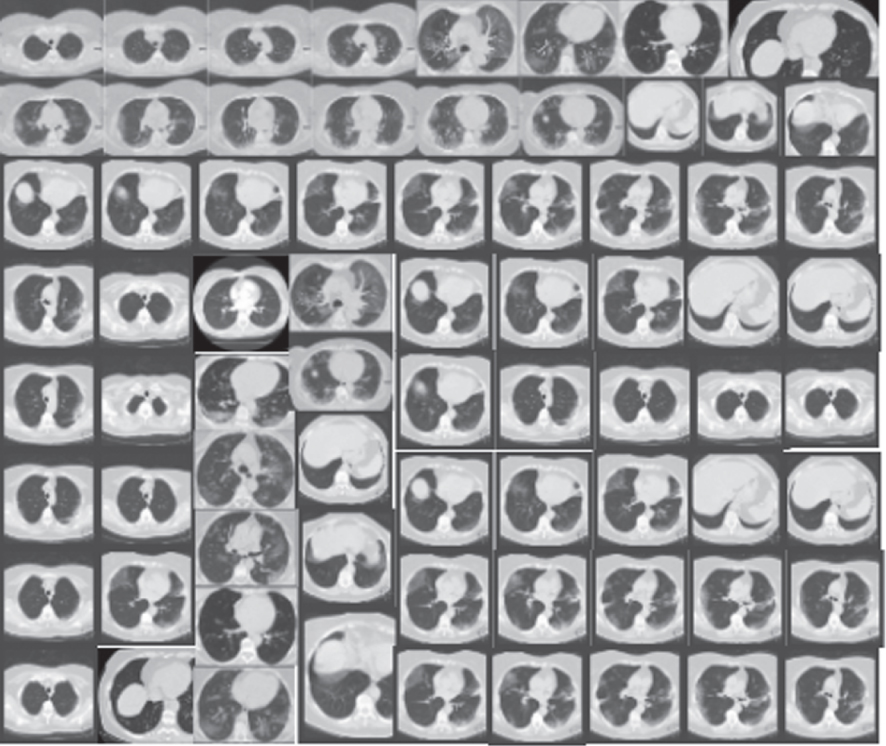
	CycleGAN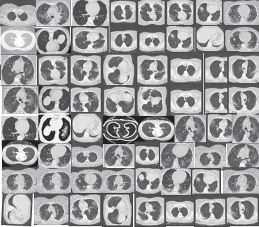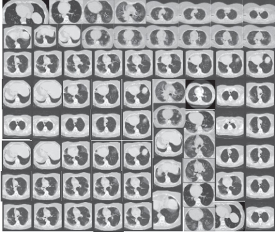
X-Ray Images	CGAN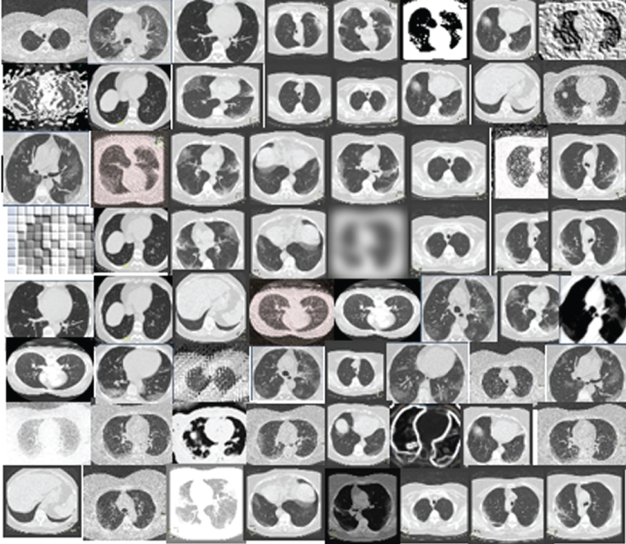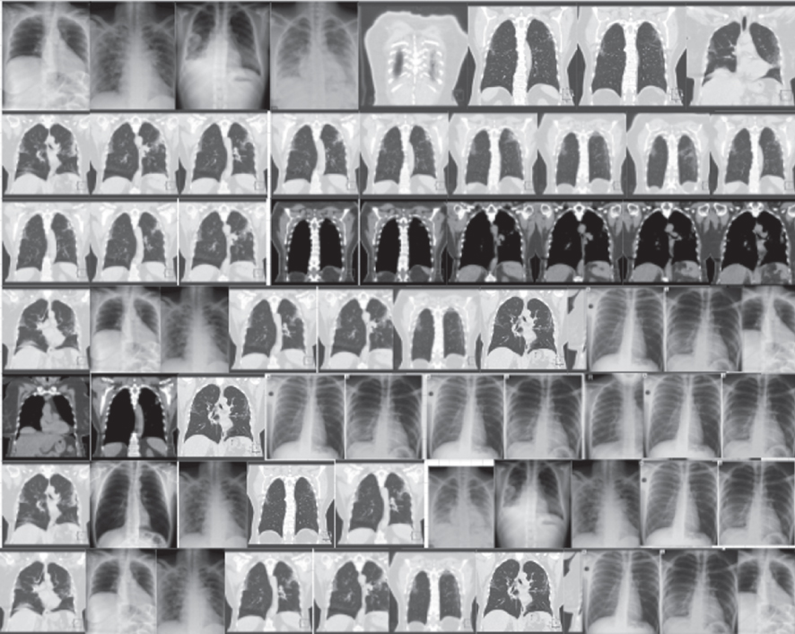
	DCGAN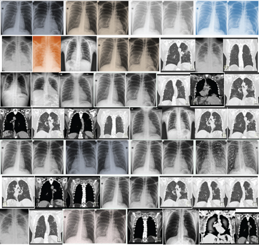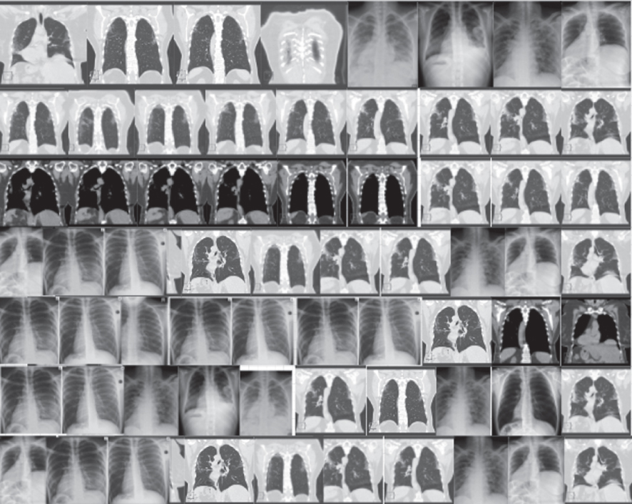
	F-GAN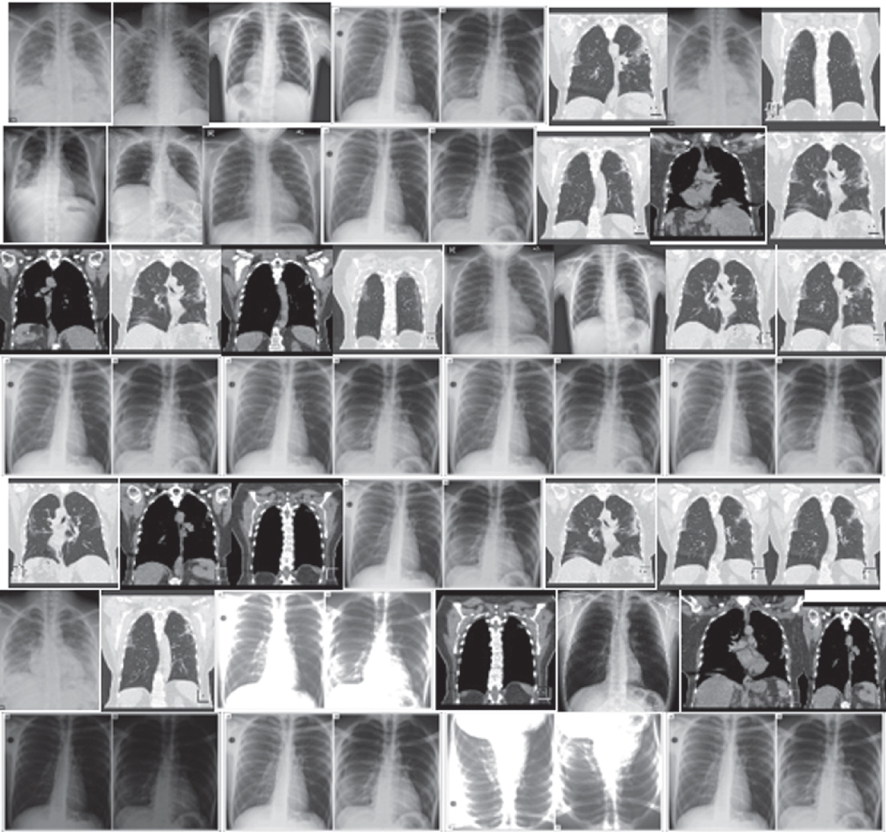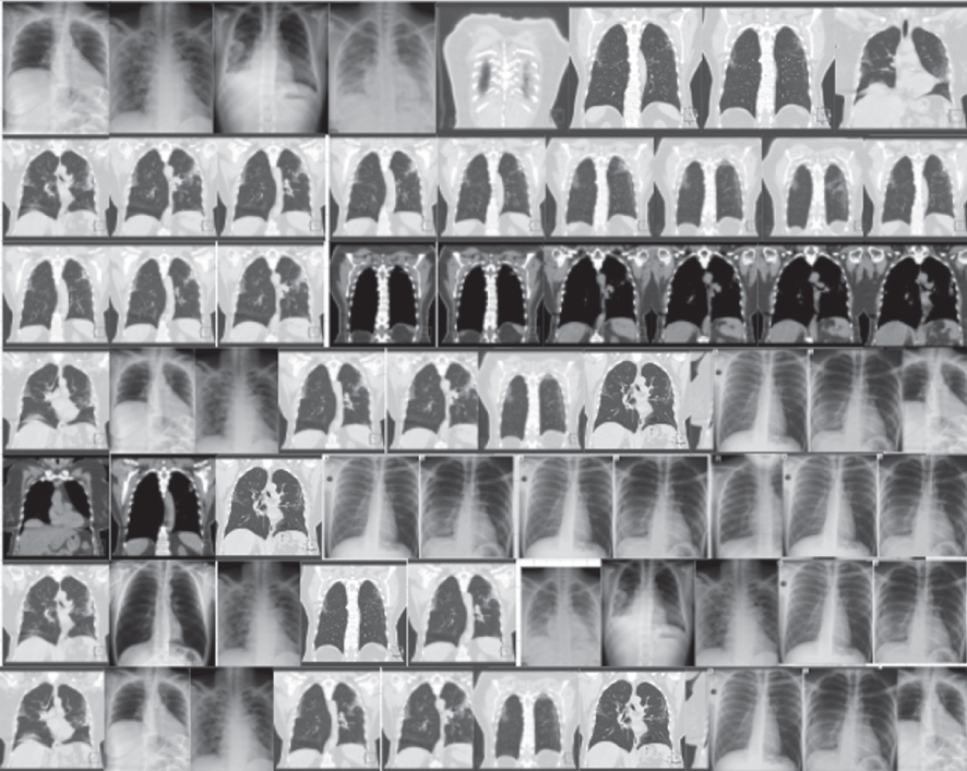
	WGAN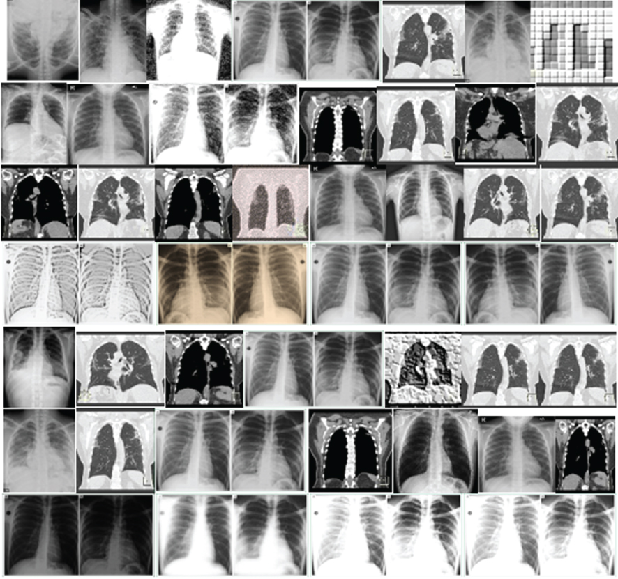
	CycleGAN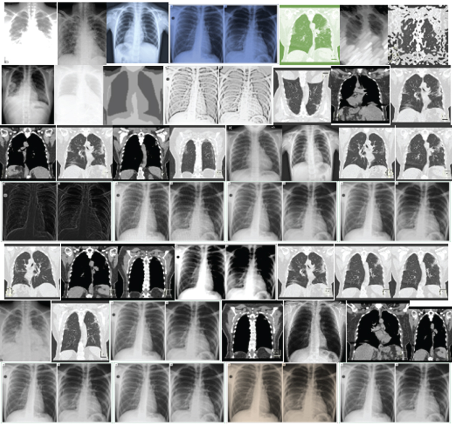

Table 4

Results from Visual Turing Test by a physician for differentiating real vs synthesized images. Note that images which scored 50% and above indicate good result as agreed in previous studies [58]

Dataset	GANs Model	Real as Real	Real as Synth	Synth as Real	Synth as Synth	Accuracy (%)
CT-Images	CGAN	26	24	7	40	71
	DCGAN	25	25	4	45	73
	F-GAN	22	28	7	41	66
	WGAN	13	34	9	44	54
	CycleGAN	29	17	10	42	80
X-Ray Images	CGAN	25	22	5	45	70
	DCGAN	25	24	4	46	72
	F-GAN	23	25	7	44	60
	WGAN	15	30	9	40	59
	CycleGAN	34	15	8	38	77

6.1Visual turing test results

Based on the results seen in Table 4, it quite tough for a human expert to accurately distinguish the differences due to lower resolution or loss in the appearance. However, distinguishing DCGAN is a lot easier compared to the rest. CycleGAN gives tough time. It confused the expert into thinking if they have any difference between DCGAN and CycleGAN. Finally, CycleGAN comes on top with a promising result of 80% in CT image dataset and 77% in the X-Ray image dataset.

It is also important to note that CGAN can generate more realistic multi-sequence CT-Images that show promising results and have not confused experts in distinguishing from the real ones. In general, WGAN displays a low performance (with 54% for CT images and 59% for X-Ray images) as well as mode collapse when compared with others in terms of intensity. Our study indicates that human experts are reliable evaluation tools, but for a more objective and unbiased evaluation, we must use other computational evaluation techniques to assess our models for efficiency and performance.

6.2Fréchet inception distance measure

As clearly mentioned in Section VI, FID allows us to measure the quality of the generated samples as they are embedded into a feature space denoted by a certain layer of inception network [59]. However, this gives us a continuous multivariate Gaussian embedded layer. The mean and the covariance are estimated for both real data and the synthesized data. The FID distance utilized to measure the quality of the synthesized samples, as illustrated below:

(12)

FID(x,g)=||μx-μg||22+Tr(Σx+Σg-2(ΣxΣg)12)

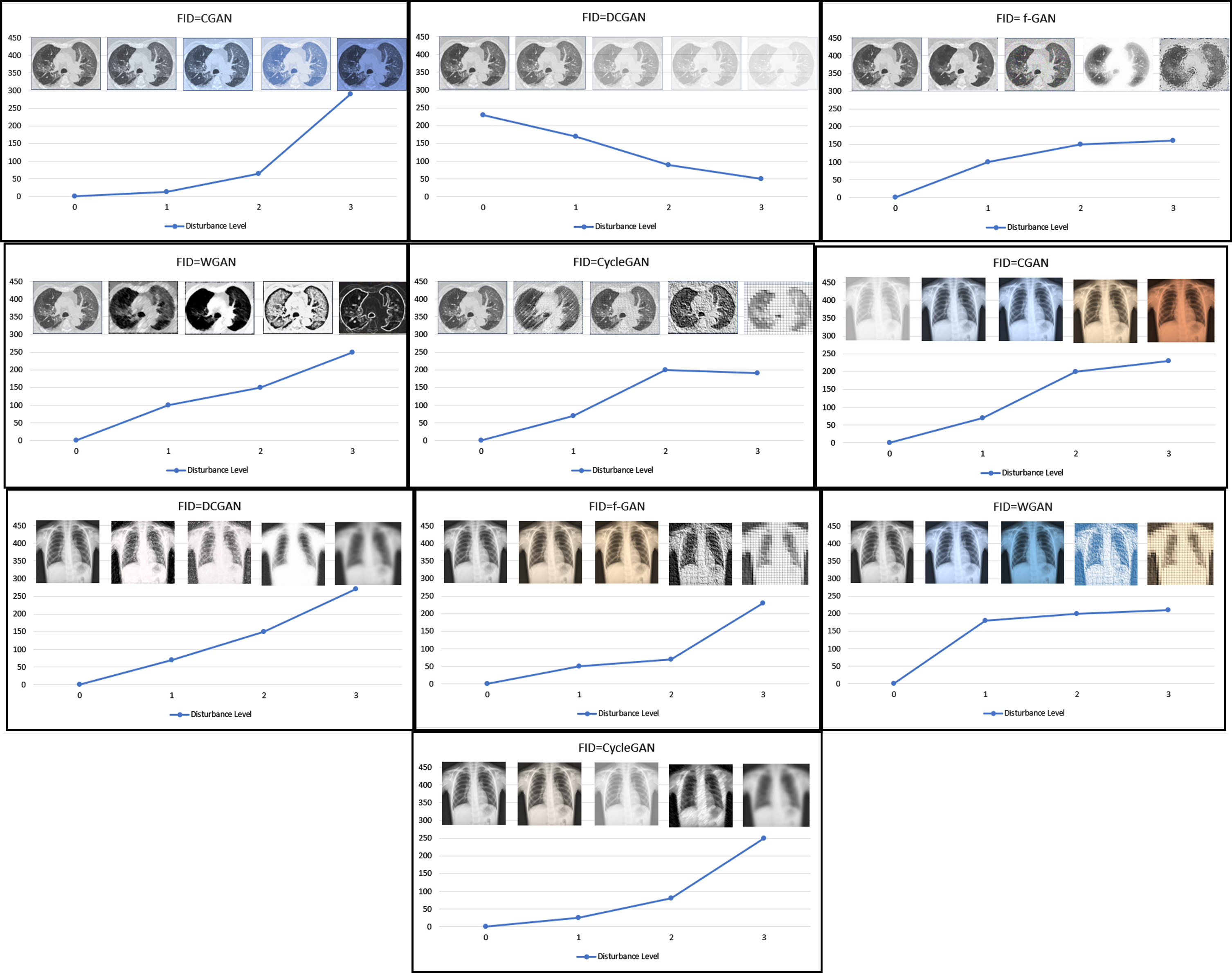
Figure 12 indicate that FID is a very sensitive evaluation measure. It shows the distortions of various images. Various GAN models demonstrated different properties, from the left to the right and top to bottom of the chart. It is apparent that Gaussian noise has affected the synthesis process in some of the images. The noise increases and gives a more Gaussian blur in some of the images. Based on the image, the (μ_x, Σ_x), and (μ_g, Σ_g) are the covariance and mean of the generated samples and model distribution. Here, lower FID denotes smaller distances between the generated samples and the original samples. It is apparent that FID does well in discriminating the new samples from the original samples.

Fig. 12

FID results showing distortion levels at various phases.

To answer the key question, i.e. which model performs the best among the five models, namely CGAN, DCGAN, f-GAN, WGAN and CycleGAN, is answered in Table 5. In terms of quality of the images generated by each model, CycleGAN shows the high convergence and therefore generated high quality and clearer samples on both datasets than CGAN, DCGAN, f-GAN, and WGAN. The samples generated by CycleGAN are easily distinguished from the rest because CycleGAN updates itself using both forward cycle consistency loss and backward cycle consistency loss. On the contrary, WGAN shows the lowest accuracy in terms of the quality and slow in terms of the convergence rate on both datasets. The low convergence and low quality are associated with its gradient disappearance due to inappropriate pruning techniques. Hence, we learned in this study that WGAN could do a lot better if further training is done with more parameters, in that the convergence rate is improved.

Table 5

This is the FID result of the five different models and their reaction to the different datasets at various Epoch. Note that, the lower the FIDS, the higher the performance

Datasets	Models	FID=Epoch 10	FID=Epoch 20	FID=Epoch 30	FID=Epoch 40	FID=Epoch 50	FID=Epoch 60
CT-Images	CGAN	89.32	70.33	58.34	51.87	31.67	22.45
	DCGAN	70.34	64.78	59.89	43.67	34.56	15.56
	F-GAN	89.76	75.65	64.90	45.10	36.12	28.43
	WGAN	96.05	88.80	65.43	58.90	44.56	37.34
	CycleGAN	89.23	77.63	50.43	31.56	16.54	8.21
X-Ray
	CGAN	88.45	66.66	59.98	53.67	35.22	23.90
	DCGAN	79.21	64.90	58.12	40.12	32.12	17.45
	F-GAN	90.38	81.89	71.89	49.89	38.45	30.13
	WGAN	95.46	82.45	61.90	53.88	42.67	34.80
	CycleGAN	86.43	79.58	55.76	33.86	18.98	11.52

Also, our results of CGAN, DCGAN, and f-GAN show that they can generate good samples in specific categories with a much-improved convergence rate. With CGAN, we noticed a direct addition of conditional information alongside random variable to the input through the generator to improve the output. Meanwhile, DCGAN shows more promising results plus an improved resolution made possible by using Convolutional Neural Networks layer almost entirely while utilizing its batch normalization algorithm to address the vanishing gradient, which substituted deterministic spatial pooling function. This gives the network its freedom to learn from its spatial downsampling. However, both CT-images and X-Ray images respond positively to the training, having generated finer images that are almost close to the original. Nonetheless, the low performance comes from the model collapse and the need to adjust the parameters in different phases.

f-GAN experiment, on the contrary, indicates that the quality of the synthesized images is lower than that of DCGAN since it does not apply batch normalization. f-GAN does good in minimizing the JS divergence that exists between two distributions. This gives f-GAN more advantaged over DCGAN. The f-divergence is a function Df(P||Q) used to measure the variation between two probability distributions. Hence, it created clear images at epoch 50. Nonetheless, differences in learned distributions arise when the generator is not good enough.

7Conclusion

To sum up, this article studied data augmentation and the role of Generative Adversarial Networks algorithms in data augmentation and recreation. In trying to do so, we tested five common GAN models namely CGAN, DCGAN, f-GAN, WGAN and CycleGAN on two different datasets namely COVID-19 CT-images and COVID-19 X-Ray images; in an effort to understand how each GAN model reacts to each dataset. The study reviewed different data augmentation techniques and their effect on data transformation and syncretization.

The results of this study show an interesting finding. There are over 400 GAN architectures in the market for different purposes and not all GAN architectures can be applied for all purposes. Some architectures are more suitable for image translation, some for image resolution improvement, and some for data augmentation. In addition, some models work better with some specific types of data, while others showed a staggering low performance. Our first result from Visual Turing Test reveals that human expert can accurately distinguish between different results and produce the best samples. Hence, CycleGAN comes on top with a promising result of 80% in CT image dataset and 77% in X-Ray image dataset. Our second result from FID evaluation shows that CycleGAN showed the highest convergence and therefore generated high quality and clearer samples on both datasets than CGAN, DCGAN, f-GAN, and WGAN. The samples generated by CycleGAN are easily distinguished from the rest because CycleGAN updates itself using both forward and backward cycle consistency loss.

On the contrary, WGAN shows the lowest accuracy in terms of the quality and slow in terms of the convergence rate on both datasets. The low convergence and low quality are associated with its gradient disappearance due to inappropriate pruning techniques. Hence, we learned that WGAN could do a lot better if further training is done with more parameters, in that the convergence rate is improved.

Future direction

While artificial intelligence’s fundamental principle is to remove humans out of the picture, qualitative evaluation such as Visual Turing test should be replaced with a more systematic evaluation system to evaluate each model neutrally and fairly to avoid human bias. Also, other evaluation techniques can be applied to eliminate any form of doubts. Machine learning needs to be more accurate when dealing with medical data. A minor error can jeopardize the whole result and lead to fatalities.

Compliance with ethical standards

Conflict of interest declaration

The authors stated that they have no competing interest to claims.

Human and animal’s rights

This study did not involve any human or animal subjects as part of the experiments directly or indirectly.

Funding acknowledgment

The authors would like to thank the Deanship of Scientific Research at Umm Al-Qura University for supporting this work by Grant Code: 22UQU4320277DSR07.

References

[1]	Zhou L. , Pan S. , Wang J. and Vasilakos A.V. , Machine learning on big data: Opportunities and challenges, Neurocomputing 237: ((2017) ), 350–361, doi: 10.1016/j.neucom.2017.01.026.
[2]	Loey M. , Smarandache F. and Khalifa N.E.M. , Within the Lack of Chest COVID-19 X-ray Dataset: A Novel Detection Model Based on GAN and Deep Transfer Learning, Symmetry (Basel). 12: (4) ((2020) ), 651, doi: 10.3390/sym12040651.
[3]	Peng Y. , Tang Y. , Lee S. , Zhu Y. , Summers R.M. and Lu Z. , COVID-19-CT-CXR: A Freely Accessible and Weakly Labeled Chest X-Ray and CT Image Collection on COVID-19 From Biomedical Literature, IEEE Trans. Big Data 7: (1) ((2021) ), 3–12, doi: 10.1109/TBDATA.2020.3035935.
[4]	Zhang N. , Ding S. , Zhang J. and Xue Y. , An overview on Restricted Boltzmann Machines, Neurocomputing 275: ((2018) ), 1186–1199, doi: 10.1016/j.neucom.2017.09.065.
[5]	Cui Xiaodong , Goel V. and Kingsbury B. , Data augmentation for deep neural network acoustic modeling, IEEE/ACM Trans. Audio, Speech, Lang. Process. 23: (9) ((2015) ), 1469–1477, doi: 10.1109/TASLP.2015.2438544.
[6]	Hilmizen N. , Bustamam A. and Sarwinda D. , The Multimodal Deep Learning for Diagnosing COVID-19 Pneumonia from Chest CT-Scan and X-Ray Images, 2020 3rd Int. Semin. Res. Inf. Technol. Intell. Syst. ISRITI 2020 (2020) 26–31, doi: 10.1109/ISRITI51436.2020.9315478.
[7]	Arora A. , Shoeibi N. , Sati V. , González-Briones A. , Chamoso P. and Corchado E. , Data Augmentation Using Gaussian Mixture Model on CSV Files, in International Symposium on Distributed Computing and Artificial Intelligence (2020), 258–265, doi: 10.1007/978-3-030-53036-5_28.
[8]	Lan L. , You L. , Zhang Z. , Fan Z. , Zhao W. and Zeng N. , Generative adversarial networks and its applications in biomedical informatics, Front. Public Heal. 8: ((2020) ), 1–14, doi: 10.3389/fpubh.2020.00164.
[9]	Ferreira J. , Ferro M. , Fernandes B. , Valenca M. , Bastos-Filho C. and Barros P. , Extreme learning machine autoencoder for data augmentation, in 2017 IEEE Latin American Conference on Computational Intelligence (LA-CCI) ((2017) ), 1–6, doi: 10.1109/LA-CCI.2017.8285702.
[10]	Shorten C. and Khoshgoftaar T.M. , A survey on image data augmentation for deep learning, J. Big Data 6: (1) ((2019) ), 60, doi: 10.1186/s40537-019-0197-0.
[11]	Raina A. , Mahajan S. , Vanipriya C. , Bhardwaj A. and Pandit A.K. , COVID-19 Detection: An Approach Using X-Ray Images and Deep Learning Techniques (2021), 7–16.
[12]	Mwiti D. , Introduction to Generative Adversarial Networks (GANs): Types, and Applications, and Implementation, Medium, Jul. 02, 2018. https://heartbeat.fritz.ai/introduction-to-generative-adversarial-networks-gans-35ef44f21193 (accessed Nov. 15, 2020).
[13]	Brownlee Jason , 18 Impressive Applications of Generative Adversarial Networks (GANs), Machine Learning Mastery, Jun. 14, 2019. https://machinelearningmastery.com/impressive-applications-of-generative-adversarial-networks/ (accessed Nov. 15, 2020).
[14]	Minaee S. , Kafieh R. , Sonka M. , Yazdani S. and Jamalipour Soufi G. , Deep-COVID: Predicting COVID-19 from chest X-ray images using deep transfer learning, Med. Image Anal. 65: ((2020) ), doi: 10.1016/j.media.2020.101794.
[15]	Jain G. , Mittal D. , Thakur D. and Mittal M.K. , A deep learning approach to detect Covid-19 coronavirus with X-Ray images, Biocybern. Biomed. Eng. 40: (4) ((2020) ), 1391–1405, doi: 10.1016/j.bbe.2020.08.008.
[16]	Abraham B. and Nair M.S. , Computer-aided detection of COVID-19 from X-ray images using multi-CNN and Bayesnet classifier, Biocybern. Biomed. Eng. 40: (4) ((2020) ), 1436–1445, doi:10.1016/j.bbe.2020.08.005.
[17]	Waheed A. , Goyal M. , Gupta D. , Khanna A. , Al-Turjman F. and Pinheiro P.R. , CovidGAN: Data Augmentation Using Auxiliary Classifier GAN for Improved Covid-19 Detection, IEEE Access 8: ((2020) ), 91916–91923, doi: 10.1109/ACCESS.2020.2994762.
[18]	Oh Y. , Park S. and Ye J.C. , Deep Learning COVID-19 Features on CXR Using Limited Training Data Sets, IEEE Trans. Med. Imaging 39: (8) ((2020) ), 2688–2700, doi: 10.1109/TMI.2020.2993291.
[19]	Canayaz M. , MH-COVIDNet: Diagnosis of COVID-19 using deep neural networks and meta-heuristic-based feature selection on X-ray images, Biomed. Signal Process. Control 64: ((2021) ), 102257, doi:10.1016/j.bspc.2020.102257.
[20]	Rajaraman S. , Siegelman J. , Alderson P.O. , Folio L.S. , Folio L.R. and Antani S.K. , Iteratively Pruned Deep Learning Ensembles for COVID-19 Detection in Chest X-Rays, IEEE Access 8: ((2020) ), 115041–115050, doi: 10.1109/ACCESS.2020.3003810.
[21]	Waheed A. , Goyal M. , Gupta D. , Khanna A. , Al-turjman F. and Pinheiro P.R. , Covid-19 GAN: Data Augmentation using Auxiliary Classifier GAN for Improved Covid-19 Detection, IEEE Access 4: (2016) ((2020) ), 1–9, doi: 10.1109/ACCESS.2020.2994762.
[22]	Xu Y. , Du B. and Zhang L. , Can We Generate Good Samples for Hyperspectral Classification? — A Generative Adversarial Network Based Method, in IGARSS 2018 – 2018 IEEE International Geoscience and Remote Sensing Symposium (2018), 5752–5755, doi: 10.1109/IGARSS.2018.8519295.
[23]	GoogleDevs, Course on Generative Adversarial Networks, Google Developers. https://developers.google.com/machine-learning/gan (accessed Nov. 15, 2020).
[24]	Mirza M. and Osindero S. , Conditional Generative Adversarial Nets, arXiv, pp. 1–7, Nov. 2014, [Online]. Available: http://arxiv.org/abs/1411.1784
[25]	Radford A. , Metz L. and Chintala S. , Unsupervised Representation Learning with Deep Convolutional Generative Adversarial Networks, arXiv, Nov. 2015, [Online]. Available: http://arxiv.org/abs/1511.06434
[26]	Chen X. , Duan Y. , Houthooft R. , Schulman J. , Sutskever I. and Abbeel P. , InfoGAN: Interpretable Representation Learning by Information Maximizing Generative Adversarial Nets, arXiv, vol. arXiv:1606, Jun. 2016, [Online]. Available: http://arxiv.org/abs/1606.03657
[27]	Odena A. , Olah C. and Shlens J. , Conditional Image Synthesis with Auxiliary Classifier GANs, in Proceedings of the 34th International Conference on Machine Learning (2017), 2642–2651, Accessed: Dec. 03, 2020. [Online]. Available: https://github.com/openai/improved-gan/
[28]	Arjovsky M. , Chintala S. and Bottou L. , Wasserstein GAN, arXiv, Jan. 2017, [Online].Available: http://arxiv.org/abs/1701.07875
[29]	Karras T. , Laine S. and Aila T. , A Style-Based Generator Architecture for Generative Adversarial Networks, in 2019 IEEE/CVF Conference on Computer Vision and Pattern Recognition (CVPR) (2019), 4396–4405, doi: 10.1109/CVPR.2019.00453.
[30]	Han C. , et al., Learning More with Less, in Proceedings of the 28th ACM International Conference on Information and Knowledge Management (2019), 119–127, doi: 10.1145/3357384.3357890.
[31]	Nguyen T.T. , Artificial Intelligence in the Battle against Coronavirus (COVID-19): A Survey and Future Research Directions, arXiv:2008.07343v1, no. July 2020, 2020, doi: 10.13140/RG.2.2.36491.23846/1.
[32]	Mahajan S. , Raina A. , Gao X. and Pandit A.K. , COVID-19 detection using hybrid deep learning model in chest x-rays images, Concurr. Comput. Pract. Exp. 34: (5) ((2022) ), doi: 10.1002/cpe.6747.
[33]	Ky B. and Mann D.L. , COVID-19 Clinical Trials: A Primer for the Cardiovascular and Cardio-Oncology Communities, JACC CardioOncology (2020), doi: 10.1016/j.jaccao.2020.04.002.
[34]	WHO, WHO Coronavirus Disease (COVID-19) Dashboard, 2020, Jun. https://covid19.who.int/ (accessed Jun. 20, 2020).
[35]	Shi Z. and Hu Z. , A review of studies on animal reservoirs of the SARS coronavirus, Virus Res. 133: (1) ((2008) ), 74–87, doi: 10.1016/j.virusres.2007.03.012.
[36]	WHO, Getting your workplace ready for COVID-19, Mar. 2020. Accessed: May 20, 2020. [Online]. Available: www.WHO.int.
[37]	Ardimento P. , Aversano L. , Bernardi M.L. and Cimitile M. , Deep Neural Networks Ensemble for Lung Nodule Detection on Chest CT Scans, in 2021 International Joint Conference on Neural Networks (IJCNN) ((2021) ), 1–8, doi: 10.1109/IJCNN52387.2021.9534176.
[38]	Abdelwhab O. and Fatima B. , A new Deep Learning Model for COVID-19 Identification using Chest X-ray and CT Scan images, in 2021 International Conference on Artificial Intelligence for Cyber Security Systems and Privacy (AI-CSP) (2021), 1–4, doi: 10.1109/AI-CSP52968.2021.9670891.
[39]	Häggström Mikael , File: Symptoms of coronavirus disease 2019 2.0.svg -Wikimedia Commons, Wikipedia, Dec. 2019. https://commons.wikimedia.org/wiki/File:Symptoms_of_coronavirus_disease_2019_2.0.svg (accessed Jun. 20, 2020).
[40]	Wang L. , Lin Z.Q. and Wong A. , COVID-9 Net: a tailored deep convolutional neural network design for detection of COVID-19 cases from chest X-ray images, Sci. Rep. 10: (1) ((2020) ), 19549, doi: 10.1038/s41598-020-76550-z.
[41]	Li L. , et al., Artificial Intelligence Distinguishes COVID-19 from Community Acquired Pneumonia on Chest CT, Radiology (2020), 200905, doi: 10.1148/radiol.2020200905.
[42]	van Dyk D.A. and Meng X.-L. , The art of data augmentation, J. Comput. Graph. Stat. 10: (1) ((2001) ), 1–50, doi: 10.1198/10618600152418584.
[43]	Jin L. , Tan F. and Jiang S. , Generative adversarial network technologies and applications in computer vision, Comput. Intell. Neurosci. 2020: (1) ((2020) ), 1–17, doi: 10.1155/2020/1459107.
[44]	Ružička M. , Vološin M. , Gazda J. and Maksymyuk T. , The extension of existing end-user mobility dataset based on generative adversarial networks (2020), doi: 10.1109/RADIOELEKTRONIKA49387.2020.9092404.
[45]	Goodfellow I.J. , Pouget-abadie J. , Mirza M. , Xu B. and Warde-farley D. , Generative Adversarial Nets, Adv. Neural Inf. Process. Syst., (2014), 2672–2680, [Online]. Available: http://papers.nips.cc/paper/5423-generative-adversarial-nets.pdf
[46]	Raj V.B. and Hareesh K. , Review on Generative Adversarial Networks, in International Conference on Communication and Signal Processing (2020), 479–482, doi: 10.1109/ICCSP48568.2020.9182058.
[47]	Brock A. , Donahue J. and Simonyan K. , Large Scale GAN Training for High Fidelity Natural Image Synthesis, arXiv, vol. 1809.11096, Sep. 2018, [Online]. Available: http://arxiv.org/abs/1809.11096
[48]	Antipov G. , Baccouche M. and Dugelay J.-L. , Face aging with conditional generative adversarial networks, in 2017 IEEE International Conference on Image Processing (ICIP) ((2017) ), 2089–2093, doi: 10.1109/ICIP.2017.8296650.
[49]	Ahirwar Kailash , Generative Adversarial Networks Projects, First. US: Packt, 2019.
[50]	Myerson Roger B. , Game Theory: Analysis of Conflict, Foruth. Massachusetts: Harvard University Press, (1997) .
[51]	Antoniou A. , Storkey A. and Edwards H. , Data Augmentation Generative Adversarial Networks, arXiv Prepr. arXiv1711.04340 1711: ((2017) ), 1–14, [Online]. Available: https://arxiv.org/pdf/1711.04340
[52]	Nowozin S. , Cseke B. and Tomioka R. , f-GAN: Training Generative Neural Samplers using Variational Divergence Minimization, arXiv, vol. 1606.00709, Jun. 2016, [Online]. Available: http://arxiv.org/abs/1606.00709
[53]	Fenchel W. , On conjugate convex functions, Can. J. Math. 1: (1) ((1949) ), 73–77. doi: 10.4153/CJM-1949-007-x.
[54]	Cherian A. and Sullivan A. , Sem-GAN: Semantically-Consistent Image-to-Image Translation, arXiv1807.04409, Jul. 2018, [Online]. Available: http://arxiv.org/abs/1807.04409
[55]	Kingma D.P. and Ba J. , Adam: A Method for Stochastic Optimization, arXiv: 1412.6980, Dec. 2014, [Online]. Available: http://arxiv.org/abs/1412.6980
[56]	Geman D. , Geman S. , Hallonquist N. and Younes L. , Visual Turing test for computer vision systems, in Proceedings of the National Academy of Sciences 112: (12) ((2015) ), 3618–3623, doi: 10.1073/pnas.1422953112.
[57]	Heusel M. , Ramsauer H. , Unterthiner T. Nessler B. and Hochreiter S. , GANs Trained by a Two Time-Scale Update Rule Converge to a Local Nash Equilibrium, Adv. Neural Inf. Process. Syst., Jun. 2017, [Online]. Available: http://arxiv.org/abs/1706.08500
[58]	Geman D. , Geman S. , Hallonquist N. and Younes L. , Visual Turing test for computer vision systems, Proc. Natl. Acad. Sci. 112: (12) ((2015) ), 3618–3623, doi: 10.1073/pnas.1422953112.
[59]	Borji A. , Pros and Cons of GAN Evaluation Measures, J. Comput. Vis. Image Underst., no. October, Feb. 2018, [Online]. Available: http://arxiv.org/abs/1802.03446
[60]	Al-Juaid N.A. , Gutub A.A. and Khan E.A. , Enhancing PC Data Security via Combining RSA Cryptography and Video Based Steganography, J. Inf. Secur. Cybercrimes Res., 2018, doi: 10.26735/16587790.2018.006.
[61]	Aziz W. , Rafique M. , Ahmad I. , Arif M. , Habib N. and Nadeem M. , Classification of heart rate signals of healthy and pathological subjects using threshold based symbolic entropy, Acta Biol. Hung., 2014, doi: 10.1556/ABiol.65.2014.3.2.
[62]	Muhammad A. , et al., Role of Machine Learning Algorithms in Forest Fire Management: A Literature Review, J. Robot. Autom., 2021, doi: 10.36959/673/372.
[63]	Marghalani B.F. and Arif M. , Automatic Classification of Brain Tumor and Alzheimer’s Disease in MRI, 2019, doi: 10.1016/j.procs.2019.12.089.
[64]	Altwejry A.S. , et al., An Overview on Peptic Ulcer Disease, Diagnosis and Management Approach, Pharmacophore an Int. Res. J., no. 2, 2020, [Online]. Available: https://pharmacophorejournal.com/sH2oyUk
[65]	Deabes W. , Abdel-Hakim A.E. , Bouazza K.E. and Althobaiti H. , Adversarial resolution enhancement for electrical capacitance tomography image reconstruction, Sensors 22: (9) ((2022) ), 3143, [Online]. Available: https://www.mdpi.com/1424-8220/22/9/3142/pdf?version=1650448638