
Fuzzy fractional mathematical model of COVID-19 epidemic
Abstract
In this paper, we develop a mathematical model with a Caputo fractional derivative under fuzzy sense for the prediction of COVID-19. We present numerical results of the mathematical model for COVID-19 of most three infected countries such as the USA, India and Italy. Using the proposed model, we estimate predicting future outbreaks, the effectiveness of preventive measures and potential control strategies of the infection. We provide a comparative study of the proposed model with Ahmadian’s fuzzy fractional mathematical model. The results demonstrate that our proposed fuzzy fractional model gives a nearer forecast to the actual data. The present study can confirm the efficiency and applicability of the fractional derivative under uncertainty conditions to mathematical epidemiology.
1Introduction
A novel coronavirus is an infectious disease. In December 2019, the first case of coronavirus (COVID-19) was reported in Wuhan, China. This virus spread rapidly around China and many different nations [1]. The World Health Organization (WHO) named the epidemic disease as SARS-CoV-2 which was caused by 2019-nCoV on 11 February 2020 [2, 3]. On 11 March 2020, WHO announced COVID-19 a pandemic by seeing its spread and risk to human life on the earth [4]. On January 30, 2020, 7734 total confirmed cases have been reached in China and 90 confirmed cases have been reached in other 13 countries together with the United States, India, Germany, France, Canada, and United Arab Emirates [5, 6]. As of July 31, 2020, 17,106,007 confirmed cases with 668,910 deaths have been reported globally [7].
This virus spread from person to person through direct conduct with contaminated surfaces and via the inward breath of respiratory droplets from contaminated persons [8]. To avoid the spread of COVID-19, the government has been imposing different control measures such as lockdowns, banning travel, closing schools and workplaces, limiting the size of gatherings, maintain social distancing, washing hands regularly, and use a mask publically. To additionally help in relieving the spread of COVID-19, contact tracing of suspected contaminated cases has been stepped up in many countries and asymptomatic and symptomatic cases are immediately position in isolation for brief treatment.
Mathematical models are a very important tool to analyze the behavior of infection and forecast the outbreak of infection [9–11]. In recent times, several researchers have been developed many mathematical models for the population dynamics of COVID-19 [12–18]. The fractional-order model has produced better results in real-world phenomena than classical order models due to hereditary properties and the description of memory [19, 20]. Moreover, the fractional-order model gives a degree of freedom in fitting the data [21]. Recently a lot of researchers are investigating mathematical models of COVID-19 involving fractional order. Khan et al. [22] provided mathematical modeling of coronavirus (2019-nCoV) based on the Atangana-Balenau fractional derivative. Shaikh et al. [23] formulated a numerical model of COVID-19 under Caputo-Fabrizio fractional derivative to evaluate the effectiveness of precautionary measures and forecasting outbreaks. In [24], a fractional dynamic system with time delay is formulated to estimate the outbreak of COVID-19. Tuan et al. [25] investigated the dynamic model for COVID-19 under fractional derivative with Caputo sense. In [26], the authors formulated the SEIRD model under fractional derivative to investigate the outbreak of COVID-19 in Italy.
In the dynamic models cited above, the researchers used constant parameters. In general, they assumed that each person could spread the disease and recover from it at a constant rate. However, these assumptions conflicted with the reality of the outbreak. Moreover, some humans do not want to be declared their infected information and some humans do not be aware of they are infected. In that case, the parameters of the dynamic model such as transmission rate, recovery rate, and death rate are uncertain. To overcome this situation, L.A. Zadeh introduced fuzzy sets in 1965 [27]. In mathematical models, fuzzy numbers are a useful tool for representing uncertainty and interpreting imprecise or subjective data. Many researchers have been applied this fuzzy number to a wide range of real-world problems such as fuzzy transportation problems [28], fuzzy linear programming problems [29–31], fuzzy integro-differential equations [32, 33]. Allaoui et al. [34] analyzed a mathematical model for the epidemic prediction of COVID-19 involving fuzzy parameters. Very recently, Ahmadian et al. [35] discussed the dynamical model of COVID-19 under a fuzzy fractional derivative for China.
Motivated by means of the above beneficial purposes of fractional operators with uncertainty, in this present work, we analyze the mathematical model suggested by Allaoui et al. [34] under fractional derivative with fuzzy parameters. The main aim of this paper is to investigate the mathematical model to find out about forecasting the outbreak of coronavirus in the three most infected countries in the world such as the USA, India, and Italy. The main work has been done by ourselves in this paper which is mentioned below:
1. The prediction of cumulative Infected cases, Susceptible cases, Exposed cases, and Recovered cases of COVID-19 for 10 months at different values of fractional derivative have been estimated.
2. Stability analysis has been provided for this model in fuzzy fractional environment.
3. Our proposed model is compared with the fuzzy fractional model suggested by Ahmadian et al. [35]. The results are compared and elucidated in detail.
This paper is organized as follows. Some important results and concepts of fuzzy and fractional calculus are recalled in Section 2. The mathematical model under fuzzy fractional derivative for COVID-19 and numerical solutions are presented in Section 3. The stability analysis of the solution of the proposed model is given in Section 4. The comparison results of our suggested model with the fuzzy fractional model suggested by Ahmadian et al. [35] are provided in Section 5. Numerical results and limitations are given in Sections 6 and 7. The conclusion is drawn in Section 8.
2Preliminaries
In this section, we present some fundamental definitions and result from fuzzy calculus and fractional calculus [29, 36–39].
2.1Definition [36]
Let the function
(1) u is normal, i.e,
(2) u is upper semi-continuous.
(3) u is fuzzy convex, i.e u (λx+ (1 - λ) y) ≥ min { u (x) , u (y) } for all
(4) u is compactly supported. i.e
Here the real numbers set is denoted by
2.2Definition [36]
A fuzzy number is represented by the parametric form
(1)
(2)
(3)
The difference between two fuzzy numbers
2.3Definition [36]
Let
2.4Definition [29, 37]
If A is a triangular fuzzy number then its membership function is defined by
2.5Theorem [36]
Consider
2.6Definition [36]
Consider
1. The H-differences
2. The H-differences
2.7Theorem [38]
Consider
1. When
2. When
Now, the concept of the Caputo fuzzy fractional derivative about order 0 < α ≤ 1 is defined by Salahshour et al. [36].
2.8Definition [36]
Assume that
Also if
2.9Theorem [36]
Consider 0 < α ≤ 1 and
3Fuzzy fractional model
In this present work, we investigate the SEIR model proposed by Allaoui et al. [34]. In this model, the total population is divided into four compartments: Susceptible cases (S), Exposed cases (E), Infected cases (I), Removed cases (R), and also N represent the total population, where N = S + E + I + R. The authors presented the transmission model for the COVID-19 pandemic in the sense of ordinary derivatives as follows.
(1)
where
μ= transmission rate of infected people.
γ= per-capita infectious rate.
σ= per-capita death rate.
Also, the author investigated this model with fuzzy parameters in [34]. Numerical models with non-integer operators give a better understanding of phenomena. Now, we replace the ordinary derivative with the Caputo fractional derivative under fuzzy sense in the model (1). Then we propose a system of a fuzzy fractional differential equation as follows.
(2)
where, for r ∈ [0, 1]
The total infected, deaths, and recovered cases of COVID-19 for three countries up to July 31, 2020, are presented in Table 1 which are collected from the website https://www.worldometers.info/coronavirus [40].
Table 1
Number of infected, deaths and recovered cases of Covid-19 up to July 31, 2020
| Total cases | USA | India | Italy |
| Infected | 4,707,099 | 1,697,054 | 247,537 |
| Deaths | 156,771 | 36,551 | 35,141 |
| Recovered | 2,327,572 | 1,095,647 | 199,974 |
In this research, we will consider the initial parameter in Table 2.
Table 2
The initial value of parameters for the model
| Initial Parameters | USA | India | Italy |
| Population (N) | 331,002,651 | 1,380,004,385 | 60,461,826 |
| S(0) (0.8 × N) | 264,802,120 | 1,104,003,508 | 48,369,460 |
| I(0) | 4,707,099 | 1,697,054 | 247,537 |
| R(0) | 2,327,572 | 1,095,647 | 199,974 |
| E(0) | 59,165,860 | 273,208,176 | 11,644,855 |
| σ | 0.033 | 0.021 | 0.141 |
| γ | 0.079 | 0.006 | 0.021 |
The initial parameters for the fuzzy fractional model can be written as the following triangular fuzzy number:
For the USA
For r ∈ [0, 1], r- cuts are defined by
For India
For r ∈ [0, 1], r- cuts are defined by
For Italy
For r ∈ [0, 1], r- cuts are defined by
Figures 1(a)–4(f), 5(a)–8(f) and 9(a)–12(f) show the predictions of Infected people, Exposed people, Suspectible people, and Recovered people over the 10 months for USA, India, and Italy for distinct values of r with α = 0.5, 0.6, 0.7, 0.8, 0.9, 1 respectively. In Fig. 1(a)-1(f), we plotted numerical results of Infected people of USA for some fractional order α = 0.5, 0.6, 0.7, 0.8, 0.9, 1 with different values of r which demonstrates that the cumulative number of Infected cases decreases when fractional-order α decreases. In Fig. 5(a)-5(f), we plotted numerical results of infected people of India for some fractional order α = 0.5, 0.6, 0.7, 0.8, 0.9, 1 with different values of r which shows that as the non-integer order α goes down, the increment of infection is also reduced. Similarly, Fig. 9(a)-9(f) shows that as the fractional order α decrease, the cumulative number of infected people in Italy gets lower. Tables 3–5 shows the predicted number of infected cases in USA for the months January, March, and May. Similarly, Tables 6–8 shows the predicted number of infected cases in India for the months January, March, and May. The prediction of the number of infected cases in Italy for the months January, March, and May is provided in Tables 9–11.
Fig. 1
Numerical results of the number of Infected cases I (t) in USA for some values of fractional order and distinct values of r = 0, 0.2, 0.4, 0.6, 0.8, 1.0 from August 1, 2020, to May 31, 2021.
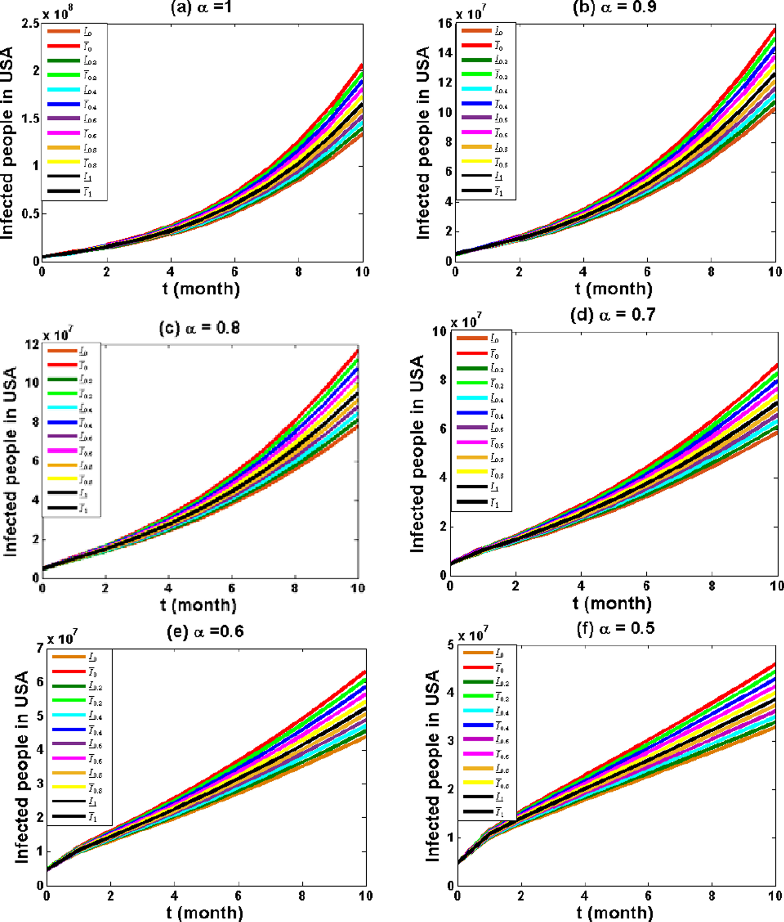
Fig. 2
Numerical results of the number of Exposed cases E (t) in USA for some values of fractional order and distinct values of r = 0, 0.2, 0.4, 0.6, 0.8, 1.0 from August 1, 2020, to May 31, 2021.
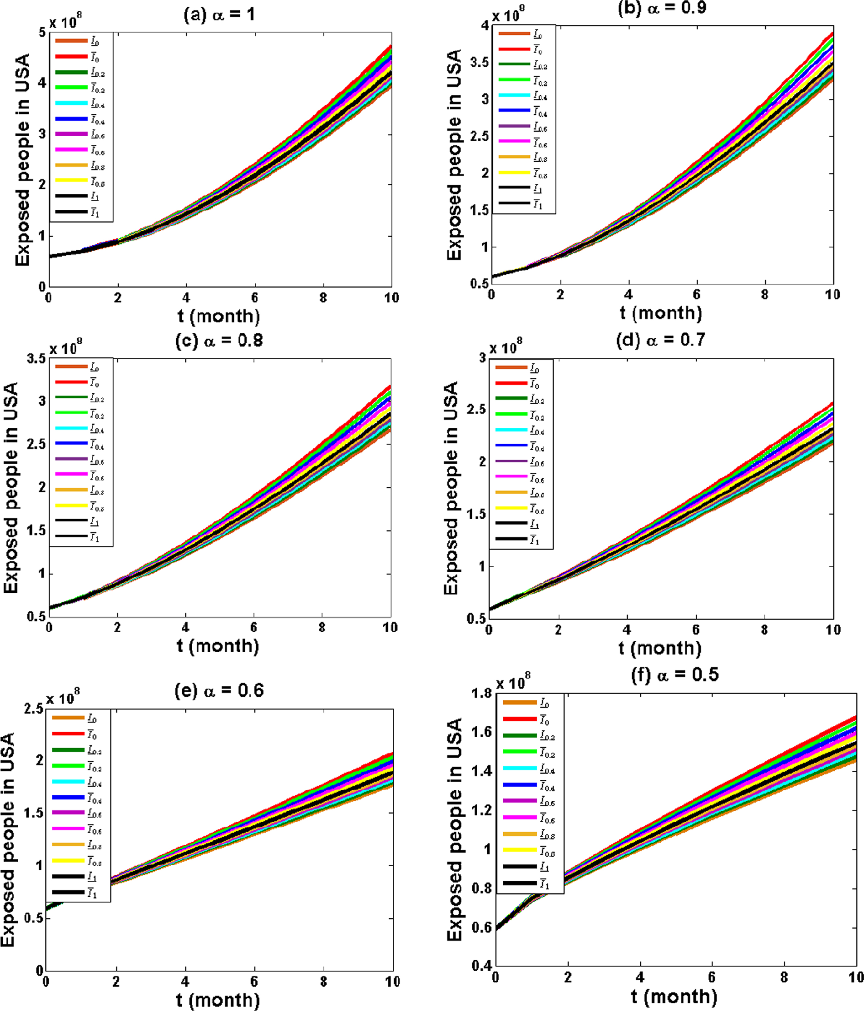
Fig. 3
Numerical results of the number of Susceptible cases S (t) in USA for some values of fractional order and distinct values of r = 0, 0.2, 0.4, 0.6, 0.8, 1.0 from August 1, 2020, to May 31, 2021.
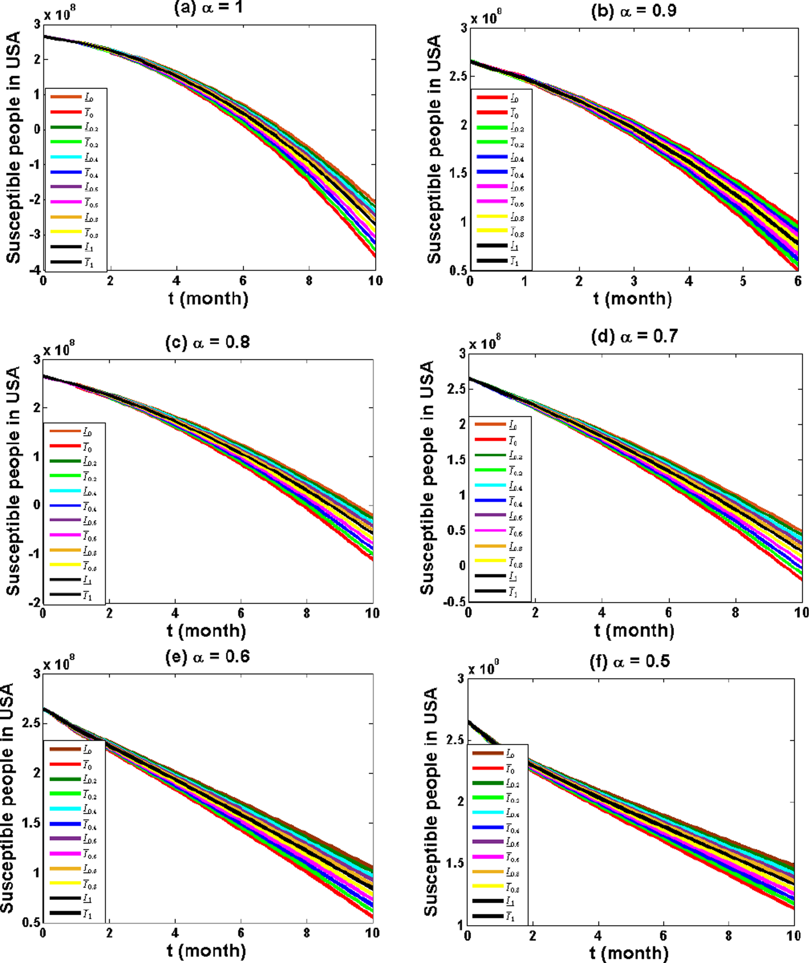
Fig. 4
Numerical results of the number of Recovered cases R (t) in USA for some values of fractional order and distinct values of r = 0, 0.2, 0.4, 0.6, 0.8, 1.0 from August 1, 2020, to May 31, 2021.
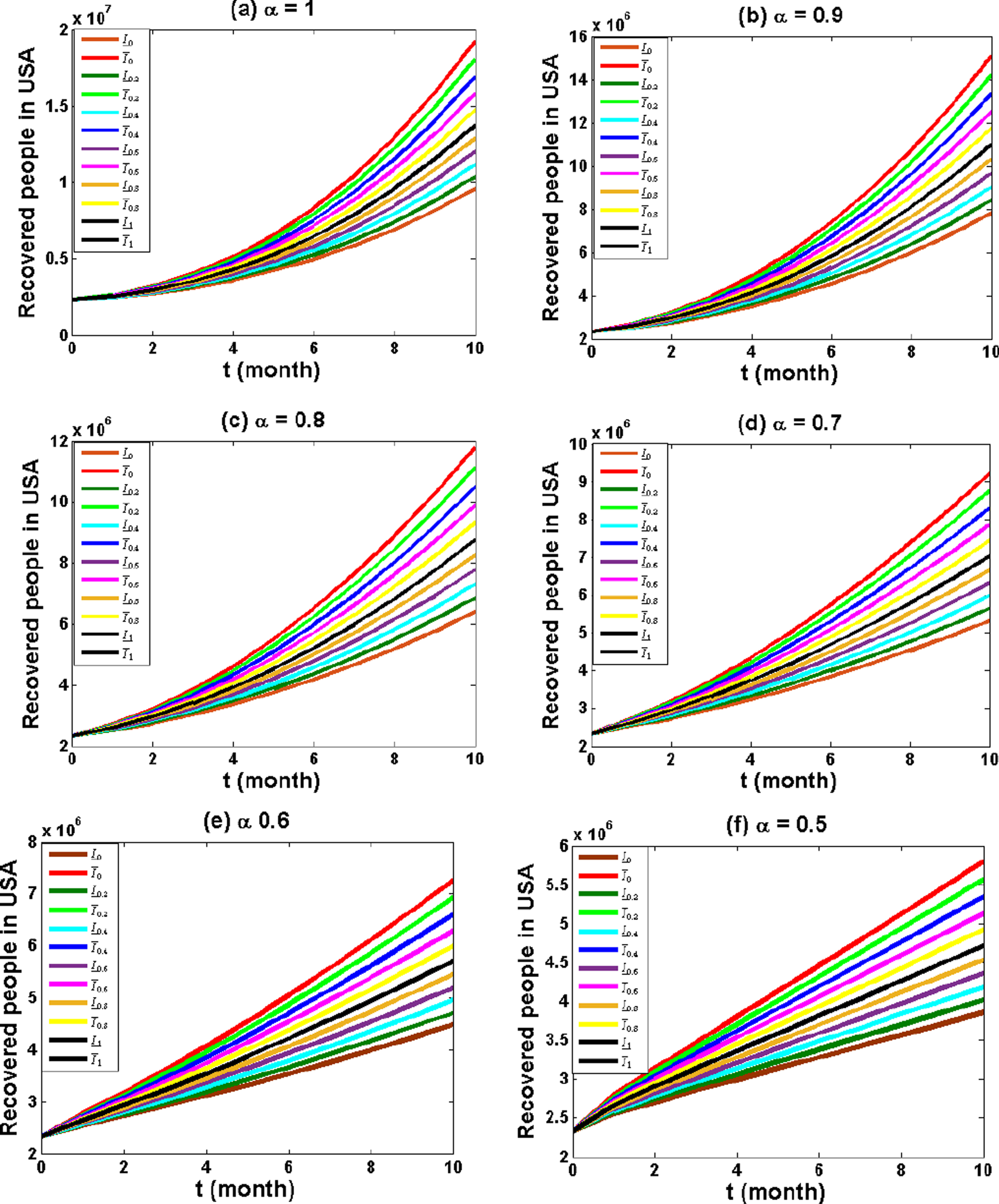
Fig. 5
Numerical results of the number of Infected cases I (t) in INDIA for some values of fractional order and distinct values of r = 0, 0.2, 0.4, 0.6, 0.8, 1.0 from August 1, 2020, to May 31, 2021.
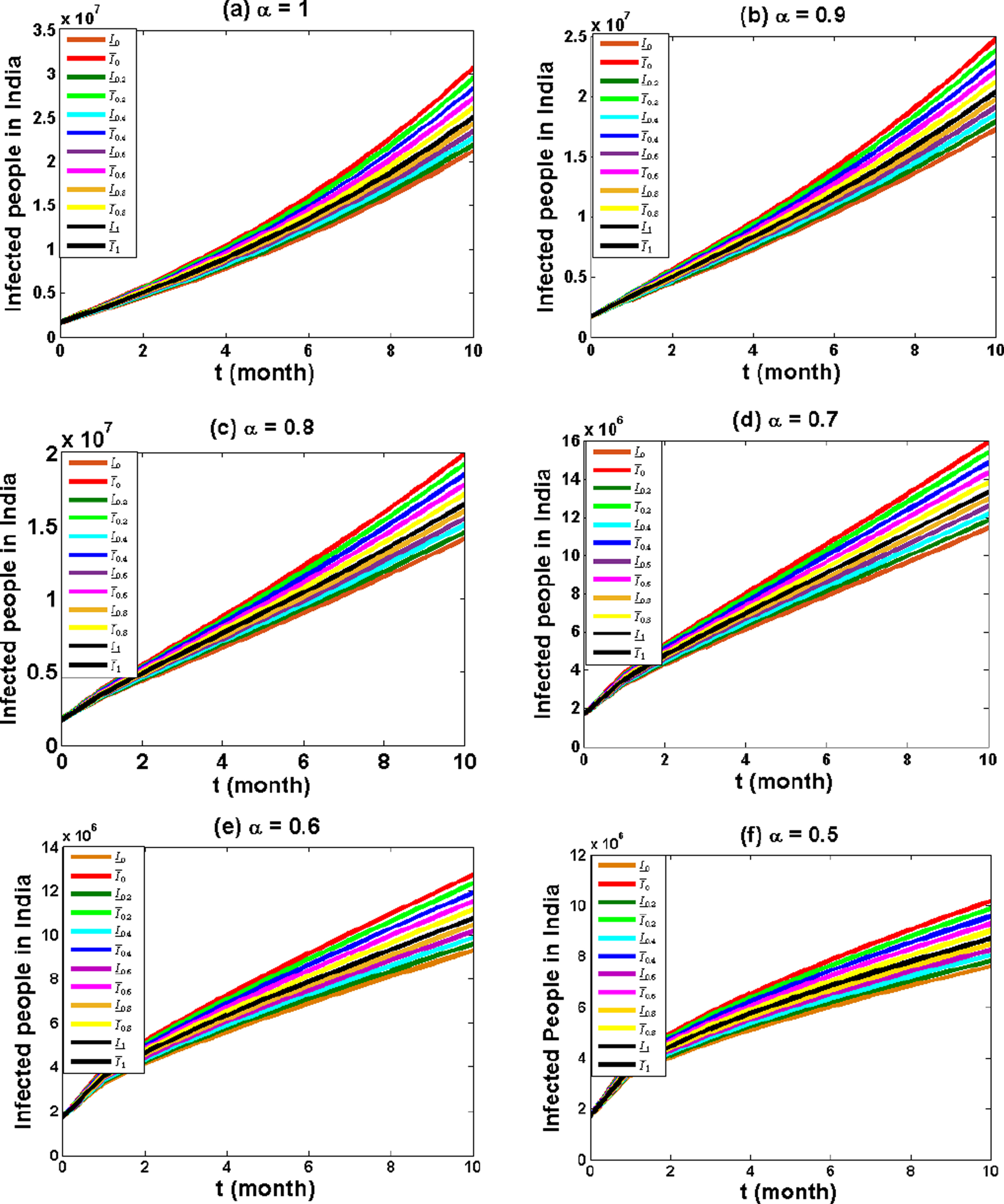
Fig. 6
Numerical results of the number of Exposed cases E (t) in INDIA for some values of fractional order and distinct values of r = 0, 0.2, 0.4, 0.6, 0.8, 1.0 from August 1, 2020, to May 31, 2021.
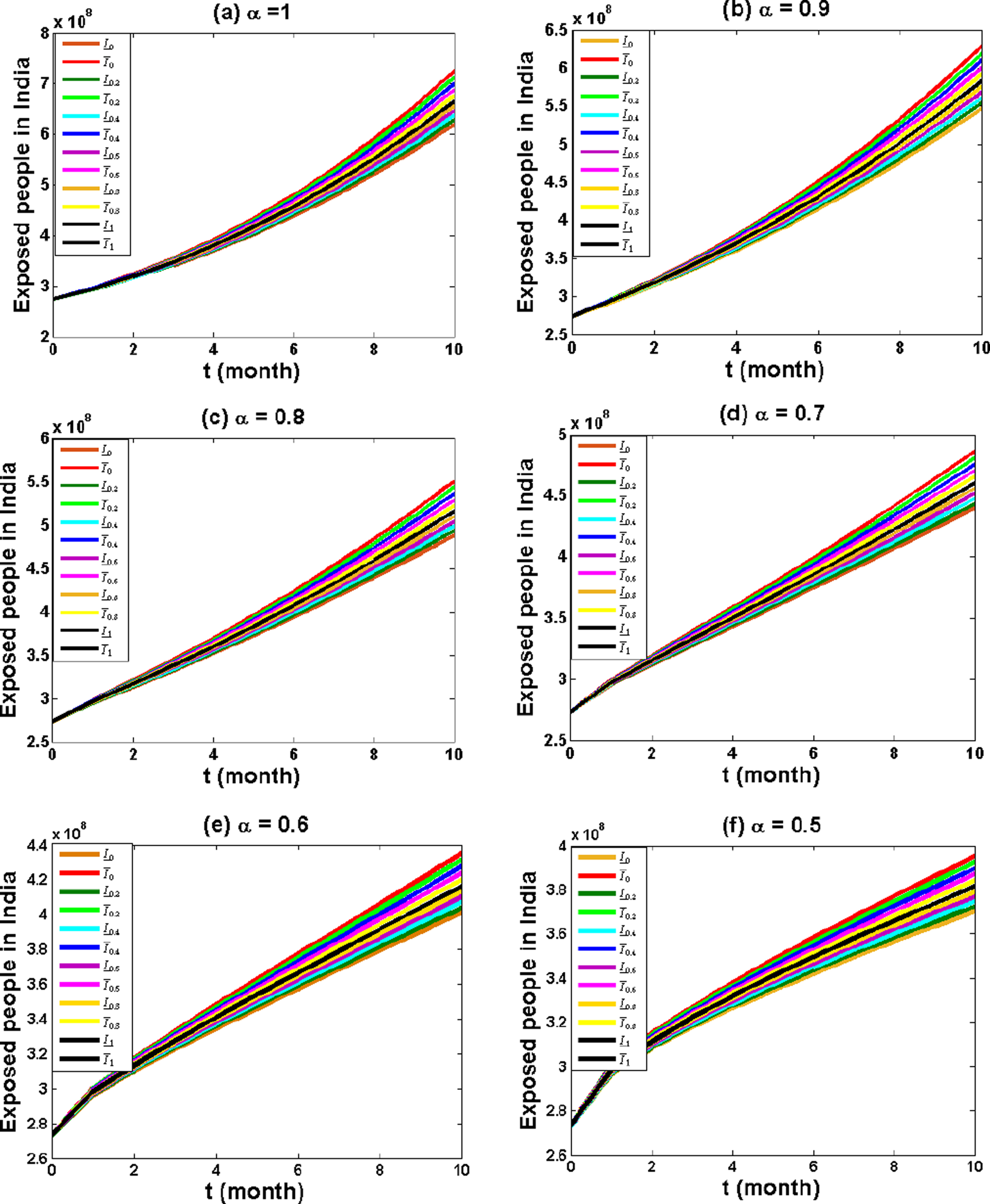
Fig. 7
Numerical results of the number of Susceptible cases S (t) in INDIA for some values of fractional order and distinct values of r = 0, 0.2, 0.4, 0.6, 0.8, 1.0 from August 1, 2020, to May 31, 2021.
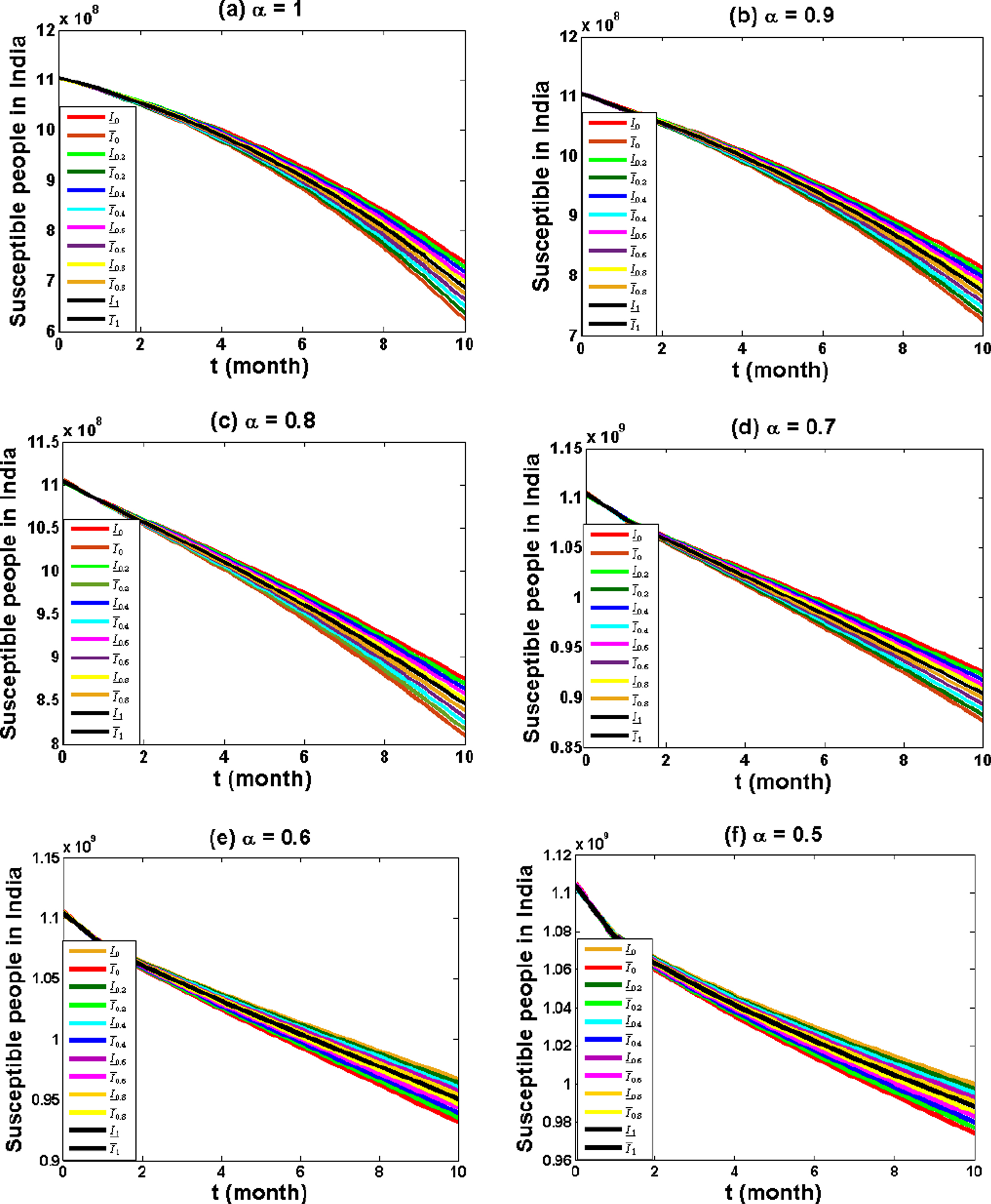
Fig. 8
Numerical results of the number of Recovered cases R (t) in INDIA for some values of fractional order and distinct values of r = 0, 0.2, 0.4, 0.6, 0.8, 1.0 from August 1, 2020, to May 31, 2021.
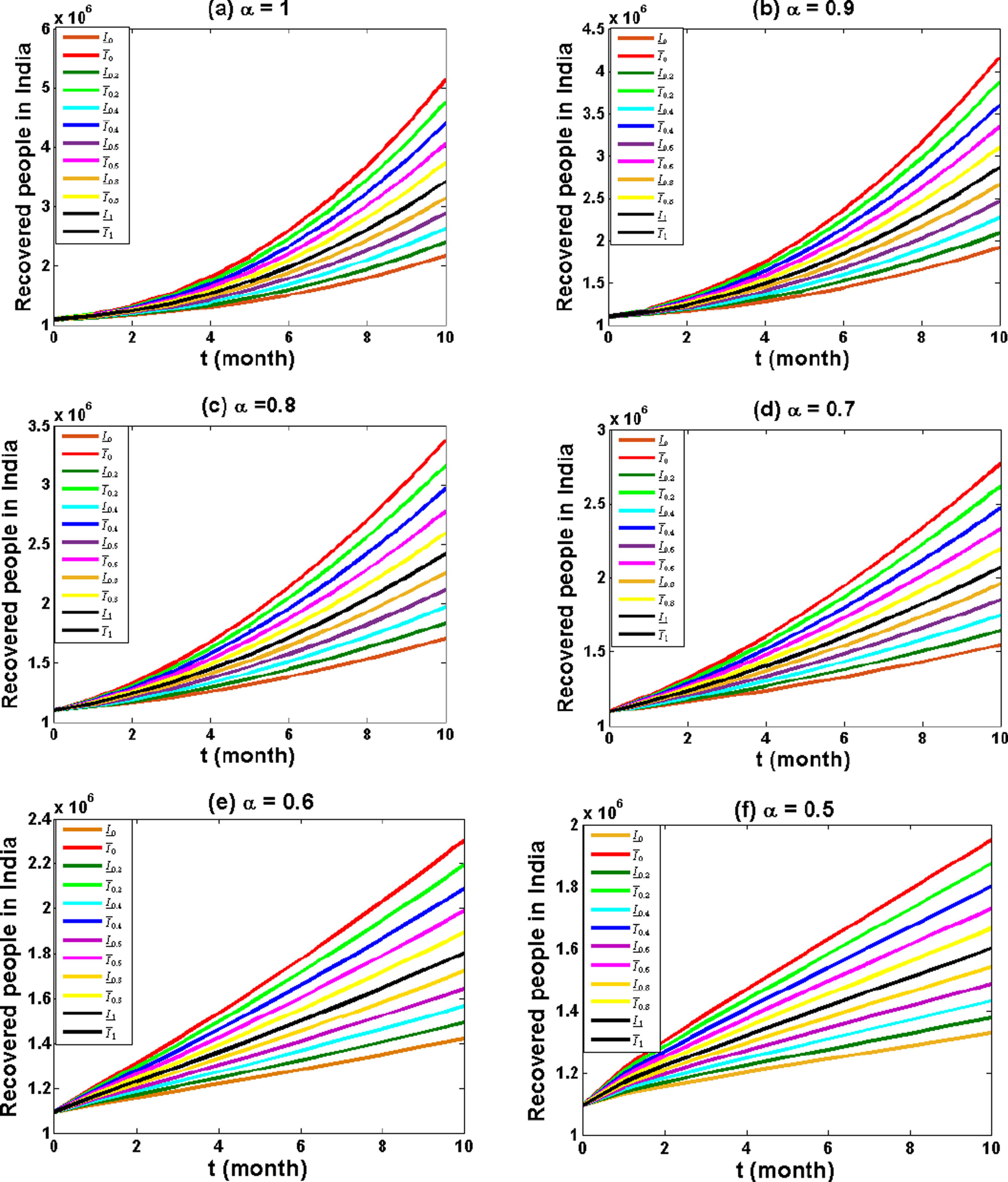
Fig. 9
Numerical results of the number of Infected cases I (t) in ITALY for some values of fractional order and distinct values of r = 0, 0.2, 0.4, 0.6, 0.8, 1.0 from August 1, 2020, to May 31, 2021.
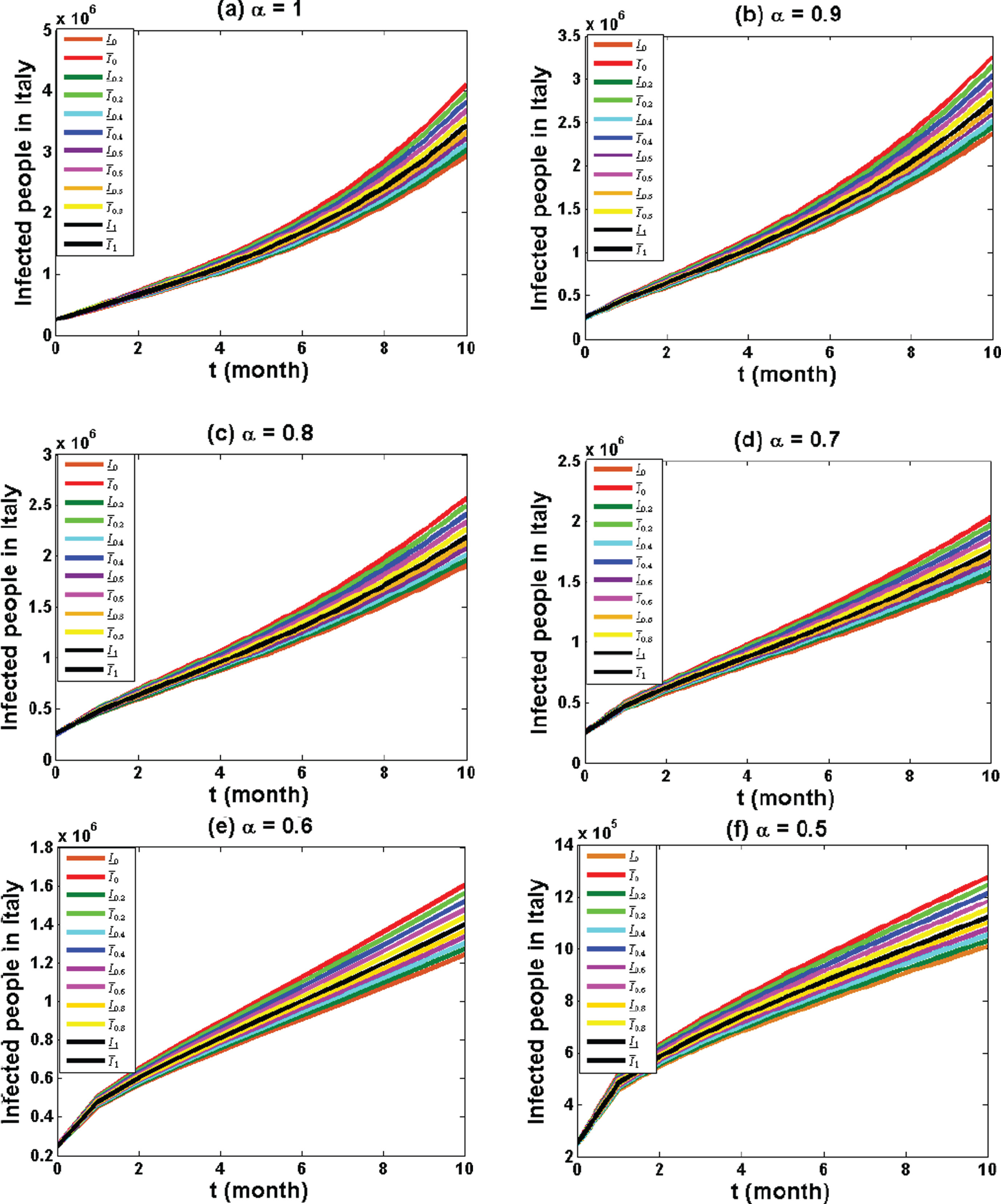
Fig. 10
Numerical results of the number of Exposed cases E (t) in ITALY for some values of fractional order and distinct values of r = 0, 0.2, 0.4, 0.6, 0.8, 1.0 from August 1, 2020, to May 31, 2021.
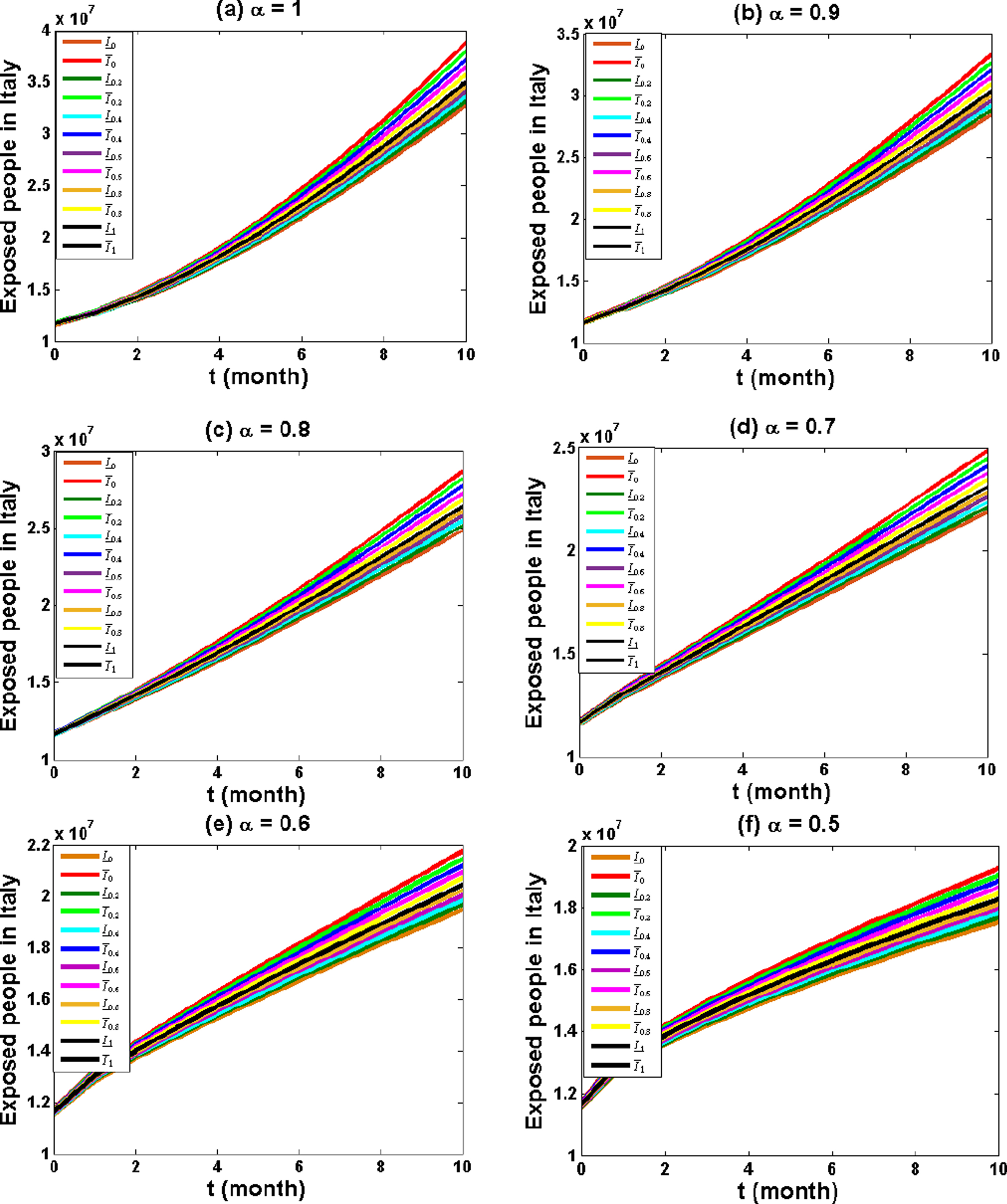
Fig. 11
Numerical results of the number of Susceptible cases S (t) in ITALY for some values of fractional order and distinct values of r = 0, 0.2, 0.4, 0.6, 0.8, 1.0 from August 1, 2020, to May 31, 2021.
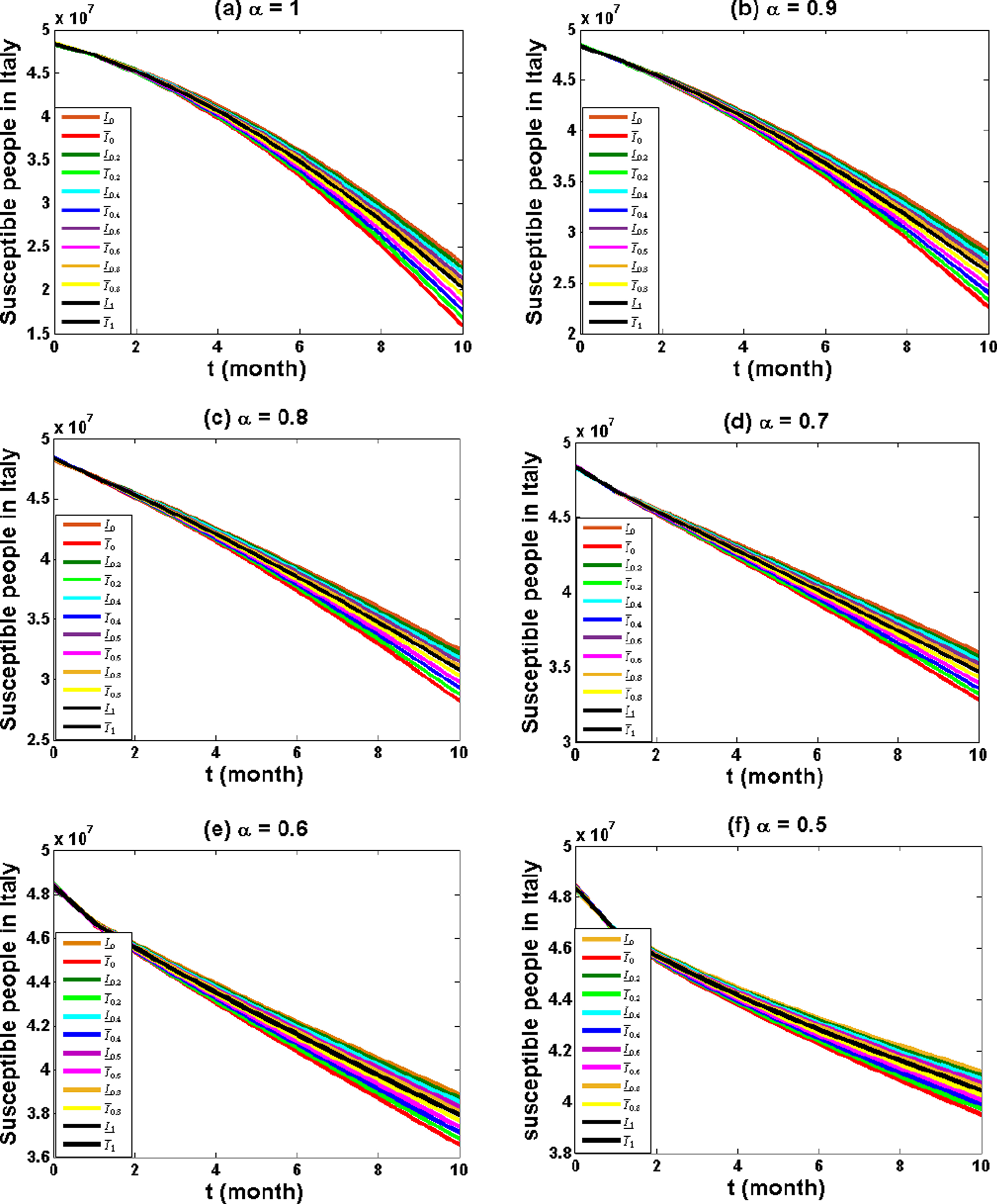
Fig. 12
Numerical results of the number of Recovered cases R (t) in ITALY for some values of fractional order and distinct values of r = 0, 0.2, 0.4, 0.6, 0.8, 1.0 from August 1, 2020, to May 31, 2021.
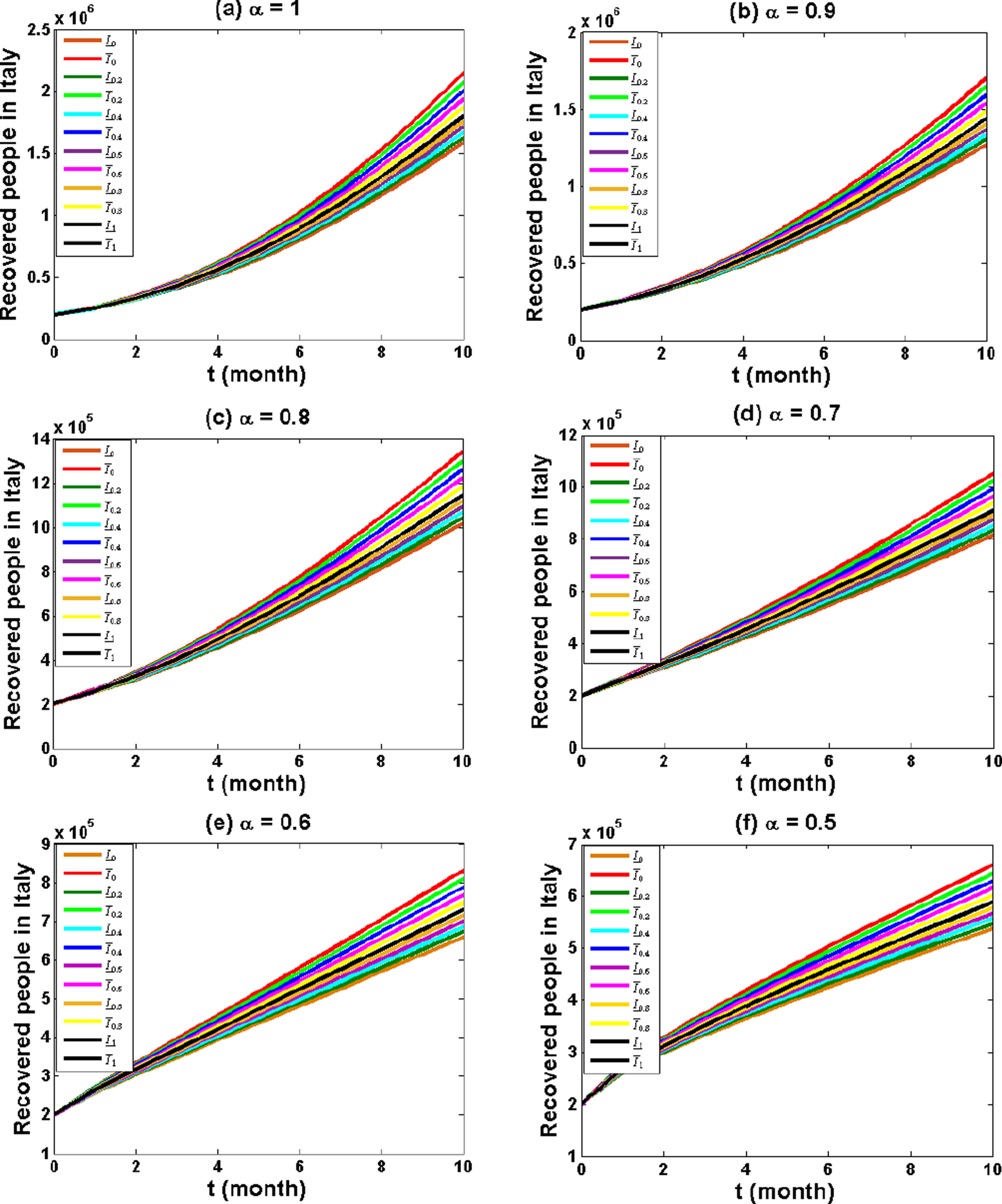
Table 3
Predicted cumulative number of Infected cases I (t) in USA until January 31, 2021
| t = 6 | α = 0.7 | α = 0.8 | α = 0.9 | α = 1 | ||||
|
|
|
|
|
|
|
|
| |
| r = 0 | 3.2220 | 4.4239 | 3.7896 | 5.2634 | 4.4136 | 6.1839 | 5.0868 | 7.1725 |
| r = 0.2 | 3.3236 | 4.2833 | 3.9136 | 5.0904 | 4.5621 | 5.9756 | 5.2614 | 6.9265 |
| r = 0.4 | 3.4271 | 4.1456 | 4.0402 | 4.9211 | 4.7137 | 5.7718 | 5.4396 | 6.6860 |
| r = 0.6 | 3.5327 | 4.0108 | 4.1693 | 4.7556 | 4.8684 | 5.5726 | 5.6214 | 6.4509 |
| r = 0.8 | 3.6403 | 3.8790 | 4.3010 | 4.5937 | 5.0264 | 5.3778 | 5.8071 | 6.2212 |
| r = 1 | 3.7501 | 3.7501 | 4.4354 | 4.4354 | 5.1875 | 5.1875 | 5.9967 | 5.9967 |
Table 4
Predicted cumulative number of Infected cases I (t) in USA until March 31, 2021
| t = 8 | α = 0.7 | α = 0.8 | α = 0.9 | α = 1 | ||||
|
|
|
|
|
|
|
|
| |
| r = 0 | 4.4379 | 6.3340 | 5.5649 | 8.0705 | 6.9136 | 10.156 | 8.4970 | 12.609 |
| r = 0.2 | 4.5964 | 6.1104 | 5.7734 | 7.7741 | 7.1824 | 9.7720 | 8.8370 | 12.121 |
| r = 0.4 | 4.7585 | 5.8921 | 5.9870 | 7.4849 | 7.4581 | 9.3970 | 9.1860 | 11.644 |
| r = 0.6 | 4.9245 | 5.6790 | 6.2058 | 7.2029 | 7.7408 | 9.0310 | 9.5440 | 11.180 |
| r = 0.8 | 5.0943 | 5.4710 | 6.4300 | 6.9278 | 8.0307 | 8.6750 | 9.9110 | 10.728 |
| r = 1 | 5.2681 | 5.2681 | 6.6597 | 6.6597 | 8.3279 | 8.3280 | 10.288 | 10.288 |
Table 5
Predicted cumulative number of Infected cases I (t) in USA until May 31, 2021
| t = 10 | α = 0.7 | α = 0.8 | α = 0.9 | α = 1 | ||||
|
|
|
|
|
|
|
|
| |
| r = 0 | 5.8635 | 8.6235 | 7.7922 | 11.678 | 10.269 | 15.628 | 13.391 | 20.633 |
| r = 0.2 | 6.0927 | 8.2968 | 8.1136 | 11.217 | 10.711 | 14.991 | 13.987 | 19.771 |
| r = 0.4 | 6.3280 | 7.9783 | 8.4440 | 10.768 | 11.166 | 14.371 | 14.600 | 18.932 |
| r = 0.6 | 6.5694 | 7.6680 | 8.7834 | 10.330 | 11.634 | 13.767 | 15.232 | 18.116 |
| r = 0.8 | 6.8171 | 7.3656 | 9.1322 | 9.9050 | 12.115 | 13.180 | 15.883 | 17.323 |
| r = 1 | 7.0712 | 7.0712 | 9.4906 | 9.4910 | 12.610 | 12.610 | 16.552 | 16.552 |
Table 6
Predicted cumulative number of Infected cases I (t) in INDIA until January 31, 2021
| t = 6 | α = 0.7 | α = 0.8 | α = 0.9 | α = 1 | ||||
|
|
|
|
|
|
|
|
| |
| r = 0 | 0.79048 | 1.0591 | 0.9024 | 1.2216 | 1.0264 | 1.4018 | 1.1625 | 1.5993 |
| r = 0.2 | 0.81378 | 1.0279 | 0.9299 | 1.1844 | 1.0586 | 1.3578 | 1.1997 | 1.5478 |
| r = 0.4 | 0.83709 | 0.9972 | 0.9574 | 1.1476 | 1.0907 | 1.3143 | 1.2369 | 1.4970 |
| r = 0.6 | 0.86042 | 0.9668 | 0.9849 | 1.1113 | 1.1229 | 1.2714 | 1.2742 | 1.4470 |
| r = 0.8 | 0.88376 | 0.9368 | 1.0125 | 1.0755 | 1.1551 | 1.2291 | 1.3114 | 1.3975 |
| r = 1 | 0.90713 | 0.9071 | 1.0401 | 1.0401 | 1.1873 | 1.1873 | 1.3488 | 1.3488 |
Table 7
Predicted cumulative number of Infected cases I (t) in INDIA March 31, 2021
| t = 8 | α = 0.7 | α = 0.8 | α = 0.9 | α = 1 | ||||
|
|
|
|
|
|
|
|
| |
| r = 0 | 0.9656 | 1.3213 | 1.1472 | 1.5901 | 1.3594 | 1.9051 | 1.6050 | 2.2705 |
| r = 0.2 | 0.9958 | 1.2793 | 1.1843 | 1.5373 | 1.4046 | 1.8395 | 1.6596 | 2.1899 |
| r = 0.4 | 1.0259 | 1.2379 | 1.2215 | 1.4852 | 1.4500 | 1.7749 | 1.7145 | 2.1106 |
| r = 0.6 | 1.0562 | 1.1970 | 1.2587 | 1.4339 | 1.4955 | 1.7113 | 1.7695 | 2.0325 |
| r = 0.8 | 1.0865 | 1.1567 | 1.2961 | 1.3834 | 1.5412 | 1.6486 | 1.8247 | 1.9557 |
| r = 1 | 1.1169 | 1.1169 | 1.3336 | 1.3336 | 1.5870 | 1.5870 | 1.8802 | 1.8802 |
Table 8
Predicted cumulative number of Infected cases I (t) in INDIA until May 31, 2021
| t = 10 | α = 0.7 | α = 0.8 | α = 0.9 | α = 1 | ||||
|
|
|
|
|
|
|
|
| |
| r = 0 | 1.1433 | 1.5917 | 1.4072 | 1.9890 | 1.7301 | 2.4781 | 2.1215 | 3.0738 |
| r = 0.2 | 1.1806 | 1.5379 | 1.4549 | 1.9185 | 1.7907 | 2.3866 | 2.1976 | 2.9563 |
| r = 0.4 | 1.2180 | 1.4850 | 1.5028 | 1.8492 | 1.8515 | 2.2967 | 2.2742 | 2.8409 |
| r = 0.6 | 1.2555 | 1.4329 | 1.5509 | 1.7809 | 1.9126 | 2.2082 | 2.3513 | 2.7275 |
| r = 0.8 | 1.2932 | 1.3816 | 1.5992 | 1.7138 | 1.9741 | 2.1213 | 2.4289 | 2.6162 |
| r = 1 | 1.3310 | 1.3310 | 1.6478 | 1.6478 | 2.0360 | 2.0360 | 2.5070 | 2.5070 |
Table 9
Predicted cumulative number of Infected cases I (t) in ITALY until January 31, 2021
| t = 6 | α = 0.7 | α = 0.8 | α = 0.9 | α = 1 | ||||
|
|
|
|
|
|
|
|
| |
| r = 0 | 1.0340 | 1.2949 | 1.1730 | 1.4852 | 1.3255 | 1.6939 | 1.4908 | 1.9196 |
| r = 0.2 | 1.0555 | 1.2638 | 1.1986 | 1.4479 | 1.3555 | 1.6496 | 1.5255 | 1.8678 |
| r = 0.4 | 1.0774 | 1.2333 | 1.2246 | 1.4111 | 1.3860 | 1.6060 | 1.5607 | 1.8168 |
| r = 0.6 | 1.0995 | 1.2032 | 1.2509 | 1.3750 | 1.4168 | 1.5632 | 1.5964 | 1.7668 |
| r = 0.8 | 1.1219 | 1.1737 | 1.2775 | 1.3395 | 1.4481 | 1.5211 | 1.6326 | 1.7176 |
| r = 1 | 1.1446 | 1.1446 | 1.3046 | 1.3046 | 1.4798 | 1.4798 | 1.6694 | 1.6694 |
Table 10
Predicted cumulative number of Infected cases I (t) in ITALY until March 31, 2021
| t = 8 | α = 0.7 | α = 0.8 | α = 0.9 | α = 1 | ||||
|
|
|
|
|
|
|
|
| |
| r = 0 | 1.2742 | 1.6429 | 1.5126 | 1.9816 | 1.7912 | 2.3794 | 2.1123 | 2.8399 |
| r = 0.2 | 1.3044 | 1.5988 | 1.5507 | 1.9252 | 1.8387 | 2.3084 | 2.1707 | 2.7516 |
| r = 0.4 | 1.3351 | 1.5554 | 1.5895 | 1.8698 | 1.8871 | 2.2387 | 2.2302 | 2.6651 |
| r = 0.6 | 1.3662 | 1.5129 | 1.6290 | 1.8155 | 1.9364 | 2.1704 | 2.2909 | 2.5804 |
| r = 0.8 | 1.3979 | 1.4711 | 1.6691 | 1.7622 | 1.9866 | 2.1034 | 2.3528 | 2.4973 |
| r = 1 | 1.4301 | 1.4301 | 1.7100 | 1.7100 | 2.0377 | 2.0377 | 2.4160 | 2.4160 |
Table 11
Predicted cumulative number of Infected cases I(t) in ITALY until May 31, 2021
| t = 10 | α = 0.7 | α = 0.8 | α = 0.9 | α = 1 | ||||
|
|
|
|
|
|
|
|
| |
| r = 0 | 1.5359 | 2.0309 | 1.9068 | 2.5727 | 2.3676 | 3.2522 | 2.9327 | 4.0920 |
| r = 0.2 | 1.5763 | 1.9716 | 1.9608 | 2.4927 | 2.4392 | 3.1458 | 3.0263 | 3.9525 |
| r = 0.4 | 1.6174 | 1.9135 | 2.0161 | 2.4144 | 2.5125 | 3.0417 | 3.1222 | 3.8159 |
| r = 0.6 | 1.6594 | 1.8565 | 2.0725 | 2.3377 | 2.5874 | 2.9398 | 3.2203 | 3.6823 |
| r = 0.8 | 1.7022 | 1.8006 | 2.1301 | 2.2625 | 2.6640 | 2.8400 | 3.3209 | 3.5516 |
| r = 1 | 1.7458 | 1.7458 | 2.1889 | 2.1889 | 2.7423 | 2.7423 | 3.4238 | 3.4238 |
From Tables 6, 7, and 8, we can observe that the number of people infected with COIVD-19 predicted for the end of months January, March, and May for India might be as high as between 0.9024 × 10⁷ and 1.2216 × 10⁷ at α = 0.8, between 0.9656 × 10⁷ and 1.3213 × 10⁷ at α = 0.7 and between 2.1215 × 10⁷ and 3.0738 × 10⁷ at α = 1. From this, the predicted values of infected cases for India obtained by our proposed model are much closed to the actual data. Similarly, we can see that the predicted number of infected cases with COIVD-19 for the end of months January, March, and May for other two countries USA and Italy are extremely close to the actual data. As a result, our proposed model is well-trained and capable of predicting novel coronaviruses in the future.
From the outcomes of figures and tables referenced here, we can express that as the fractional derivative order α decrease, the number of infected people decrease significantly. Moreover, the fuzzy fractional derivative model gives more accurate results than the classical derivative model and permits better examine the obtained results.
4Stability analysis
The equilibrium points are found by setting
This implies, we have
The Jacobian matrix of model (2) can be computed as follows.
The Jacobian matrix at the equilibrium point is given by
The characteristic equation of the matrix J is obtained by
(3)
Where,
On substituting the values of all parameters and solving the characteristic Equation (3), we obtain eigenvalues that are λ1 = λ2 = 0 and the roots of the equation λ2 + Aλ + B = 0.
Since the two roots of the equation λ2 + Aλ + B = 0 are negative, the system is asymptotically stable.
5Comparison of results
In this section, we compare our model with Ahmadian’s fuzzy fractional model of coronavirus in [35] which is based on the fractional model in [23].
(4)
where N represents the whole variety of people, N is isolated into five-compartment: Susceptible cases (S), Exposed cases (E), Infected cases (I), Asymptotically infected cases (A) and Eliminated or Recovered cases (R). The human beings in the store or market are represented by Q. For r ∈ [0, 1]
Here, we analyze model (4) for India. For this, we reflect on consideration on all parametric values from the literature [23] where the following data are considered from March 14, 2020, till March 26, 2020.
The whole population of India N = 1, 352, 600, 000, E (0) = 1, 724, 266, I (0) = 745, A (0) = 413, R (0) = 66, S (0) = 1, 350, 900, 000 and Q (0) = 10, 000. The parameter values are Δ = 53, 320.19,
6Numerical results and discussion
In Fig. 13(a) and 13(b), we have plotted numerical results of infected cases of Ahmadian’s model (4) for India at α = 1 and α = 0.9 with different values of r. Table 12 shows the comparison between the numerical solution of infected cases of COVID-19 for our proposed model (2) and Ahmadian’s model (4).
Fig. 13
Numerical results of the number of Infected people I (t) in INDIA for some values of fractional order and distinct values of r = 0, 0.2, 0.4, 0.6, 0.8, 1.0 up to mid-Nov 2020.
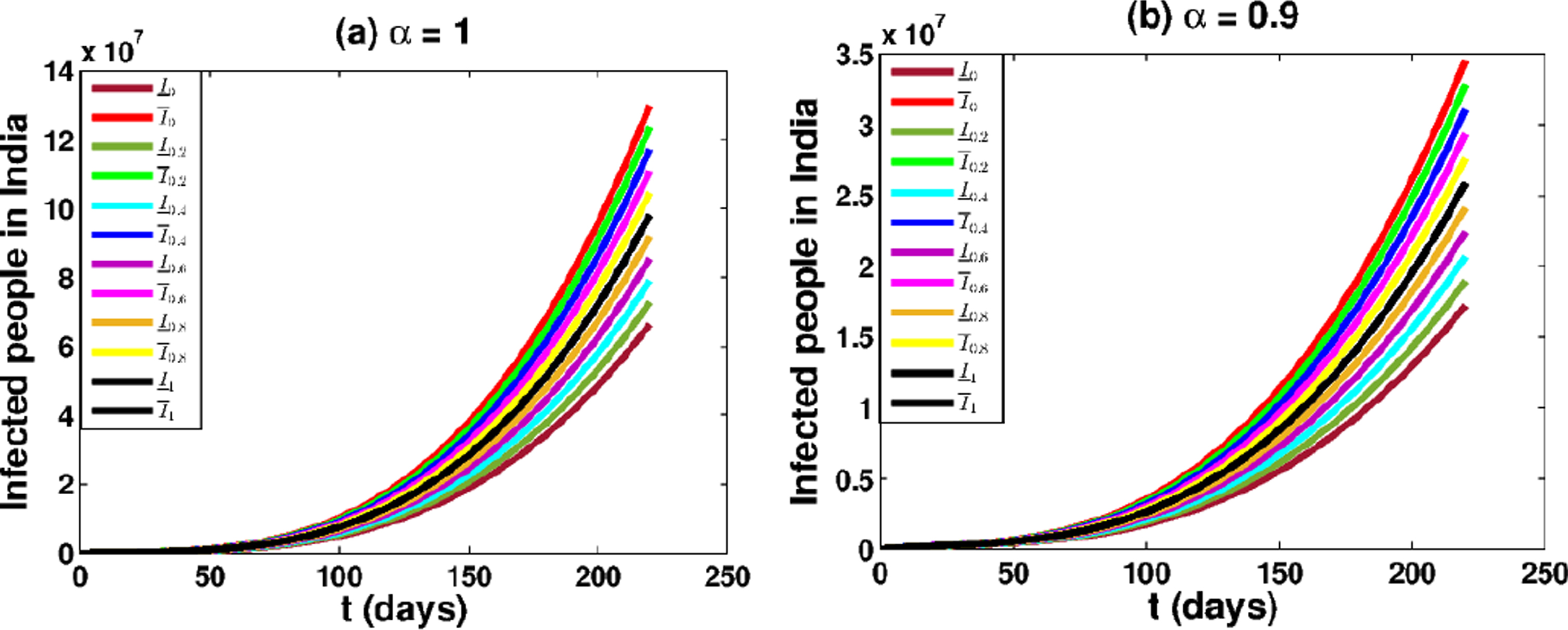
Table 12
Comparison between the numerical solution of infected people of the proposed model and Ahmadian’s model for India
| t (month) | Our proposed model (r = 0) | t (days) | Ahmadian’s model (r = 0) | ||
|
α = 1
|
α = 0.9
|
α = 1
|
α = 0.9
| ||
| 1 | [3.0833 × 10⁶, 3.6234 × 10⁶] | [3.1451 × 10⁶, 3.7110 × 10⁶] | 150 | [1.8801 × 10⁷, 3.7915 × 10⁷] | [5.5340 × 10⁶, 1.1314 × 10⁷] |
| 2 | [4.5589 × 10⁶, 5.6972 × 10⁶] | [4.4873 × 10⁶, 5.6012 × 10⁶] | 180 | [3.4366 × 10⁷, 6.8303 × 10⁷] | [9.4863 × 10⁶, 1.9250 × 10⁷] |
| 3 | [6.1371 × 10⁶, 7.9449 × 10⁶] | [5.8485 × 10⁶, 7.5439 × 10⁶] | 210 | [5.6988 × 10⁷, 1.1194 × 10⁸] | [1.4997 × 10⁷, 3.0157 × 10⁷] |
| 4 | [7.8317 × 10⁶, 1.0393 × 10⁷] | [7.2557 × 10⁶, 9.5793 × 10⁶] | 240 | [8.8004 × 10⁷, 1.7126 × 10⁸] | [2.2288 × 10⁷, 4.4432 × 10⁷] |
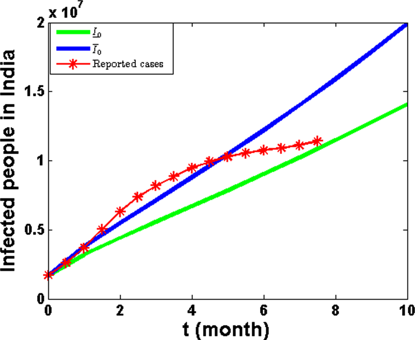
The reported cases and fitted curve of the proposed model for COVID-19 in India from August 2020 to May 2021 for α = 0.8 at r = 0 are plotted in Fig. 14. Figure 14 shows that the numerical results of the proposed model (2) correspond well with the real data for α = 0.8. In Table 12, the proposed model gives that the prediction of cumulative infected cases in India at the end of November may reach between 7.2557 × 10⁶ and 9.5793 × 10⁶ for α = 0.9 and also 7.8317 × 10⁶ and 1.0393 × 10⁷ for α = 1. But Ahmadian’s model gives that the prediction of cumulative infected cases in India at the end of November may reach between 2.2288 × 10⁷and 4.4432 × 10⁷ for α = 0.9 and also 8.8004 × 10⁷ and 1.7126 × 10⁸ for α = 1. So, we can see that our proposed model offers better prediction effects of infected cases than Ahmadian’s model. The main advantage of our proposed model is that our mathematical model contains fewer parameters compare to Ahmadian’s model. So, we have less computation work. Also, our model gives a superior fit to the actual data. We truly hope that our model could help the decision-making of epidemic prevention and control strategy for governments of different countries in COVID-19. The Government of India has forced 21 days cross country lockdown from 25 March 2020 and asymptomatic and symptomatic cases are quickly position in isolation. The impact of these prevention measures suggests that the spread of the virus can be decreased significantly.
Fig. 14
The Reported cases from August 1, 2020, to March 15, 2021, and the fitted curve of the proposed model for COVID-19 in India from August 1, 2020, to May 31, 2021, dashed-dotted line represents Reported cases and solid line represents fitted curve.
7Limitations
This model used to be designed to see transmission dynamics so does not to depict infection seriousness and demise. Without external births and deaths, the population’s size is assumed to be stable. This assumption is likely to have a significant impact given the time frame for investigating epidemics here. Further, this model does not separate the asymptomatic from pre-symptomatic. To overcome these limitations, we can extend the proposed model with more compartments such as symptomatic, asymptomatic, and quarantined cases to describe the dynamics of the COVID-19 epidemic process.
8Conclusion
In this paper, we studied the mathematical model of Caputo fractional derivative under fuzzy sense for the prediction of COVID-19. The data up to July 31, 2020, was utilized for finding parameters of the model with the best fit. Firstly, numerical simulations have been performed to predict COVID-19 cases in USA, India, and Italy over 10 months. Moreover, we have presented the results of the fractional-order model with the results of the integer-order model. The graphical representations are exhibited for the different values of α using MATLAB. The results confirmed that the fuzzy fractional-order model gives a superior fit to the real information with considerably less error than the integer-order model. Secondly, stability analysis has been provided for the proposed model in fuzzy environment. Lastly, the results of our suggested model have been compared with Ahmadian’s fuzzy fractional model. It is proven that the number of infected humans will increase with an increment in contact rate. Therefore, if we need to end this outbreak pandemic we have to be quarantined to decrease the conduct rate. In future studies, we can combine more compartments such as symptomatic, asymptomatic, and quarantined cases into our present model so that the model can give better depict the spread of infectious diseases and forecast the future trends and also investigate the applicability of the present model in various epidemic viruses.
References
[1] | Wang C. , Horby P.W. , Hayden F.G. and Gao G.F. , A novel coronavirus outbreak of global health concern, The Lancet 395: (10233) ((2020) ), 470–473. |
[2] | Gorbalenya A.E. , Baker S.C. , Baric R. , Groot R.J.D. , Drosten C. , Gulyaeva A.A. ,... and Ziebuhr J. , Severe acute respiratory syndrome-related coronavirus: The species and its viruses a statement of the Coronavirus Study Group (2020). |
[3] | Organization WH. Naming the coronavirus disease (COVID-19) and the virus that causes it. https://www.who.int/emergencies/diseases/novel-coronavirus-019/technical-guidance/naming-the-coronavirus-disease-(covid-2019)-andthe-virus-that-causes-it; (2020) a. |
[4] | Elmousalami H.H. and Hassanien A.E. , Day level forecasting for Coronavirus Disease (COVID- 19) spread: analysis, modeling and recommendations, arXiv preprint arXiv:2003.07778 (2020). |
[5] | Bassetti M. , Vena A. and Giacobbe D.R. , The novel chinese coronavirus -nCoV) infections: challenges for fighting the storm, European Journal of Clinical Investigation 50: (3) ((2020) ). |
[6] | Rothan H.A. and Byrareddy S.N. , The epidemiology and pathogenesis of coronavirus disease (COVID-19) outbreak, Journal of Autoimmunity 109: ((2020) ), 102433. |
[7] | World Health Organization, Coronavirus disease 2019 (COVID-19) Situation Report-193. |
[8] | Bai Y. , Yao L. , Wei T. , Tian F. , Jin D.Y. , Chen L. and Wang M. , Presumed asymptomatic carrier transmission of COVID-19, Jama 323: (14) ((2020) ), 1406–1407. |
[9] | Egonmwan A.O. and Okuonghae D. , Mathematical analysis of a tuberculosis model with imperfect vaccine, International Journal of Biomathematics 12: (07) ((2019) ), 1950073. |
[10] | Nwankwo A. and Okuonghae D. , A mathematical model for the population dynamics of malaria with a temperature dependent control, Differential Equations and Dynamical Systems (2019), 1–30. |
[11] | Okuonghae D. , Backward bifurcation of an epidemiological model with saturated incidence, isolation and treatment functions, Qualitative Theory of Dynamical Systems 18: (2) ((2019) ), 413–440. |
[12] | Aslan I.H. , Demir M. , Wise M.M. and Lenhart S. , Modeling COVID-19: Forecasting and analyzing the dynamics of the outbreak in Hubei and Turkey. MedRxiv preprint (2020). |
[13] | Atangana A. , Modelling the spread of COVID-19 with new fractal-fractional operators: can the lockdown save mankind before vaccination? Chaos, Solitons & Fractals 136: ((2020) ), 109860. |
[14] | Hellewell J. , Abbott S. , Gimma A. , Bosse N.I. , Jarvis C.I. , Russell T.W. ,... and Eggo R.M. , Feasibility of controlling COVID-19 outbreaks by isolation of cases and contacts, The Lancet Global Health 8: (4) ((2020) ), e488–e496. |
[15] | Ivorra B. , Ferrandez M.R. , Vela-Pérez M. and Ramos A.M. , Mathematical modeling of the spread of the coronavirus disease (COVID-19) taking into account the undetected infections. The caseof China, Communications in Nonlinear Science NumericalSimulation 88: ((2020) ), 105303. |
[16] | Kucharski A.J. , Russell T.W. , Diamond C. , Liu Y. , Edmunds J. , Funk S. ,... and Flasche S. , Early dynamics of transmission and control of COVID-19: a mathematical modelling study, The Lancet Infectious Diseases 20: (5) ((2020) ), 553–558. |
[17] | Shim E. , Tariq A. , Choi W. , Lee Y. and Chowell G. , Transmission potential and severity of COVID-19 in South Korea, International Journal of Infectious Diseases 93: ((2020) ), 339–344. |
[18] | Okuonghae D. and Omame A. , Analysis of a mathematical model for COVID-19 population dynamics in Lagos, Nigeria, Chaos, Solitons & Fractals 139: ((2020) ), 110032. |
[19] | Podlubny I. , Fractional differential equations: an introduction to fractional derivatives, fractional differential equations, to methods of their solution and some of their applications, Elsevier ((1998) ). |
[20] | Samko S.G. , Kilbas A.A. and Marichey O.I. , Fractional integrals and derivatives, theory and applications, Gordon and Breach, Yverdon. (1993a). |
[21] | González-Parra G. , Arenas A.J. and Chen-Charpentier B.M. , Afractional order epidemic model for the simulation of outbreaks ofinfluenza A (H1N1), Mathematical methods in the AppliedScience 37: (15) ((2014) ), 2218–2226. |
[22] | Khan M.A. and Atangana A. , Modeling the dynamics of novel coronavirus (2019-nCov) with fractional derivative, Alexandria Engineering Journal 59: (4) ((2020) ), 2379–2389. |
[23] | Shaikh A.S. , Shaikh I.N. and Nisar K.S. , A mathematical model of covid-19 using fractional derivative: Outbreak in India with dynamics of transmission and control, Advances in Difference Equations 2020: (1) ((2020) ), 1–19. |
[24] | Chen Y. , Cheng J. , Jiang X. and Xu X. , The reconstruction and prediction algorithm of the fractional TDD for the local outbreak of COVID-19, arXiv preprint arXiv:2002.10302 (2020). |
[25] | Tuan N.H. , Mohammadi H. and Rezapour S. , A mathematical model for COVID-19 transmission by using the Caputo fractional derivative, Chaos, Solitons & Fractals 140: ((2020) ), 110107. |
[26] | Rajagopal K. , Hasanzadeh N. , Parastesh F. , Hamarash I.I. , Jafari S. and Hussain I. , A fractional-order model for the novel coronavirus (COVID-19) outbreak, Nonlinear Dynamics 101: (1) ((2020) ), 711–718. |
[27] | Zadeh L.A. , Fuzzy set, Information and Control 8: (3) ((1965) ), 338–353. |
[28] | Ebrahimnejad A. , New method for solving fuzzy transportation problems with LR flat fuzzy numbers, Information Sciences 357: ((2016) ), 108–124. |
[29] | Ebrahimnejad A. and Verdegay J.L. , Fuzzy sets-based methods and techniques for modern analytics (Vol. 364) Springer ((2018) ). |
[30] | Ebrahimnejad A. , Verdegay J.L. and Garg H. , Signed distance ranking based approach for solving bounded interval-valued fuzzy numbers linear programming problems, International Journal of Intelligent Systems 34: (9) ((2019) ), 2055–2076. |
[31] | Ebrahimnejad A. , An effective computational attempt for solving fully fuzzy linear programming using MOLP problem, Journal of Industrial and Production Engineering 36: (2) ((2019) ), 59–69. |
[32] | Biswas S. and Roy T.K. , A semianalytical method for fuzzy integro-differential equations under generalized seikkala derivative, Soft Computing 23: (17) ((2019) ), 7959–7975. |
[33] | Biswas S. , Moi S. and Sarkar S.P. , Numerical solution of fuzzy Fredholm integro-differential equations by polynomial collocation method, Computational and Applied Mathematics 40: (7) ((2021) ), 1–33. |
[34] | El Allaoui A. , Melliani S. and Chadli L.S. , A Mathematical modeling and epidemic prediction of COVID-19, Available at SSRN 3580162 (2020). |
[35] | Ahmad S. , Ullah A. , Shah K. , Salahshour S. , Ahmadian A. and Ciano T. , Fuzzy fractional-order model of the novel coronavirus, Advances in Difference Equations 2020: (1) ((2020) ), 1–17. |
[36] | Salahshour S. , Allahviranloo T. , Abbasbandy S. and Baleanu D. , Existence and uniqueness results for fractional differential equations with uncertainty, Advances in Difference Equations 2012: (1) ((2012) ), 1–12. |
[37] | De Barros L.C. , Bassanezi R.C. and Lodwick W.A. , First Course in Fuzzy Logic, Fuzzy Dynamical Systems, and Biomathematics, Springer-Verlag Berlin An. ((2016) ). |
[38] | Chalco-Cano Y. and Roman-Flores H. , On new solutions of fuzzy differential equations, Chaos, Solitons & Fractals 38: (1) ((2008) ), 112–119. |
[39] | Allahviranloo T. , Salahshour S. and Abbasbandy S. , Explicit solutions of fractional differential equations with uncertainty, Soft Computing 16: (2) ((2012) ), 297–302. |
[40] | Worldometer: COVID-19 coronavirus pandemic. American Library Association. https://www.worldometers.info/coronavirus. |


