
Automatic segmentation of liver/kidney area with double-layered fuzzy C-means and the utility of hepatorenal index for fatty liver severity classification
Abstract
Background:
Hepatorenal index (HRI) has been an efficient and simple quantified measure in distinction between normal and abnormalities of diagnosing fatty liver. However, considering the clinical significance, the diagnosis of severity stage is more important and single HRI cutoff may not be enough. Also, the segmentation of Liver/Kidney area should be automatic to get rid of operator subjectivity from ultrasonography analysis.
Method:
Double-layered Fuzzy C-Means (DFCM) pixel clustering method is proposed to extract the target area of analysis automatically. HRI and other shape related variables of Liver intensity distribution such as the skewness, the kurtosis, and the coefficient of variance (CV) are automatically computed for the fatty liver severity stage classification.
Result:
From fifty ultrasound images obtained from regular health checkup with 24 normal, 12 mild, 11 moderate, 3 severe stage determined by three different radiologists, the proposed DFCM automatically extracts the region of interests(ROI) and generates a set of statistically significant variables including HRI, the skewness, the kurtosis, the coefficient of variance of liver intensity distribution as well as liver echogenicity. In severity stage classification, the echogenicity of the liver and distribution shape variables such as the skewness and the kurtosis are better predictors than HRI based on our simple decision tree learning analysis.
Conclusion:
For better diagnosis of fatty liver severity stages, we need better set of features than the single HRI cutoff. Better machine learning structures are necessary in this severity stage classification problem with automatic segmentation method proposed in this paper.
1Introduction
The nonalcoholic fatty liver disease (NAFLD) is the most common liver abnormality. NAFLD is now the leading cause of chronic liver disease in the United States and Europe and increasing worldwide. The prevalence of NAFLD in the general population is estimated to be 20–30% in western countries [1, 2], but the number is also rapidly approaching to that ratio in Eastern Asian countries due to the westernization of the diet, aging of society, and reduced physical activity [3, 4]. In mild forms, fatty liver can be a reversible condition that may improve with lifestyle modifications such as diet changes, weight loss, and increased physical activity. However, it is reported that as much as 23% of patients with simple steatosis may still develop nonalcoholic steatohepatitis (NASH) and fibrosis progression, as demonstrated in a recent 3-year follow-up of NAFLD patients [5]. NAFLD is closely associated with central adiposity, type 2 diabetes mellitus, dyslipidemia, and insulin resistance [6] such that NAFLD predicts the tendency to develop both diabetes mellitus [7] and cardiovascular disease [8]. NAFLD is not a rare disease in the non-obese population either. NAFLD was found in 12.6% of non-obese subjects and 50.1% of obese subjects from a routine health evaluation checkup of 29,994 subjects thus it should also be considered a meaningful predictor of metabolic diseases in the non-obese population [4].
The severity of NAFLD was divided into mild (slight increase in liver echogenicity, mild attenuation of the penetration of ultrasound signal, and slight decreased lucidity of the borders of intrahepatic vessels walls and diaphragm), moderate (diffuse increase of liver echogenicity, greater attenuation of the penetration of ultrasound signal, decrease of the visualization of intrahepatic vessels walls, particularly the peripheral branches), and severe (gross increase of liver echogenicity, greater reduction of penetration of ultrasound signal, and poor or no visualization of intrahepatic vessels walls and diaphragm) [9]. It is reported that patients with higher ultrasound grades of liver steatosis are under increased risk of metabolic syndrome independently of age, gender, body mass index (BMI), and impaired glucose metabolism [10].
Liver biopsy is the gold standard for the quantification of hepatic steatosis. However, it is difficult for most patients to accept it due to its invasiveness and a significant degree of sampling error [11]. In view of the public health issue of the increasing prevalence of NAFLD and its hepatic and extrahepatic consequences, the development of simple cost-effective screening methods has become extremely important [12].
Ultrasonography is an appealing technique compared to computed tomography (CT) and magnetic resonance imaging (MRI) in detecting the fatty infiltration of the liver due to its simplicity, low cost, noninvasive nature, and widespread availability. Sonographic findings of fatty liver include increased echogenicity of liver, blurring of vascular margins, and increased acoustic attenuation [13]. However, the use of ultrasound methodologies in diagnosis suffers from several limitations including operator dependency, subjective evaluation, and limited ability to quantify the amount of fatty infiltration, and frequently fails to provide an accurate measurement of the liver fat content [14, 15].
Thus, there has been a growing need to have a computer-aided tool to quantify liver steatosis by using the liver echogenicity or the increased ultrasonographic attenuation in fatty liver tissue. The automated fatty liver diagnosis system typically consists of the detection of the fatty liver area, feature extraction, and classification. The performance of the classifier is highly dependent on the feature set for the classifier algorithms used in the diagnosis. Some of the recent efforts in this line of research are the support vector machine (SVM) with wavelet packet transform (WPT) [16] or gray-level run length matrix (GLRLM) [1], simple neural network, and self-organizing map (SOM) under texture analysis [18] or pixel clustering in automatic segmentation [19]. Other research efforts in this field include extracting the salient features with the data mining technique [20] or texture analysis [21]. For multiorgan segmentation including liver and kidney, there exist several interesting sparse representation based automatic segmentation approaches applied to CT images [22, 23]. Many other recent techniques related with wider range of diagnosis of diffuse liver diseases under different environments are well summarized in [24].
Practically, experts consider other information such as biomarkers, spleen and kidney appearance along with liver images to draw conclusions. Several studies report that the ultrasonographic findings of the fatty liver are based on the brightness level of the liver in comparison to the renal parenchyma [25–27]. A bright liver pattern indicating that a closely packed high amplitude echoes throughout the liver, has been recognized as a diagnostic hallmark of the fatty liver. While liver and renal cortexes have similar echogenicity in normal condition, the renal cortex appears relatively hypoechoic as compared to the liver parenchyma in fatty liver patients on ultrasonography. Thus, the liver-to-kidney contrast has been used as a diagnostic parameter for the fatty liver in many articles as summarized in [28].
HRI is based on the comparison of the liver echogenicity to that of the right kidney cortex. Since the liver tissue brightness is higher than the kidney brightness in the presence of steatosis, HRI has shown high correlation with biopsy result [29] and further developed to be used as a reliable quantitative tool for evaluating and screening patients with steatosis [19, 30–33].
While relatively operator independent, HRI cut point was reported differently due to different subject selection, different ROI measurement by different software they use. Automatic segmentation by the unsupervised clustering self-organizing map algorithm (SOM) [19] computes HRI by collecting pixels of similar intensity values to form a steatosis area from the kidney and liver by using effective fuzzy stretching method to enhance the intensity contrast of the ultrasound image. However, SOM algorithm has drawbacks such as increasing the number of parameters exponentially with the dimensions of input space and having difficulty in deciding the number of clusters to begin with [22].
Furthermore, most existing HRI-related researches have shown reliable result on the classification of normal and cirrhotic liver, or normal and fatty liver but not on the progression of diffuse liver disease and the severity of stage. For example, the relationship between mild NAFLD and gallstone disease looked like insignificant. However, a positive association was found between moderate to severe NAFLD and gallstone disease while such association does not hold for mild NAFLD [34]. Other studies report that the severity of NAFLD is associated with cardiovascular diseases [35–36]. Thus, it is desirable to find a set of reliable predictors for the severity levels of NAFLD.
In this paper, we investigate the feasibility of HRI and other related variables in classifying the severity of fatty liver under automatic segmentation of liver/kidney area from ultrasonography. In most previous HRI quantification studies, they try to provide a single HRI cutoff value for detecting abnormal status of the liver for simplicity. However, as shown in [19], there is no clear way to discriminate the severity of the abnormalities only by HRI. Thus, we investigate the feasibility of other HRI related variables for the fatty liver severity classification. Since we take pixel clustering approach in target liver/kidney object extraction, we test variables related to the shape of pixel intensity distribution such as skewness, kurtosis, and coefficient of variation (CV) if they can contribute to classify severity of HRI stage.
In automatic liver/kidney object segmentation, we develop a double-layered Fuzzy C-means algorithm (DFCM) to extract the bright steatosis area automatically and to compute the associated HRI. The basic idea of FCM clustering is to separate the data into fuzzy partitions that overlap with one another. Therefore, the inclusion of data in a cluster is defined by a membership grade in [0, 1] interval [37, 38]. Typically, the principles of the least squares and iterative gradient descent methods are used in the classic FCM. FCM is chosen over previous SOM based segmentation in this problem because it can mitigate SOM’s winner-takes-all node selection in clustering with its fuzziness control mechanism.
However, frequently, FCM runs effectively only with spherical or ellipsoidal clustering and is extremely sensitive to noise and outliers [39]. While having shown promising results in several medical image analysis domain [40–43], there are numerous modified versions of FCM to meet the requirements of the given problem as having weighted features [38, 44], alternative distance measure [45], outlier rejection [46] and semi-dynamic control of cluster initializations [47]. Our DFCM is aimed to escape local minimum in searching for the optimal cluster centers by having multiple layers of learning patterns. Our goal in this paper is to automatically quantify HRI that has enough contrast between developing stages of steatosis levels over the set of intensity distribution shape variables and HRI.
Thus, we will explain the automatic segmentation strategy first in Section 2 and the utility of quantized variables are empirically analyzed through experiment in Section 3 followed by the conclusion of this paper.
2Fatty liver area extraction with double-layered fuzzy C means clustering
2.1Preprocessing
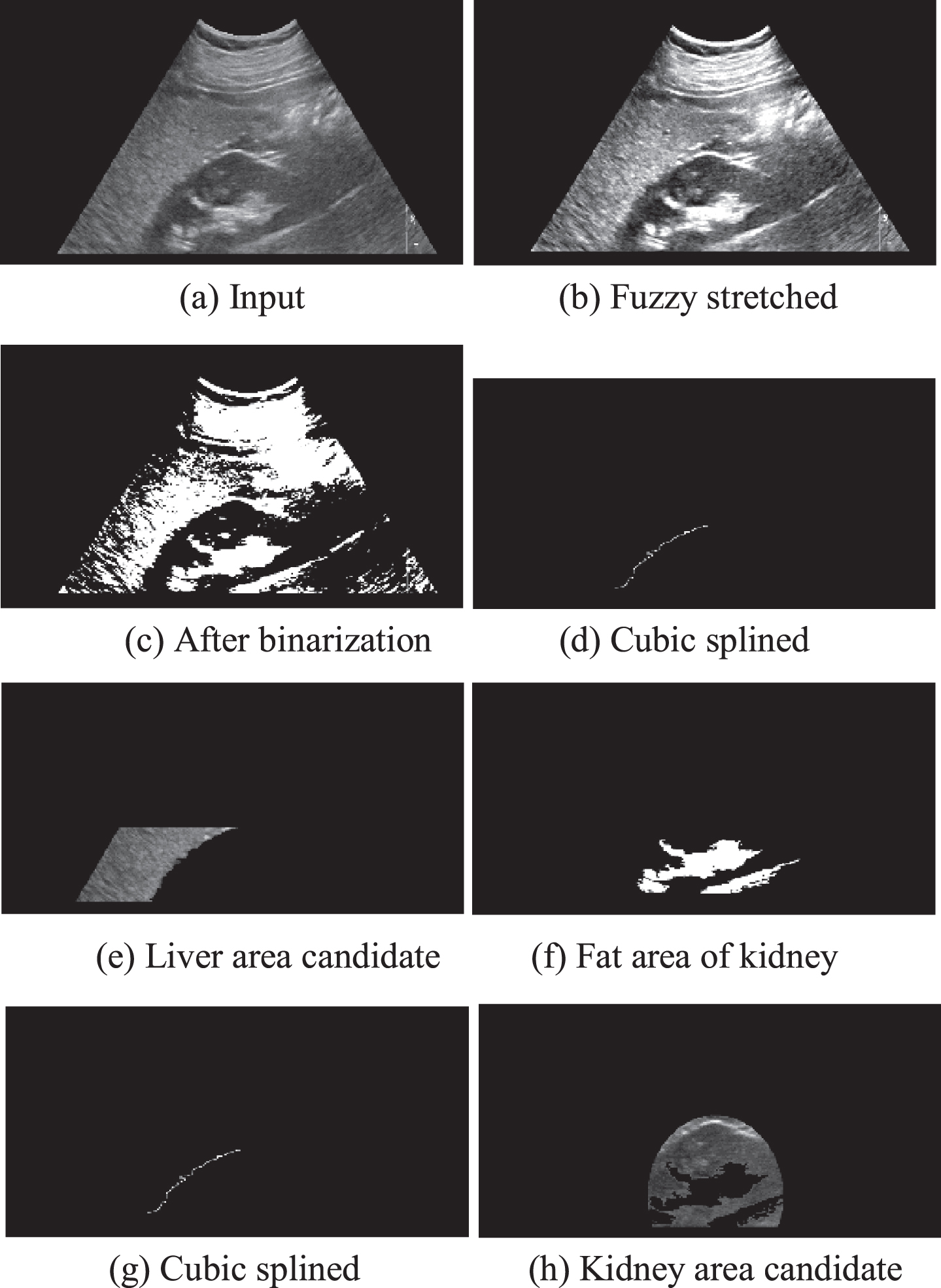
A typical ultrasound image containing the liver and the right kidney areas has relatively low intensity. There exists a limiting membrane with a high intensity as the border of our two ROIs—the liver and the right kidney. The first major step of image preprocessing for this analysis is to enhance the brightness contrast. The ultrasound image contains a relatively bright area such as abdomen muscles, fascia, fat area in the kidney, and the border lines between the liver and the kidney. We apply the dynamic fuzzy stretching technique [19] to enhance the contrast by dynamically controlling the maximum and the minimum range of the stretching with a triangle-type fuzzy membership function. Then, the average binarization technique is applied to extract fat area of the kidney part. Then the 8-directional contour tracking algorithm [48] is applied for object formation as explained in [19]. Knowing that relatively brighter muscles of abdomen and fascia exist at upper part of the image, our search is confined to the lower part of the image. Since such edge tracking may have small disconnections during the object labeling process, we apply monotone cubic spline [49] to reconnect the related objects to complete the boundary lines. The details of such interpolation process can be found in [50].
Figure 1 summarizes our preprocessing steps. The edge tracking algorithm tracks pixels having the same object label. Cubic spline interpolation forms the boundary lines between the liver and kidney and then the object formation algorithms are applied to the left (liver) and right (kidney) of the splined line as shown in Fig. 1(e) and (h) respectively.
Fig. 1
Image preprocessing for target object extractions.
2.2DFCM algorithm
FCM clustering [37] is an unsupervised clustering technique applied to segmenting images into clusters with similar spectral properties. It utilizes the distance between pixels and cluster centers in the spectral domain to compute the membership. The cost function is minimized when pixels close to the centroid of their clusters are assigned higher membership values, and the farther the data point is from the centroid, the lower the assigned membership values are. The membership function represents the probability that a pixel belongs to a specific cluster. In the FCM algorithm, the probability is dependent solely on the distance between the pixel and each individual cluster center in the feature domain.
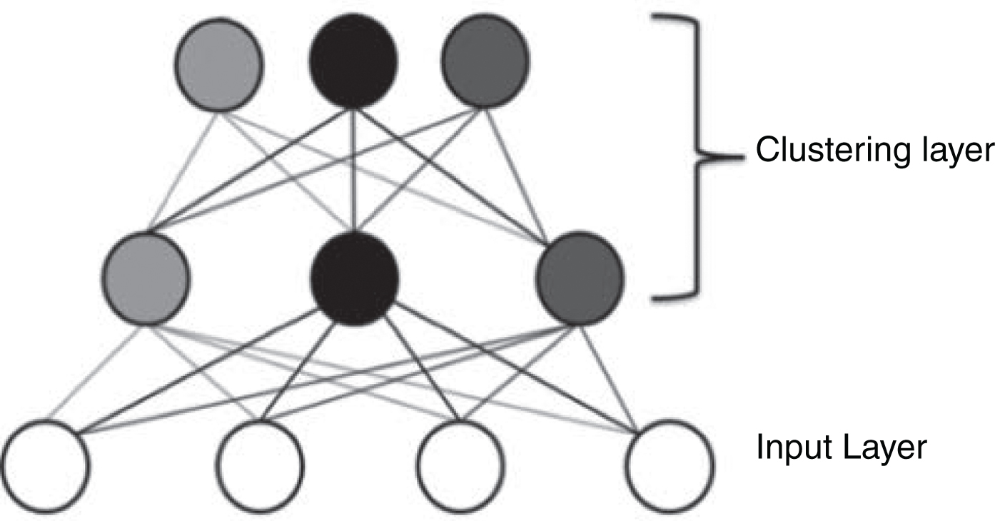
FCM usually could not minimize the intra-cluster variance and could not maximize the inter-cluster variance due to the overlapping of regions and/or the sensitivity to the outlier. Also, because of using the gradient descent method, it can be easily fallen into local optimal solutions and cannot gain the global optimal solution. In this paper, we try to avoid such local maxima problem by applying double-layered learning for FCM. By doing so, our DFCM can pursuit the global optimization of the cost function effectively. The concept of DFCM can be shown in Fig. 2.
Fig. 2
Double-layered learning structure.
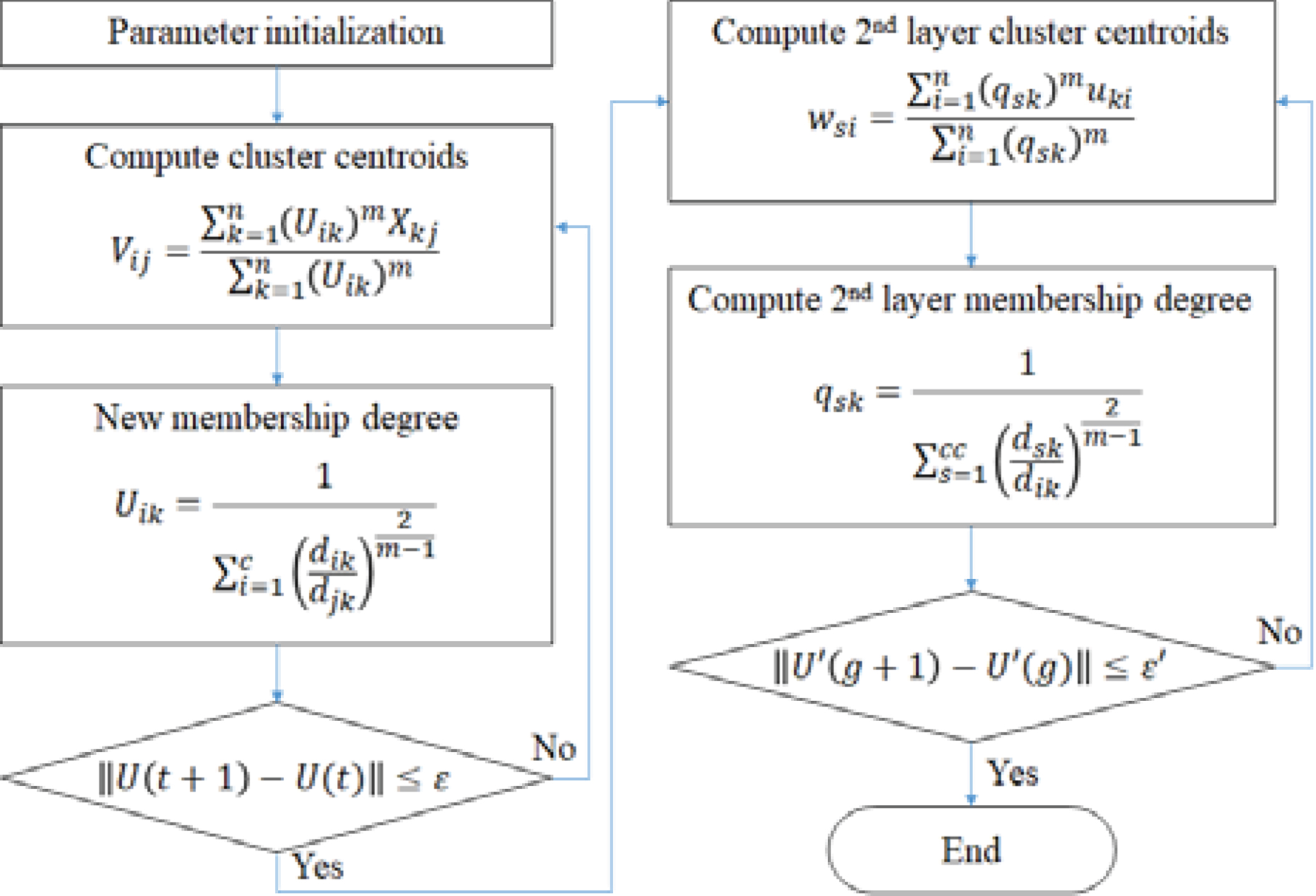
Then the DFCM quantization is done as following;
Step 1: Initialize c (2≤c< n) as the number of clusters, and exponential weight m (1≤m< ∞). Also initialize the error threshold (ɛ) for terminating condition of the first layer learning and the membership degree U(0).
Step 2: Compute the value of central vector Vij as shown in Equation (1) for vi | i = 1, 2, ... , c.
(1)
Step 3: Define the FCM cost function J as Equation (2).
(2)
In order to minimize J, dik and membership function U are defined as Equation (3) and (4), respectively.
(3)
(4)
Step 4: Compute the difference (Uik(r + 1)-Uik(r)) between the new membership and the previous membership degree at the time of r. If the difference is less than the error threshold (ɛ), then the algorithm goes to Step 5, otherwise go to Step 2.
Step 5: With output of the first layer as the input of the second layer, compute the value of central vector wsi as shown in Equation (5) for ws | s = 1, 2, ... , cc where cc is the number of clusters for the second layer.
(5)
Step 6: Compute the membership degree of the clusters qsk in the second layer with distance function dsk as Equation (6) and (7) respectively.
(6)
(7)
Step 7: Compute the difference between the new membership and the previous membership degree. If the difference is less than the final error threshold (ɛ’), then the algorithm terminates otherwise go to Step 5.
This process can be summarized as Fig. 3.
Fig. 3
Double-layered FCM algorithm.
2.3HRI computation and visual representation
The effect of DFCM for the final liver/kidney area extraction can be shown as Fig. 4.
Fig. 4
Final area extractions.
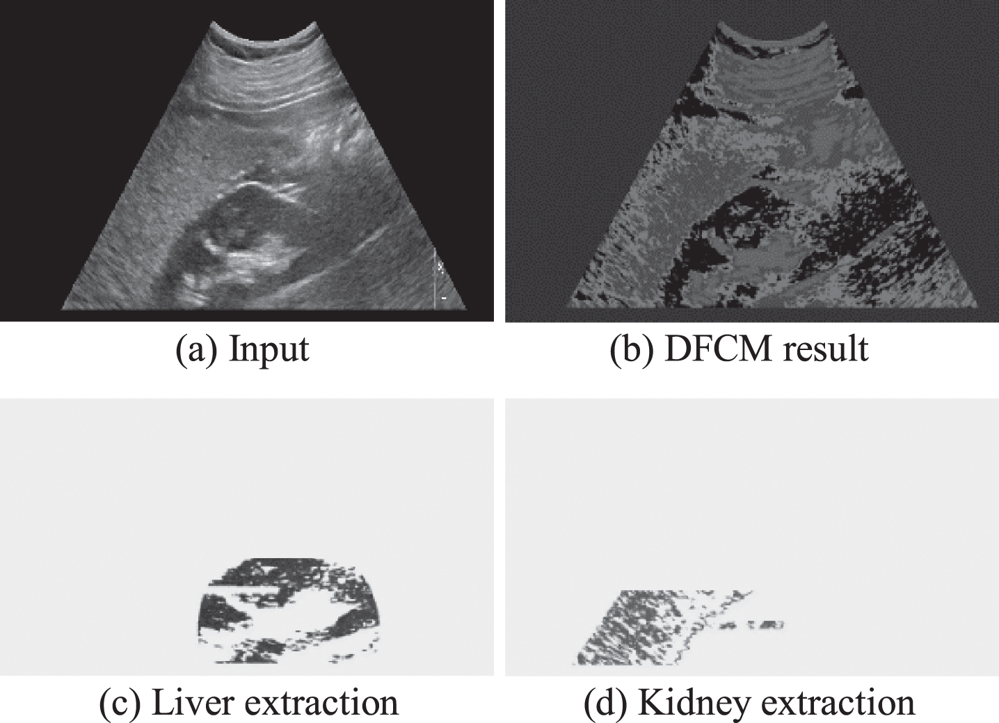
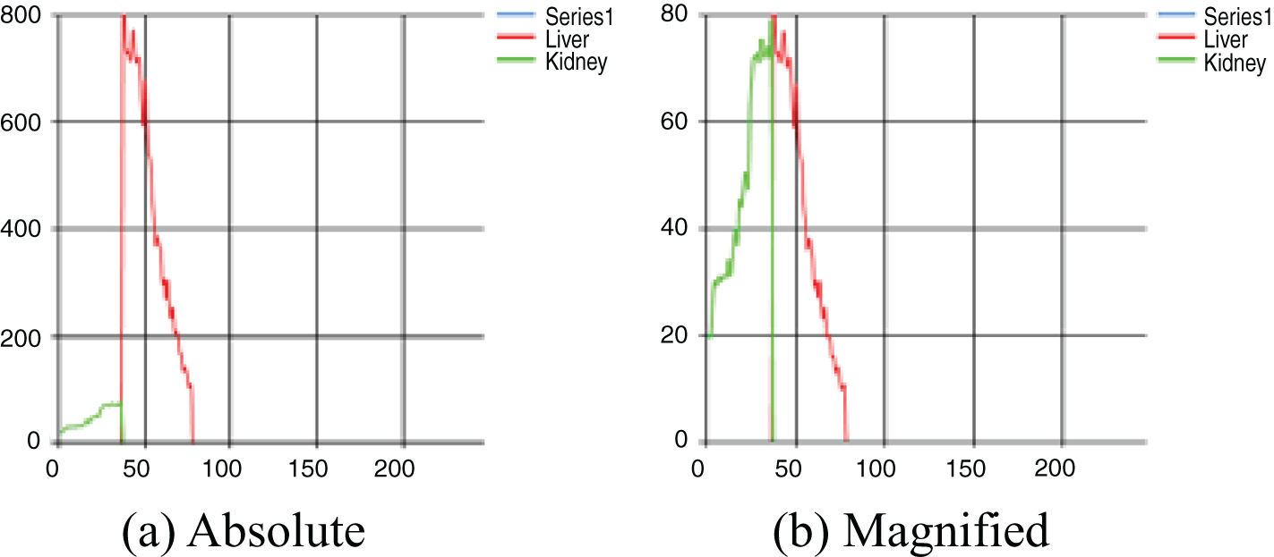
The HRI is computed as the rate of liver echogenicity to that of the right kidney cortex. Since we use pixel clustering strategy, the distribution of echogenicity can be shown in Fig. 5(a) but the kidney part can be magnified as shown in Fig. 5(b) in order to compare the distribution visually only for the radiologists’ convenience. The X-axis represents the echogenicity and the y-axis represents the frequency of pixels in the extracted object area. The average of liver echogenicity is divided by the average echogenicity of kidney area to determine the HRI.
Fig. 5
Visual representation of echogenicity.
3The utility of HRI and distribution shape variables: Experiment and analysis
The proposed method is implemented in Visual Studio 2017 C# with AMD Ryzen 5 1400 Quad-core processor of 3.20 GHz and 8.00GB RAM PC. 50 subjects aged 18 or more who finished a health checkup with abdominal ultrasonography as a screening examination at Pusan National University Hospital in Korea in 2017 participated in this experiment. Images were obtained by the right subcostal scan including the lower pole of the liver and the right kidney. Obtained ultrasonographic images are of the 1024×768 bitmap format with 5 MHz in probing and the machine was produced by Phillips with software version PMS5.1 Ultrasound iU22_5.2.0.289. No subject participated in this experiment reported prior surgical experience of liver or kidney.
Three radiologists are participated in reviewing and evaluating the severity stage of NAFLD of those 50 ultrasonographic images without any information from the proposed software thus the ground truth of severity stage of this experiment is decided by the majority voting of three radiologists. Table 1 summarizes the severity stage of 50 subjects evaluated by three radiologists.
Table 1
Severity of NAFLD stage in this experiment: the ground truths
| Stage | Unanimous | Split | Total |
| Normal | 21 | 3 | 24 |
| Mild | 8 | 4 | 12 |
| Moderate | 3 | 8 | 11 |
| Severe | 3 | 0 | 3 |
| Total | 35 | 15 | 50 |
As represented in Table 1, the rate of unanimous decisions of three participated radiologists are only 70% and the intra-class correlation coefficient of their decision is computed as 0.673 that is “good” by the standard of [51].
Intra class correlation coefficient (ICC) is defined as Equation (8).
(8)
For the evaluation of the severity stage of NAFLD from ultrasound images, the proposed software provides HRI rate and three other useful statistics of characterizing the echogenicity distribution – skewness, kurtosis, and CV of the liver echogenicity. Skewness is a measure of the asymmetry of the distribution of a variable. The skew value of a normal distribution is zero, usually implying symmetric distribution. A positive skew value indicates that the tail on the right side of the distribution is longer than the left side and the bulk of the values lie to the left of the mean. In contrast, a negative skew value indicates that the tail on the left side of the distribution is longer than the right side and the bulk of the values lie to the right of the mean. Kurtosis is a measure of the peak of a distribution [52]. Distributions with negative kurtosis is called as platykurtic such that the distribution produces fewer and less extreme outliers than does the normal distribution. Distributions with positive kurtosis is called as leptokurtic, which has tails that asymptotically approach zero more slowly than normal distribution. CV, known as relative standard deviation, is a standardized measure of dispersion of a probability distribution or frequency distribution. It is often expressed as a percentage, and is defined as the ratio of the standard deviation to the mean. These three distribution statistics can explain the echogenicity distribution of the subject’s image as shown in Fig. 5 and may contribute to discriminate the severity stage of NAFLD. In fact, a recent research reported a decent accuracy of detecting and grading fatty liver disease by kurtosis based scanning method [53]. Table 2 summarizes the echogenicity values and distribution statistics generated by the proposed method.
Table 2
Echogenicity and Distribution Statistics by proposed DFCM. (*p<0.05, **p<0.01)
| Stage | HRI | Kurtosis | Skew ness | CV-Liver | Liver Echo | Kidney Echo |
| Normal | 1.06±0.13 | –0.53±0.67 | 0.44±0.39 | 4.56±0.82 | 50.32±7.26 | 48.04±7.06 |
| Mild | 1.32±0.18** | –0.69±0.30 | –0.01±0.47** | 6.96±2.67 | 69.49±16.28** | 52.72±10.53 |
| Moderate | 1.54±0.30* | –0.98±0.27** | 0.08±0.14 | 9.63±4.62 | 82.57±19.18 | 53.60±8.87 |
| Severe | 1.57±0.30 | –0.91±0.31 | 0.00±0.12 | 13.79±5.77 | 125.17±31.33 | 79.67±14.91 |
| Normal | 1.06±0.13 | –0.53±0.67 | 0.44±0.39 | 4.56±0.82 | 50.32±7.26 | 48.04±7.06 |
| Abnormal | 1.44±0.27** | –0.84±0.28** | 0.03±0.33** | 7.56±3.72** | 81.45±25.32** | 56.20±13.15* |
For each cell of Table 2, the first number is the mean and the second number is the standard deviation of each statistics of the same stage. We take t-test to each adjacent stages and double asterisk (**) denotes p < 0.01 and the single asterisk (*) denotes p < 0.05 otherwise two adjacent stages have no statistical difference. The bottom row ‘Abnormal’ means all stages other than normal. Two t-test results are shown in Table 2 in that the first t-test is to see if any variable is statistically different in any of 4 severity stage level (first 4 rows) and the second one is the t-test for normal/abnormal distinctions(bottom two rows). In this regard, all statistics by DFCM based segmentation are significant in discriminating normal stage from abnormal stage. However, in discriminating mild stage from moderate stage, the kurtosis is stronger variable than HRI. Liver echogenicity and the skewness are also significant in normal-mild stage discrimination. There exists no significant variable in discriminating moderate and severe stage. This might be due to the limited number of data for severe stage of NAFLD in this experiment.
In reviewing the data, the normal-abnormal cutoff value of HRI would be 1.30 that contains all normal cases under the cutoff. However, there is no single standard cutoff value of a variable appeared in Table 2. Interesting point is that the correlation of the kurtosis and HRI is extremely low (-0.02) thus it suggests that some combination of these two variables may be better decision making standard than depending on any one variable.
In order to see if the proposed DFCM itself produces better statistical measurements; we compare this result with SOM based pixel clustering [19] as a referendum since both have similar mechanisms in extracting liver/kidney area extractions automatically. Table 3 summarizes the echogenicity values and distribution statistics generated by the SOM based method.
Table 3
Echogenicity and Distribution Statistics by SOM [19]. (* p < 0.05, ** p < 0.01)
| Stage | HRI | Kurtosis | Skew ness | CV-Liver | Liver Echo | Kidney Echo |
| Normal | 1.03±0.24 | –0.89±0.31 | 0.18±0.29 | 7.29±2.56 | 45.72±8.31 | 45.98±9.94 |
| Mild | 1.41±0.72 | –0.94±0.20 | –0.08±0.27 | 10.20±5.41 | 63.85±19.31** | 51.19±18.27 |
| moderate | 1.50±0.44 | –0.89±0.33 | 0.08±0.32 | 6.51±2.51 | 79.06±21.87 | 54.97±16.64 |
| Severe | 1.92±0.31* | –1.00±0.04 | –0.05±0.02* | 25.97±4.46 | 129.09±21.47 | 69.53±23.23 |
| Normal | 1.03±0.24 | –0.89±0.31 | 0.18±0.29 | 4.56±0.82 | 45.72±8.31 | 45.98±9.94 |
| Abnormal | 1.51±0.58** | –0.93±0.25 | 0.02±0.29 | 11.78±7.10** | 77.81±28.73** | 54.91±18.25* |
SOM based method is successful on HRI for normal-abnormal discrimination. However, for severity stage classification, there is no statistically significant variable to discriminate mild and moderate stage. Thus, the proposed DFCM is better clustering algorithm to produce meaningful statistics for NAFLD severity stage classification.
Pixel echogenicity distribution and its characteristic attributes (skewness, kurtosis, CV) may be valuable statistics for stage classification although no single variable is as powerful as HRI. In Fig. 6, we demonstrate typical liver-kidney echogenicity.
Fig. 6
Typical examples of echogenicity distribution with respect to the severity stage.
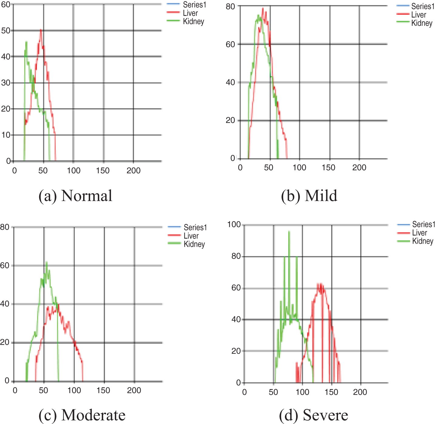
While radiologists make decisions of fatty liver severity level with quantified value (HRI) and qualitative measurement like graphs shown in Fig. 6, it is still very subjective as we have seen that the gold standard measured by multiple radiologists have only 70% of unanimous decisions on severity stage identification as shown in Table 1. Furthermore, although shape variables of the intensity distribution have statistically significant contributions in severity stage determination as shown in Table 2, there is no clear way to explain it in our post-hoc analysis. Thus, we try to find a set of decision rules for stage classification that can explain at least our limited 50 cases. Since we have only 3 ‘severe’ cases in our data set, it is not reliable to test any set of rules in standard machine learning paradigm. Rather, we want to see if there exists a good simple intuitive set of rules that may explain the stage classifications.
Thus, we use a standard decision tree open source written in Python that ‘fits’ all of our data set meaning that the set of rules we found is only effective over our data. We choose decision tree algorithm since there is a simple way to construct a set of rules from the tree structure by tracking every leaf node [54]. The tree that fits all 50 data is shown in Fig. 7 and the set of decision rules are formed as in Table 4.
Fig. 7
Decision tree to decide fatty liver severity classification.
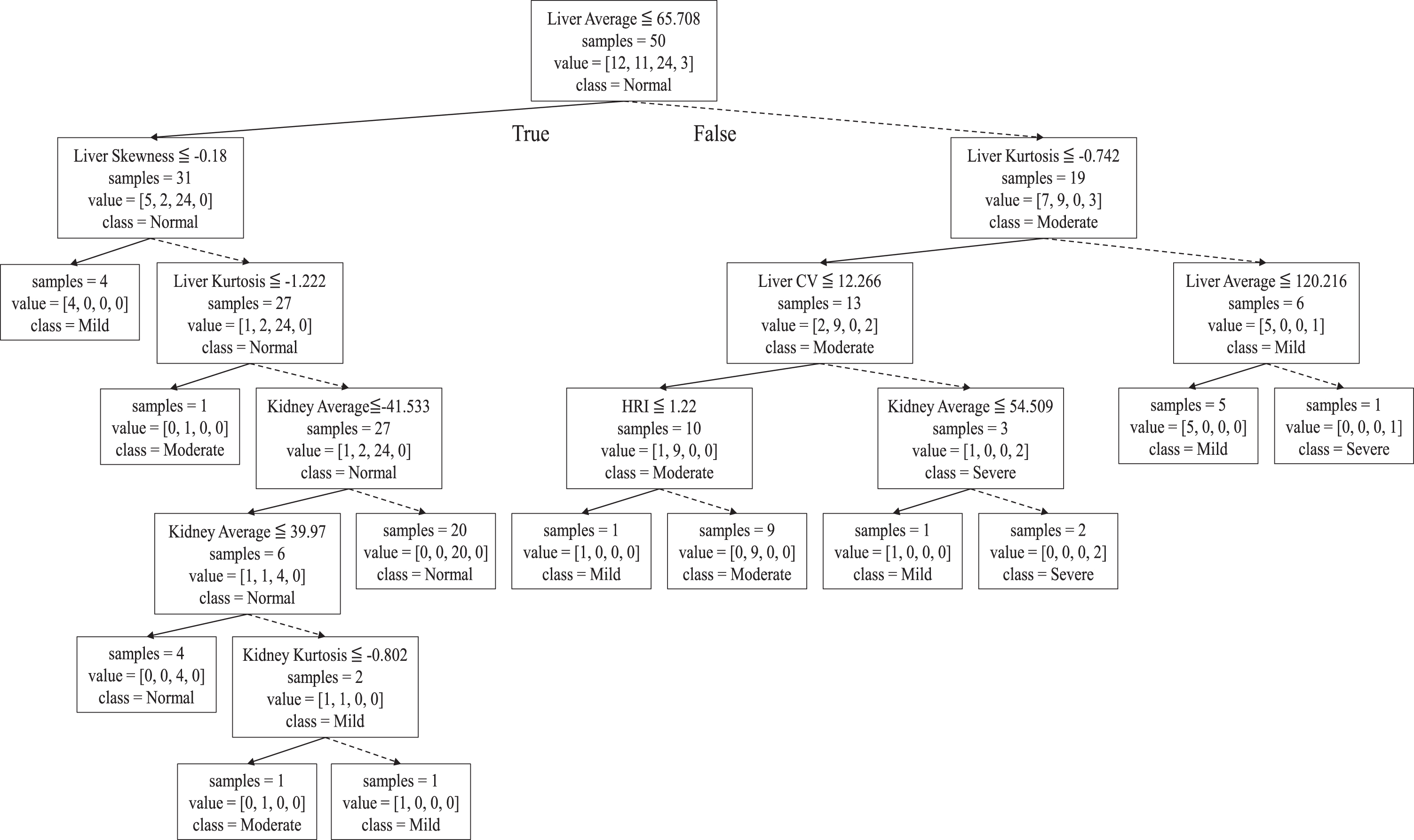
Table 4
Decision rules for fatty liver severity stage from decision tree of Fig. 7
| Stage | Data | Liver-Echo | Skewness | Kurtosis | Kidney-Echo | HRI | CV-Liver |
| Normal | 20 | ≦ 65.708 | >0.18 | ≦ -1.222 | >41.533 | ||
| Normal | 4 | ≦ 39.97 | >0.18 | ≦ -1.222 | ≦ 41.533 | ||
| Mild | 5 | [65.708, 120.216] | >0.742 | ||||
| Mild | 4 | ≦ 65.708 | ≦ -0.18 | ||||
| Mild | 1 | [39.97, 65.708] | >0.18 | ≦ -1.222 | ≦ 41.533 | >1.15 | |
| Mild | 1 | [65.708, 69.634] | ≦ -0.742 | ≦ 12.266 | |||
| Mild | 1 | [65.708, 79.912] | ≦ -0.742 | >12.266 | |||
| Moderate | 9 | >69.634 | ≦ -0.742 | ≦ 12.266 | |||
| Moderate | 1 | ≦ 65.708 | >0.18 | ≦ -1.222 | |||
| Moderate | 1 | [39.97, 65.708] | >0.18 | ≦ -1.222 | ≦ 41.533 | ≦ 1.15 | |
| Severe | 2 | >79.912 | ≦ -0.742 | >12.266 | |||
| Severe | 1 | >120.216 | >0.742 | ||||
| Total | 50 |
In Fig. 7, one can follow how the decision tree is formed. There are 24 normal, 12 mild, 11 moderate, and 3 severe stage people in our data set. A node represents four types of information in that the first row specifies the branching condition, the second row denotes current size of the set and the third row represents the distribution of data in this node as the order of [mild, moderate, normal, severe] (e.g. value = [3, 11, 12, 24] in the root node of Fig. 7) and the bottom row represents the majority class of the node. The classification is done at each leaf node in that all data in that node have the same class.
In Table 4, each row represents a rule that decides the stage (first column) with at most 6 possible independent variables satisfy the tests. Blank in the condition field (from 3rd to 8th column) means ‘don’t care’. The second column in each row denotes the number of data classified by that rule in our data set. Some examples of constructed rules are read as the following;
Rule 3: If the Liver-Echo is in interval [65.708, 120.216] and Kurtosis > 0.742, then the stage class would be ‘mild’ and 5 cases of our data belong to this rule.
... .
Rule 8: If the Liver-Echo> 69.634 and Kurtosis< =0.742 and CV of the Liver< =12.266 then the stage class would be ‘moderate’ and 9 cases of our data belong to this rule.
Surprisingly, we find that HRI is not the most decisive variable in severity stage classification while it was effective in normal/abnormal decision making. The Liver-Echo value and the Kurtosis of Liver intensity distribution play more important role instead. However, numbers given as branching conditions are not intuitive.
Thus, we verify that the severity classification is a challenging task and we need better set of features that can decide the stage classification as well as better, more reliable classification algorithm in this multi-class learning problem. Recent deep-learning based architectures [55–57] might have better classification power but they do not have sufficient explanative power of their decision making thus more researches are needed in this domain.
4Conclusion
In this paper, we develop a new automatic segmentation algorithm for Liver/Kidney area segmentation based on fuzzy C-means principle. Our DFCM quantization method overcomes the fixed initialization problem of the original FCM which frequently falls into local minimum in the processing and DFCM produces statistically better set of variables for fatty liver abnormality classification than previously proposed SOM based method. The distinction between normal and abnormalities is important in diagnosing fatty liver, but considering the clinical significance, the diagnosis of severity stage is more important. For this 4-class classification problem, simple single HRI cutoff does not work properly. We show that variables related with the shape of the intensity distribution of the ultrasonography are also as statistically significant as HRI in discriminating normal/abnormal fatty liver classification problem. In the severity stage classification, we show that these distribution shape related variables such as the kurtosis and the skewness of the liver intensity are more discriminative than HRI in this severity stage classification based on our rule construction result from decision tree principle.
The proposed DFCM method for segmentation and automatic quantification of HRI generate more statistically distinctive shape variables of intensity distribution in diagnosing severity stages of mild, moderate and severe classes of fatty liver than single HRI cutoff strategy. However, the limitation of this research is that the sample data size is only 50 in this 4-class classification and there were only 3 ‘severe’ stage data due to the data collection method (regular health checkup data) thus the result of this paper needs proof of the possibility of actual application through clinical research in the future.
Acknowledgments
This work was supported by a 2-Year Research Grant of Pusan National University. This research was conducted in a retrospective study, using only anonymizing ultrasonographic data and exempting patients’ consents from IRB (Institutional Review Board).
References
[1] | Younossi Z. , Anstee Q.M. , Marietti M. , Hardy T. , Henry L. , Eslam M. , George J. and Bugianesi E. , Global burden of NAFLD and NASH: trends, predictions, risk factors and prevention, Nature reviews Gastroenterology & Hepatology 15: ((2018) ), 11–20. |
[2] | Takahashi Y. and Fukusato T. , Histopathology of nonalcoholic fatty liver disease/nonalcoholic steatohepatitis, World Journal of Gastroenterology 20: ((2014) ), 15539. |
[3] | Amarapurkar D.N. , Hashimoto E. , Lesmana L.A. , Sollano J.D. , Chen P.J. and Goh K.L. , Asia–Pacific Working Party on NAFLD1, How common is non-alcoholic fatty liver disease in the Asia–Pacific region and are there local differences? Journal of Gastroenterology and Hepatology 22: ((2007) ), 788–793. |
[4] | Kwon Y. , Oh S. , Hwang S. , Lee C. , Kwon H. and Goh E.C. , Association of nonalcoholic fatty liver disease with components of metabolic syndrome according to body mass index in Korean adults, The American Journal of Gastroenterology 107: ((2012) ), 1852–1858. |
[5] | Wong V.W.S. , Wong G.L.H. , Choi P.C.L. , Chan A.W.H. , Li M.K.P. , Chan H.Y. , Chim A.M.L. , Yu J. , Sung J.J.Y. and Chan H.L.Y. , Disease progression of non-alcoholic fatty liver disease: a prospective study with paired liver biopsies at 3 years, Gut 59: ((2010) ), 969–974. |
[6] | Chalasani N. , Younossi Z. , Lavine J.E. , Diehl A.M. , Brunt E.M. , Cusi K. , Charlton M. and Sanyal A.J. , The diagnosis and management of non-alcoholic fatty liver disease: Practice Guideline by the American Association for the Study of Liver Diseases, American College of Gastroenterology, and the American Gastroenterological Association, Hepatology 55: ((2023) ), 2005–2023. |
[7] | Sung K.C. and Kim S.H. , Interrelationship between fatty liver and insulin resistance in the development of type 2 diabetes, The Journal of Clinical Endocrinology & Metabolism 96: ((2011) ), 1093–1097. |
[8] | Musso G. , Gambino R. , Cassader M. and Pagano G. , Meta-analysis: natural history of non-alcoholic fatty liver disease (NAFLD) and diagnostic accuracy of non-invasive tests for liver disease severity, Annals of Medicine 43: ((2011) ), 617–649. |
[9] | Saverymuttu S.H. , Joseph A.E. and Maxwell J.D. , Ultrasound scanning in the detection of hepatic fibrosis and steatosis, Br Med J (Clin Res Ed) 292: ((1986) ), 13–15. |
[10] | Mustapic S. , Ziga S. , Matic V. , Bokun T. , Radic B. , Lucijanic M. , Marusic S. , Babic Z. and Grgurevic I. , Ultrasound grade of liver steatosis is independently associated with the risk of metabolic syndrome, Canadian Journal of Gastroenterology and Hepatology 2018 (2018). |
[11] | Ratziu V. , Charlotte F. , Heurtier A. , Gombert S. , Giral P. , Bruckert E. , Grimaldi A. , Capron F. and Poynard T. , LIDO Study Group, Sampling variability of liver biopsy in nonalcoholic fatty liver disease, Gastroenterology 128: ((2005) ), 1898–1906. |
[12] | Zelber-Sagi S. , Webb M. , Assy N. , Blendis L. , Yeshua H. , Leshno M. , Ratziu V. , Halpern Z. , Oren R. and Santo E. , Comparison of fatty liver index with noninvasive methods for steatosis detection and quantification, World Journal of Gastroenterology 19: ((2013) ), 57. |
[13] | Lall C.G. , Aisen A.M. , Bansal N. and Sandrasegaran K. , Nonalcoholic fatty liver disease, American Journal of Roentgenology 190: ((2008) ), 993–1002. |
[14] | Xia M.F. , Yan H.M. , He W.Y. , Li X.M. , Li C.L. , Yao X.Z. , Li R.K. , Zeng M.S. and Gao X. , Standardized ultrasound hepatic/renal ratio and hepatic attenuation rate to quantify liver fat content: an improvement method, Obesity 20: ((2012) ), 444–452. |
[15] | Cengiz M. , Sentürk S. , Cetin B. , Bayrak A.H. and Bilek S.U. , Sonographic assessment of fatty liver: intraobserver and interobserver variability, International Journal of Clinical and Experimental Medicine 7: ((2014) ), 5453. |
[16] | Sabih D. and Hussain M. , Automated classification of liver disorders using ultrasound images, Journal of Medical Systems 36: ((2012) ), 3163–3172. |
[17] | Krishnan K.R. and Sudhakar R. , Automatic classification of liver diseases from ultrasound images using GLRLM texture features, In Soft Computing Applications (2013), 611–624. |
[18] | Neogi N. , Adhikari A. and Roy M. , Classification of ultrasonography images of human fatty and normal livers using GLCM textural features, Current Trends in Technology and Science 3: ((2014) ), 252–259. |
[19] | Kim K.B. and Kim C.W. , Quantification of hepatorenal index for computer-aided fatty liver classification with self-organizing map and fuzzy stretching from ultrasonography, BioMed Research International 2015 (2015). |
[20] | Acharya U.R. , Sree S.V. , Ribeiro R. , Krishnamurthi G. , Marinho R.T. , Sanches J. and Suri J.S. , Data mining framework for fatty liver disease classification in ultrasound: a hybrid feature extraction paradigm, Medical Physics 39: ((2012) ), 4255–4264. |
[21] | Singh M. , Singh S. and Gupta S. , An information fusion based method for liver classification using texture analysis of ultrasound images, Information Fusion 19: ((2014) ), 91–96. |
[22] | Li S. , Jiang H. , Yao Y.D. and Yang B. , Organ location determination and contour sparse representation for multiorgan segmentation, IEEE Journal of Biomedical and Health Informatics 22: (3) ((2017) ), 852–861. |
[23] | Al-Shaikhli S.D.S. , Yang M.Y. and Rosenhahn B. , Automatic 3D liver segmentation using sparse representation of global and local image information via level set formulation. arXiv preprint arXiv:1508.01521. (2015). |
[24] | Bharti P. , Mittal D. and Ananthasivan R. , Computer-aided characterization and diagnosis of diffuse liver diseases based on ultrasound imaging: a review, Ultrasonic Imaging 39: ((2017) ), 33–61. |
[25] | Targher G. , Bertolini L. , Rodella S. , Lippi G. , Zoppini G. and Chonchol M. , Relationship between kidney function and liver histology in subjects with nonalcoholic steatohepatitis, Clinical Journal of the American Society of Nephrology 5: ((2010) ), 2166–2171. |
[26] | Park Y.S. , Lee C.H. , Choi K.M. , Lee J. , Choi J.W. , Kim K.A. and Park C.M. , Correlation between Abdominal Fat Amount and Fatty Liver, using Liver to Kidney Echo Ratio on Ultrasound, Ultrasonography 31: ((2012) ), 219–224. |
[27] | İçer S. , Coşkun A. and İkizceli T. , Quantitative grading using grey relational analysis on ultrasonographic images of a fatty liver, Journal of Medical Systems 36: ((2012) ), 2521–2528. |
[28] | Hernaez R. , Lazo M. , Bonekamp S. , Kamel I. , Brancati F.L. , Guallar E. and Clark J.M. , Diagnostic accuracy and reliability of ultrasonography for the detection of fatty liver: a meta-analysis, Hepatology 54: ((2011) ), 1082–1090. |
[29] | Webb M. , Yeshua H. , Zelber-Sagi S. , Santo E. , Brazowski E. , Halpern Z. and Oren R. , Diagnostic value of a computerized hepatorenal index for sonographic quantification of liver steatosis, American Journal of Roentgenology 192: ((2009) ), 909–914. |
[30] | Shiralkar K. , Johnson S. , Bluth E.I. , Marshall R.H. , Dornelles A. and Gulotta P.M. , Improved method for calculating hepatic steatosis using the hepatorenal index, Journal of Ultrasound in Medicine 34: ((2015) ), 1051–1059. |
[31] | Marshall R.H. , Eissa M. , Bluth E.I. , Gulotta P.M. and Davis N.K. , Hepatorenal index as an accurate, simple, and effective tool in screening for steatosis, American Journal of Roentgenology 199: ((2012) ), 997–1002. |
[32] | Chauhan A. , Sultan L.R. , Furth E.E. , Jones L.P. , Khungar V. and Sehgal C.M. , Diagnostic accuracy of hepatorenal index in the detection and grading of hepatic steatosis, Journal of Clinical Ultrasound 44: ((2016) ), 580–586. |
[33] | von Volkmann H.L. , Havre R.F. , Løberg E.M. , Haaland T. , Immervoll H. , Haukeland J.W. , Hausken T. and Gilja O.H. , Quantitative measurement of ultrasound attenuation and hepato-renal index in non-alcoholic fatty liver disease, Medical Ultrasonography 15: ((2013) ), 16–22. |
[34] | Lee Y.C. , Wu J.S. , Yang Y.C. , Chang C.S. , Lu F.H. and Chang C.J. , Moderate to severe, but not mild, nonalcoholic fatty liver disease associated with increased risk of gallstone disease, Scandinavian Journal of Gastroenterology 49: ((2014) ), 1001–1006. |
[35] | Targher G. , Byrne C.D. , Lonardo A. , Zoppini G. and Barbui C. , Non-alcoholic fatty liver disease and risk of incident cardiovascular disease: a meta-analysis, Journal of Hepatology 65: ((2016) ), 589–600. |
[36] | Siddiqui M.S. , Fuchs M. , Idowu M.O. , Luketic V.A. , Boyett S. , Sargeant C. , Stravitz R.T. , Puri P. , Matherly S. , Sterling R.K. , Contos M. and Sanyal A.J. , Severity of nonalcoholic fatty liver disease and progression to cirrhosis are associated with atherogenic lipoprotein profile, Clinical Gastroenterology and Hepatology 13: ((2015) ), 1000–1008. |
[37] | Bezdek J.C. , Pattern recognition with fuzzy objective function algorithms. Springer Science & Business Media (2013). |
[38] | Li K. , Zhang C. , Chen Z. and Chen Y. , Development of a weighted fuzzy c-means clustering algorithm based on JADE, International Journal of Numerical Analysis and Modeling 5: ((2014) ), 113–122. |
[39] | Razavi M. , Wang L. , Gubern-Mérida A. , Ivanovska T. , Laue H. , Karssemeijer N. and Hahn H.K. , Towards accurate segmentation of fibroglandular tissue in breast MRI using fuzzy c-means and skin-folds removal, In International Conference on Image Analysis and Processing (2015), 528–536. |
[40] | Hassan M. , Chaudhry A. , Khan A. and Iftikhar M.A. , Robust information gain based fuzzy c-means clustering and classification of carotid artery ultrasound images, Computer Methods and Programs in Biomedicine 113: ((2014) ), 593–609. |
[41] | Hong J.S. , Kaneko T. , Sekiguchi R. and Park K.H. , Automatic liver tumor detection from CT, IEICE Transactions on Information and Systems 84: ((2001) ), 741–748. |
[42] | Kim K.B. , Song Y.S. , Park H.J. , Song D.H. and Choi B.K. , A fuzzy C-means quantization based automatic extraction of rotator cuff tendon tears from ultrasound images, Journal of Intelligent & Fuzzy Systems 35: ((2018) ), 149–158. |
[43] | Ceylan R. , Ceylan M. , Özbay Y. and Kara S. , Fuzzy clustering complex-valued neural network to diagnose cirrhosis disease, Expert Systems with Applications 38: ((2011) ), 9744–9751. |
[44] | Fu H. and Elmisery A.M. , A new feature weighted fuzzy c-means clustering algorithm, Algarve (2009), 11–18. |
[45] | Wu K.L. and Yang M.S. , Alternative c-means clustering algorithms, Pattern Recognition 35: ((2002) ), 2267–2278. |
[46] | Siddiqui F.U. , Isa N.A.M. and Yahya A. , Outlier rejection fuzzy c-means (ORFCM) algorithm for image segmentation, Turkish Journal of Electrical Engineering & Computer Sciences 21: ((2013) ). |
[47] | Kim K.B. , Song D.H. and Yun S.S. , Automatic extraction of blood flow area in brachial artery for suspicious hypertension patients from color doppler sonography with fuzzy C-means clustering, Journal of Information and Communication Convergence Engineering 16: ((2018) ), 258–263. |
[48] | Jess D.B. , Mathioudakis M. , Erdélyi R. , Verth G. , McAteer R.T.J. and Keenan F.P. , Discovery of spatial periodicities in a coronal loop using automated edge-tracking algorithms, The Astrophysical Journal 680: ((2008) ), 1523. |
[49] | Kanth A.S.V.R. and Reddy Y.N. , Cubic spline for a class of singular two-point boundary value problems, Applied Mathematics and Computation 170: ((2005) ), 733–740. |
[50] | Kim K.B. , Song D.H. and Kim C.W. , Automatic extraction of liver and kidney area from ultrasonography with contrast-enhanced image processing technique for correct fat liver analysis, Journal of Medical Imaging and Health Informatics 7: ((2017) ), 667–673. |
[51] | Cicchetti D.V. , Guidelines, criteria, and rules of thumb for evaluating normed and standardized assessment instruments in psychology, Psychological Assessment 6: ((1994) ), 284–290. |
[52] | Kim H.Y. , Statistical notes for clinical researchers: assessing normal distribution (2) using skewness and kurtosis, Restorative Dentistry & Endodontics 38: ((2013) ), 52–54. |
[53] | Ma H.Y. , Zhou Z. , Wu S. , Wan Y.L. and Tsui P.H. , A computer-aided diagnosis scheme for detection of fatty liverbased on ultrasound kurtosis imaging, Journal of Medical Systems 40: ((2016) ), 33. |
[54] | Quinlan J.R. , C4. 5: programs formachine learning. Elsevier (2014). |
[55] | Byra M. , Styczynski G. , Szmigielski C. , Kalinowski P. , Michałowski Ł. , Paluszkiewicz R. , Ziarkiewicz-Wróblewska B. , Zieniewicz K. , Sobieraj P. and Nowicki A. , Transfer learning with deep convolutional neural network for liver steatosis assessment in ultrasound images, International Journal of Computer Assisted Radiology and Surgery 13: ((2018) ), 1895–1903. |
[56] | Reddy D. , Santhosh R.B. and Rajalakshmi P. , Classification of Nonalcoholic Fatty Liver Texture Using Convolution Neural Networks, In 2018 IEEE 20th International Conference on e-Health Networking, Applications and Services (Healthcom) (2018), 1–5. |
[57] | Tajbakhsh N. , Shin J.Y. , Gurudu S.R. , Hurst R.T. , Kendall C.B. , Gotway M.B. and Liang J. , Convolutional neural networks for medical image analysis: Full training or fine tuning? IEEE Transactions on Medical Imaging 35: ((2016) ), 1299–1312. |


