
Fault diagnosis of high power grid wind turbine based on particle swarm optimization BP neural network during COVID-19 epidemic period
Abstract
During the COVID-19 pandemic, the maintenance of the wind turbine is unable to be processed due to the problem of personnel. This paper presents two neural network models: BP neural network and LSTM neural network combined with Particle Swarm Optimization (PSO) algorithm to realize obstacle maintenance detection for wind turbine. Aiming at the problem of gradient vanishing existing in the traditional regression neural network, a fault diagnosis model of wind turbine rolling bearing is proposed by using long-term and short-term memory neural network. Through the analysis of an example, it is verified that the diagnosis results of this method are consistent with the actual fault diagnosis results of wind turbine rolling bearing and the diagnosis accuracy is high. The results show that the proposed method can effectively diagnose the rolling bearing of wind turbine, and the long-term and short-term memory neural network still has good fault diagnosis performance when the difference of fault characteristics is not obvious, which shows the feasibility and effectiveness of the method.
1Introduction
In recent years, as a kind of green energy, wind energy plays an increasingly important role in the world energy structure. At the same time, wind power related equipment has also been rapid development. By 2020, the cumulative number of wind turbines in China is 192981 [1, 2], and the number of new wind turbines in 2020 is 16470 [3, 4]. The continuous increase of wind power related equipment brings a series of difficult problems to equipment maintenance personnel, such as the frequent occurrence of faults which makes the equipment maintenance cost gradually increase [5]. Among all kinds of faults of wind turbine, although the number of faults of transmission system is not the most, the downtime caused by faults is the longest [6].
Generally speaking, most fault diagnosis methods adopt the method of threshold discrimination. The main disadvantage of this method is that it is often difficult to objectively reflect the accurate law between faults and feature [7–11]. Artificial neural network, fuzzy theory, support vector machine and other intelligent diagnosis methods are applied to proposed model. However, with the development of its application, its limitations gradually appear, such as the possibility of falling into local optimal value, slow convergence speed of network, strong sample dependence and other defects [12–14]. This method has the advantages of gradient method and Newton method, so that the diagnostic accuracy of BP neural network is significantly improved, and the convergence speed of BP Neural Network (BPNN) is accelerated. However, this method not only improves some defects of the algorithm, but also increases the complexity of the algorithm.
Elman neural network is used to model bearing fault diagnosis, and the experiment shows that the performance of the proposed model is better than BPNN [15]. The performance of two kinds of neural networks, BPNN and recurrent Neural Network (NN), in fault diagnosis is fully compared, which shows that the recursive NN has a good improvement in convergence speed, accuracy of diagnosis results and algorithm stability compared with BPNN. Therefore, the recurrent NN has a good development potential in the field of fault diagnosis, but the traditional Recurrent NN (RNN) has its own shortcomings, for example, in the process of each feedback, some information will be lost. When time accumulates to a certain extent, the initial information will degenerate and the gradient vanishing effect will appear.
Based on the consideration of the coordination and complementarity of distributed energy and traditional voltage control equipment, this paper establishes multi-objective model for the cost, network loss, voltage offset and other indexes representing the stability and reliability of distribution network operation, and solves them with improved particle swarm optimization algorithm.
In view of the outstanding performance of recurrent NN in fault diagnosis, as well as the problems of traditional recurrent NN. In this paper, wavelet packet transform, short-term memory NN and particle algorithm are introduced into fault diagnosis of wind turbine bearing.
2Improvement of particle swarm optimization
2.1Limitation and improvement of algorithm
This is mainly due to the loss of diversity in the search space and the fact that the flight speed of particles cannot be adjusted according to the actual situation.
Most of the literatures [16–18] use the weight that decreases linearly with the number of iterations, but this kind of weight is not enough to solve the problem that particles are easy to fall into local optimum because of the linear convergence trend [19, 20]. It can be noted that:
(1)
The existence of factor λ can effectively overcome the defect that particles cannot jump out of the local area, and make particles converge rapidly. The position iteration formula with contraction factor λ is as follows:
(2)
The expression of λ is:
(3)
In the formula, φ= c1 + c2, in most literatures, φ ≥ 4.
Neighborhood learning can make the population keep better diversity, and the neighborhood particles of the learning target must be the most adaptive in the neighborhood. The improved speed iteration formula is as follows:
(4)
C3 is used as an acceleration factor to guide particles to learn from the optimal particles in the neighborhood, but the influence ability of the optimal neighborhood is less than that of pid and pgd, so c3 is lower than c1 and c2 in numerical selection.
PSO is the same as genetic algorithm, the quality of initial value will have a direct impact on the calculation speed, and the crossover operation in genetic algorithm can ensure the quality of initial value. In view of this, in genetic algorithm, applying the crossover stage of initial value selection to PSO algorithm will be beneficial to ensure the superiority of initial value of the algorithm. The following formula can be used for cross operation:
(5)
(6)
2.2Objective function
The economy of power system operation is of great significance to the benefit of enterprises and society. The network loss will affect the power supply quality of users and make the line overheat. Although the network loss cannot be completely eliminated, it can be reduced to a certain extent. In addition, the reduction of network loss plays an active role in protecting lines, reducing voltage drop and improving voltage level. Therefore, the objective problem is described as follows:
(1) The reasonable access of DG can improve the network loss of the system, so as to improve the economic operation of the distribution network. The established system network loss index is as follows:
(6)
Where, Ui and Uj are the voltage values of node i and node j respectively; Gij and θij are the conductance and voltage phase angle difference between node i and node j.
(2) Due to the access of some renewable energy, the voltage stability of the system will be affected to a certain extent. The voltage stability index is established as follows:
(7)
Where Uiref is the rated voltage of node i, Uimax and Uimin are the maximum and minimum voltage of node i respectively.
(3) The main cost of the active distribution network is the coal consumption of thermal power units and the operation and maintenance costs of capacitors and batteries. Therefore, the economic cost target is:
(9)
In the formula, CB is the power purchase cost; COP is the operation cost, mainly the operation and maintenance cost of the battery; CDEP is the depreciation cost; CL is the loss cost;
In this paper, voltage offset and cost can be set as the optimization objectives:
(10)
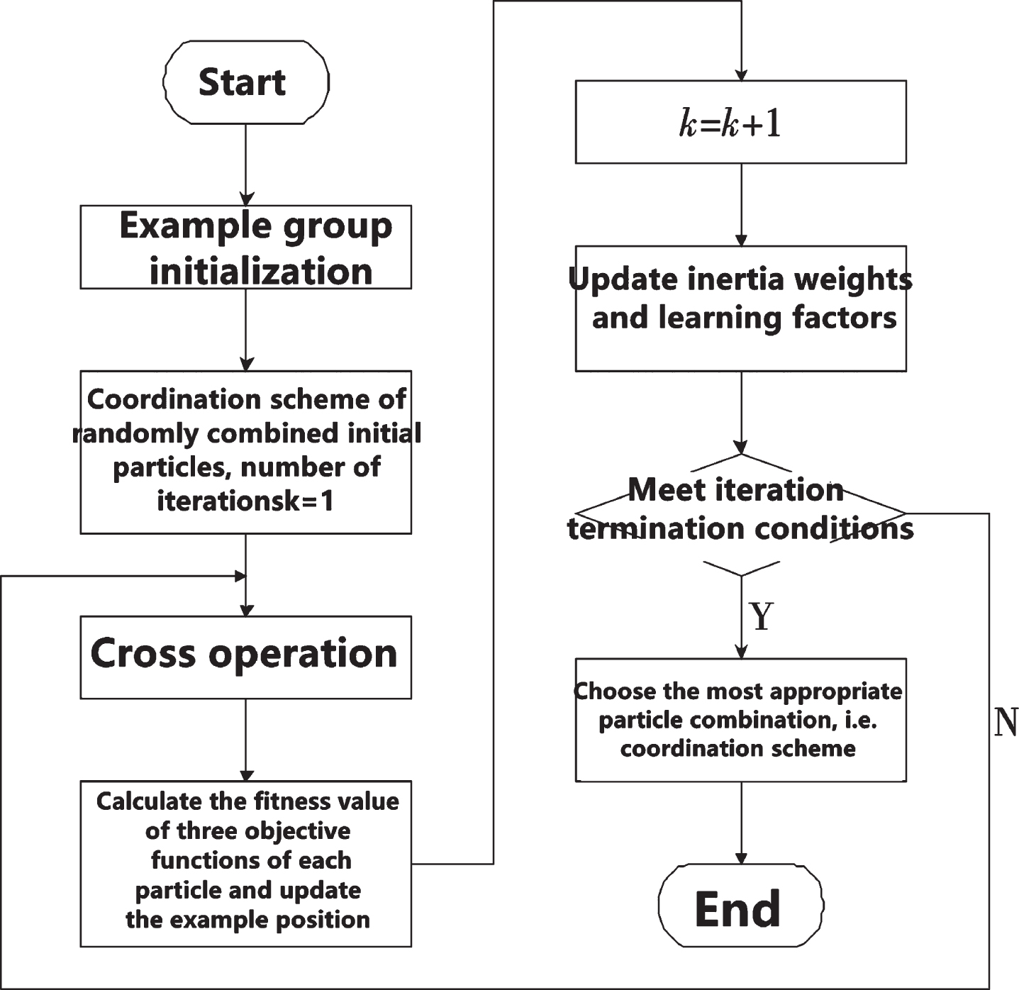
The algorithm flow is shown in Fig. 1.
Fig. 1
Algorithm flow.
3BPNN
3.1BPNN
The main idea of BP neural network algorithm is to divide the learning process of neural network into two stages: signal forward calculation and error back propagation. That is to say, for each sample data, it needs many forward calculation and back propagation to get the appropriate neural network model to fit the nonlinear relationship between input and output in the sample.
The neural network uses the existing data to find the weight relationship between input and output (approximate). Such a weight relation can be used for simulation, such as inputting a group of data to simulate the output results. At this time, the input is in the same category as the data set used in training. For example, weather forecast: temperature, humidity, air pressure, etc. are used as input and weather conditions are used as output. The neural network is trained by using the input-output relationship of history. Then the neural network is used to input the temperature, humidity and pressure of today to get the weather situation. Similarly, when applied to automated testing, test data can be used to reflect the trend of the results, the number of bugs, and quality problems, etc., which can also be predicted in advance.
Among many ANN models, BP (back propagation) network is more suitable for nonlinear fault prediction of complex mechanical equipment, and make a big difference in fault prediction of equipment or system.
Suppose an arbitrary network with L-layer and N nodes, given s samples (xk, dk) (k = 1, 2,…,S), the input sum of the j-th neuron in the L-th layer of the network is
(11)
(12)
In back propagation, the sum of the error square of the expected output dk and the actual output yk of the network is defined as the objective function, that is:
(13)
The total error of s samples is defined as:
(14)
The learning problem of the network is equivalent to the unconstrained optimization problem. By adjusting the weight W, the total error E is minimized, and the weight changes along the negative gradient direction of the error function, namely:
(15)
Where, t is the number of iterations; η is the step size.
Because the algorithm used in BPNN is based on the gradient descent of function, the algorithm is essentially a single point search algorithm and does not have the ability of global search. Therefore, there are some shortcomings in the learning process.
PSO (PSO) is a computational method, which can improve the optimization of candidate schemes by iteration. It obtains a group of candidate solutions according to the mathematical formula through the position and velocity of particles, and moves these particles in the search space to solve the problem. The motion of each particle is not only affected by its local optimal position, but also guided by the global optimal solution.
For each learning sample, the forward calculation process is to transfer the sample input signal from the input layer to the hidden layer of the neural network to calculate, and get the output of each node in the hidden layer. According to the transport theory, the actual output of the output layer is obtained by the output of each node in the hidden layer. Then the error function values of the actual output and the corresponding target output are calculated. When the error function value meets the required accuracy, the learning is stopped, that is to say, a suitable neural network model has been constructed for the current learning sample set. When the error function value does not meet the accuracy, it needs to enter the error back-propagation process. In other words, gradient descent method is used to adjust the connection weight and threshold value of BP neural network according to the error function value, and the forward calculation is conducted again according to the adjusted connection weight and threshold value until the error function value meets the accuracy.
By making full use of the global search characteristics of PSO algorithm, the initial weight matrix and deviation vector are obtained, and then the final NN structure is obtained by BP training algorithm. The basic process of the optimization algorithm is as follows:
(1) BPNN is constructed, network parameters are set, network weights and bias are initialized.
(2) Set PSO parameters, including: particle number, maximum number of iterations allowed, fitness error limit, inertia weight, learning factor, etc.
(3) Initializes the speed and position of all particles.
(4) If the historical optimum of the particle is better than the global optimum, the historical optimum of the particle is used instead of the global optimum.
(5) Update the speed and position of each particle according to formula (6), (7), (8).
(6) Check whether the particle speed and position are beyond the set range. If out of range, the boundary value is used as the velocity and position of the particles.
(7) If the number of iterations reaches the given maximum number or the minimum error, stop the iteration, output the weight and offset, otherwise go to (4).
(8) The NN is trained with (7) output weight and bias.
3.2Long short memory NN for diagnosis
RNN model, with its higher nonlinear ability, higher accuracy and convergence speed, has shown strong vitality in the fault diagnosis of rotating machinery, and is very suitable for processing the sequence data with time information. However, the traditional RNN will lose some information in the process of error feedback every time. Therefore, the traditional RNN has lost the ability of long-term memory, the long-term and long-term memory (LSTM) NN solves the problem of gradient disappearance by introducing memory elements.
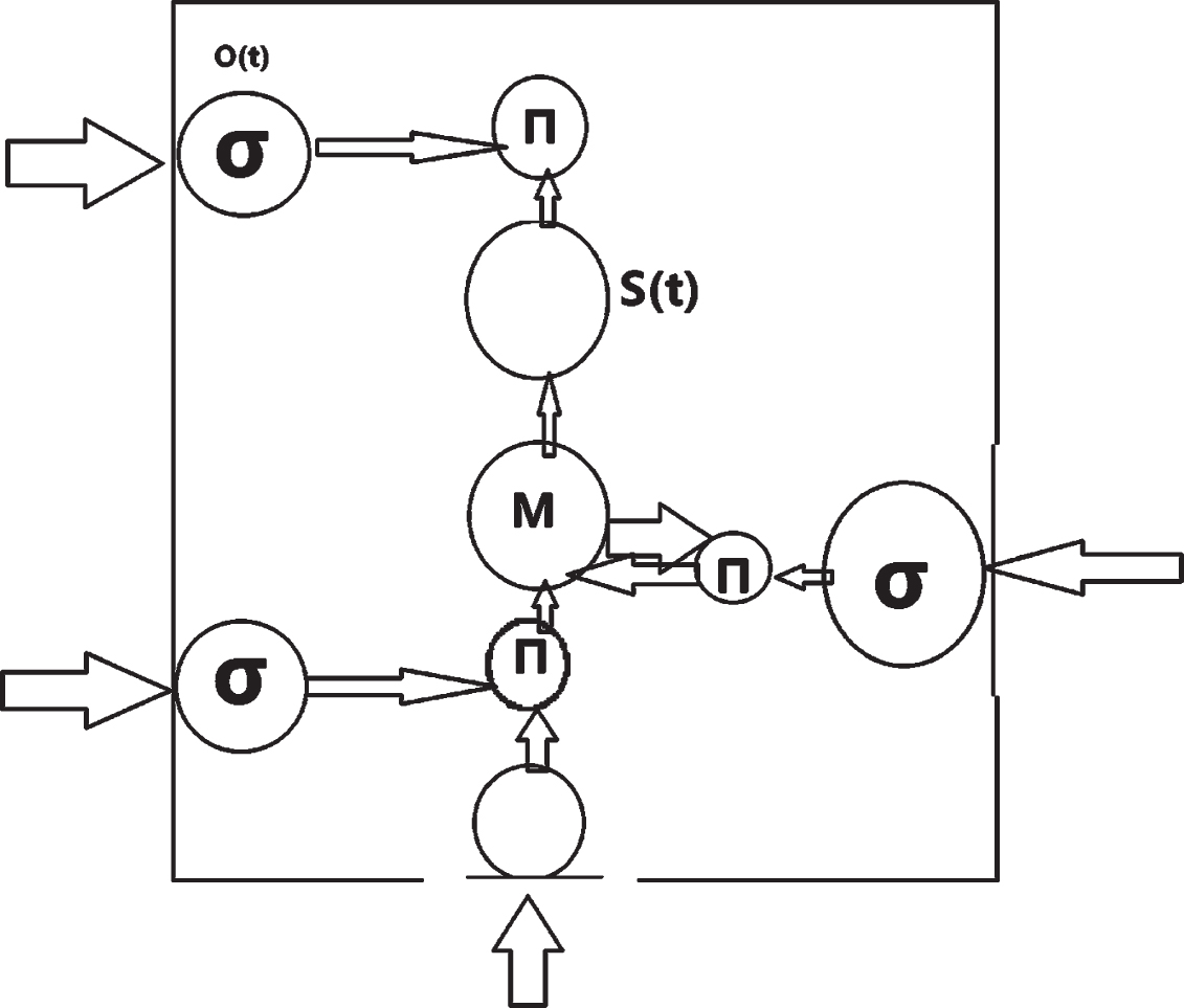
The network structure of LSTM is similar to that of ordinary recurrent NN, and it is also composed of three layers: input layer, hidden layer and output layer. The structure of the LSTM memory module is shown in Fig. 2. Through the control gate, LSTM can control the disturbance degree of new information to the saved information of neurons, so that LSTM model can save and transfer information for a long time. Among them, G (T), s (T) represent input and output elements respectively, m represent memory elements, I (T), O (T), f (T) represent input, output control gates and forgetting control gates respectively and their calculation methods. From Fig. 2, it can be seen that the three control gates have an impact on the memory of LSTM by connecting to the three multiplication units respectively, so as to control the reading, writing and forgetting operations of memory units. If the input length of the model is t and the input sequence is x, at time t, the state of the j-th memory module of the L-th layer can be expressed by the following formula:
Fig. 2
Structure diagram of LSTM memory module.
(16)
(17)
(18)
(19)
(20)
(21)
In the training process, the error back propagation algorithm is used to train the recurrent NN in this paper. The training objective function is to minimize the negative logarithm loss function as shown in Equation 22.
(22)
The loss function shows the classification performance of the algorithm. In each training, when l(T) does not change any more, the learning rate will be reduced appropriately. After the LSTM NN in this paper is trained, the test data will be used to test it.
4Experience and result
4.1LSTM NN test
The composition of the LSTM NN used in this case is shown in Fig. 3, which contains two hidden layers, each layer contains 200 LSTM memory modules. The input of the model is the eigenvector of an 8-D wind turbine bearing fault in Section 2. The output of the first hidden layer is the input of the second hidden layer. The output layer is composed of four softmax multi classification units, corresponding to a 4-bit fault code. The meaning of the output unit is shown in Table 1. They give the probability that the failure of wind turbine rolling bearing belongs to a certain class C at time t, and the calculation method is as follows:
Fig. 3
LSTM NN structure.
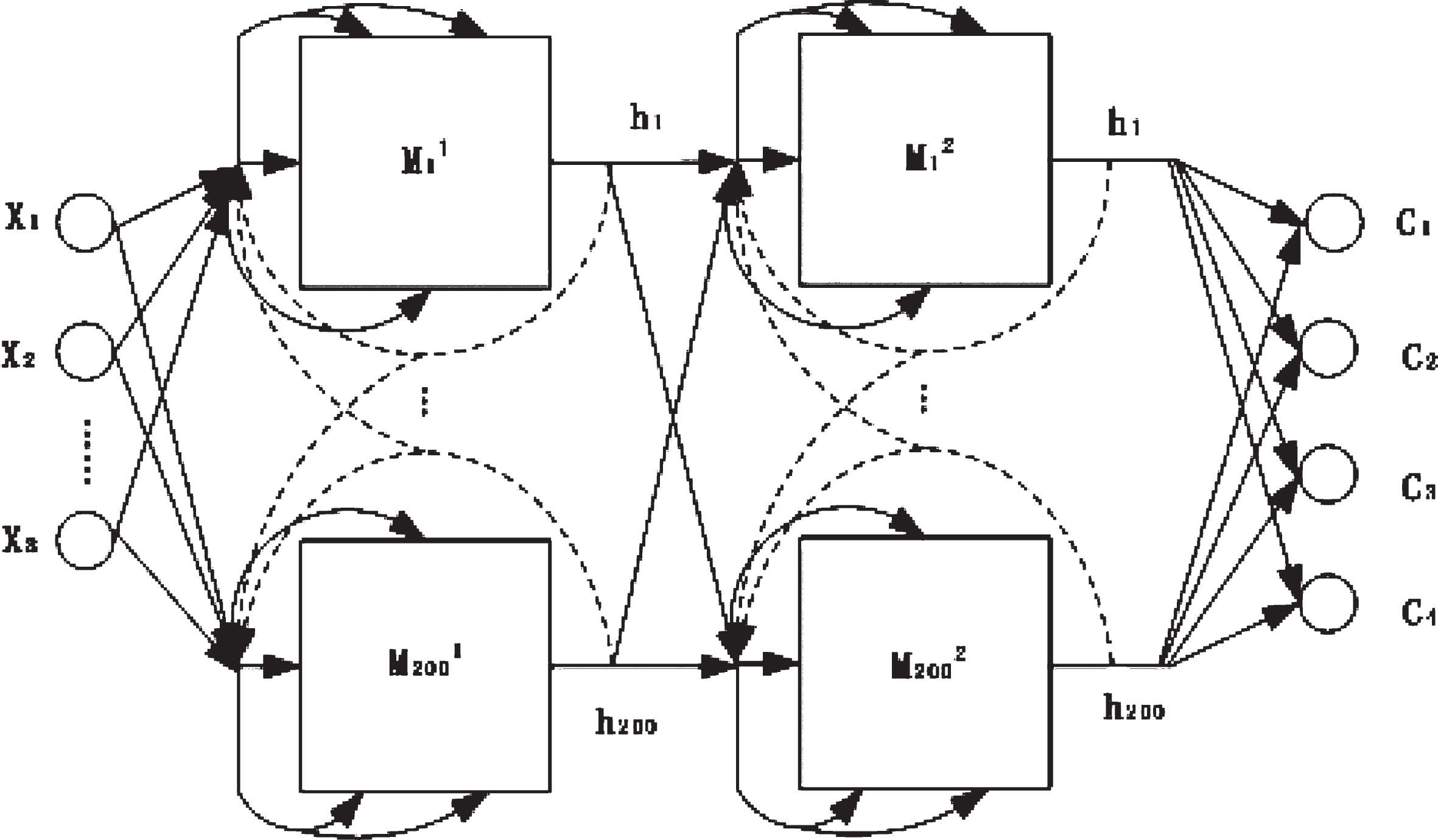
Table 1
Meaning of output unit
| Significance | Output unit C1 | Output unit C2 | Output unit C3 | Output unit C4 |
| Rolling body spalling | 1 | 0 | 0 | 0 |
| Inner ring peeling | 0 | 1 | 0 | 0 |
| Outer ring peeling | 0 | 0 | 1 | 0 |
| Normal | 0 | 0 | 0 | 1 |
(23)
In order to verify the effectiveness of this method, the rolling bearing vibration signals of 4 wind turbines of the same type in a wind farm in North China are selected as sample data, which can be divided into two parts: training data and test data. The energy characteristics of each frequency band are obtained to form the eigenvector of the sample. Among them, the length of training data is 24576, and the length of test data is 8192.
The trained LSTM NN is used to process four groups of data to be tested, and the fault diagnosis results are shown in Table 2.
Table 2
Diagnostic results
| Data value | Output results | Loss function value | Diagnostic results | Actual results | |||
| First set of test data | 0.996316 | 0.001471 | 0.001197 | 0.001003 | 4.7×10⁻⁶ | Rolling body spalling | Rolling body spalling |
| Second set of test data | 0.001949 | 0.995261 | 0.001558 | 0.001235 | 7.81×1;10–6 | Inner ring peeling | Inner ring peeling |
| Third set of test data | 0.001975 | 0.002176 | 0.994750 | 0.001335 | 9.8×1;10–6 | Outer ring peeling | Outer ring peeling |
| The fourth group of test data | 0.000809 | 0.001119 | 0.000923 | 0.997260 | 2.08×1;10–6 | Normal | Normal |
4.2PSO optimized NN algorithm
In particular, some wind farms in China are located in mountainous or hilly areas, and the airflow is distorted by the terrain, which makes the wind turbines work under complex alternating load for a long time. Due to the uncertainty of wind power, the speed of wind turbine is constantly changing. The internal structure of the gearbox is complex. Vibration signal usually has amplitude modulation and frequency modulation. These components are superimposed and coupled with each other, which makes the spatial distribution of the signal disordered. The characteristics make the analysis of wind turbine vibration signal more complex.
Information entropy is a measure of the overall average uncertainty of the whole signal source. The smaller the information entropy is, the more certain the information is, the less disordered the information is, and vice versa. The common information entropy includes power spectrum entropy, wavelet entropy and singular spectrum entropy.
When the gear fails, the vibration energy will change greatly. Kurtosis coefficient and skewness coefficient reflect the impact energy, which are the common indexes for gear fault diagnosis.
For nonlinear systems, the fractal dimension describes the dissipative energy of the system, which can reflect the irregularity and instability of vibration signals. The larger the fractal dimension is, the greater the dissipation energy is, and the smaller the fractal dimension is, the smaller the dissipation energy is. Fractal dimension includes correlation dimension, box dimension and energy dimension.
Considering the uncertainty, nonstationarity and complexity of wind turbine is selected as the eigenvalues of wind turbine gearbox fault diagnosis.
Taking 1.5 MW wind turbine of a wind farm as the research object, the vibration speed signal is collected. The sampling frequency is 5120 Hz, and there are 8192 sampling points. The data is denoised by wavelet transform. Some training samples are shown in Table 3.
Table 3
Training sample of eigenvalue for gearbox fault of wind turbinet
| Gear mode | Power spectral entropy | Wavelet entropy | Kurtosis | Skewness | Correlation dimension | Box dimension | Target vector |
| Normal state | 1.1958 | 0.9016 | 0.0906 | 1.6256 | 4.9068 | 1.5113 | 000 |
| Wear condition | 1.4296 | 0.7984 | –0.2827 | 1.4188 | 4.9117 | 1.5026 | 010 |
| Broken teeth state | 2.5655 | 1.8211 | 4.7560 | 2.1916 | 9.3745 | 1.5144 | 001 |
Since the three-layer BPNN with a hidden layer can complete any function mapping from n-dimension to m-dimension, a three-layer BP network structure is established in this paper.
According to the characteristic value and the number of fault types of gearbox, the number of input nodes, hidden layer nodes and output layer nodes of BPNN are 6, 13 and 3 respectively. Tansig is a tangent function of Singmoid type, and logsig is a logarithmic function of Sigmoid type. Trainlm is used as the training function. The training times of the network is 1000, the learning efficiency is 0.1, and the error of the training target is 0.001.
The acceleration constant C1 = C2 = 2, and the maximum speed vmax = 1.
The inertia weight W in the speed update formula of PSO determines the influence degree of particle’s previous velocity on the current velocity, so as to balance the data fusion in the two algorithms. The inertia weight adjustment formula is as follows:
(23)
Where, I –the current iteration; Imax –the maximum number of iterations. The maximum value of inertia weight wmax = 1, the minimum value wmin = 0.2.
After the establishment and training of the network, test the network. Some test samples are shown in Table 4.
Table 4
Wind turbine gearbox fault eigenvalue test sample
| Gear mode | Power spectral entropy | Wavelet entropy | Kurtosis | Skewness | Correlation dimension | Box dimension |
| Normal state | 0.9531 | 0.6396 | –0.3855 | 1.5126 | 4.8237 | 1.4663 |
| Wear condition | 1.4396 | 1.2948 | –0.7156 | 1.4132 | 5.5511 | 1.4936 |
| Broken teeth state | 2.2020 | 1.9137 | 2.4511 | 2.0148 | 8.9638 | 1.5128 |
After three groups of test data are processed by trained NN, the first group of data can be judged as normal state, the second group of data as worn state, and the third group of data as broken teeth state. Some output fault diagnosis results are shown in Table 5. Therefore, the PSO combined with NN algorithm are used.
Table 5
State identification results
| Gear mode | Number | Y1 | Y2 | Y3 |
| Normal state | 1 | 0.0000 | 0.0258 | 0.0147 |
| Wear condition | 2 | 0.0168 | 0.9369 | 0.0000 |
| Broken teeth state | 3 | 0.0000 | 0.0000 | 1.1000 |
5Conclusions
In this paper, PSO algorithm is used to combine PSO with BPNN. PSO algorithm has good global search ability, can optimize the weight and deviation of BP network, reduce the risk of BPNN algorithm falling into local optimal solution, improve the training efficiency of NN and accelerate the convergence speed of network. Wavelet packet transform is used to process the vibration data of wind turbine rolling bearing, and the fault characteristics of wind turbine rolling bearing are effectively extracted. A fault diagnosis model of wind turbine rolling bearing based on wavelet packet transform and long-term memory NN is established. By inputting the fault feature vector extracted from wavelet packet transform into long and short time memory NN, the accurate diagnosis of three kinds of multi faults of wind turbine rolling bearing is realized. Through the analysis of an example, it is verified that the diagnosis results of this method are consistent with the actual fault diagnosis results of wind turbine rolling bearing, and the diagnosis accuracy is high, which shows the effectiveness of the method. The operation condition of wind turbine is complex. With the large-scale wind turbine, its structure is more and more complex. Therefore, the effective maintenance of wind turbine becomes more and more important. This method brings great changes to the intelligent fault diagnosis of wind turbine drive shaft system.
Acknowledgments
This paper is supported by the International Co-operation Tackling of Key Scientific and Technical Problems Project of the Science Department of Henan Province. (No. 162102410080).
References
[1] | Ren C. , An N. , Wang J. , et al., Optimal parameters selection for BP neural network based on particle swarm optimization: A case study of wind speed forecasting, Knowledge Based Systems 56: (jan.) ((2014) ), 226–239. |
[2] | Zhang K. , Qu Z. , Dong Y. , et al., Research on a combined model based on linear and nonlinear features - A case study of wind speed forecasting, Renewable Energy 130: (JAN.) ((2019) ), 814–830. |
[3] | Das S.S. , Das Sharma K. , Chandra J.K. , et al., Secure image transmission based on visual cryptography scheme and artificial neural network-particle swarm optimization-guided adaptive vector quantization, Journal of Electronic Imaging 28: (3) ((2019) ), 31.1–31.11. |
[4] | Zhu C. , Zhang J. , Liu Y. , et al., Comparison of GA-BP and PSO-BP neural network models with initial BP model for rainfall-induced landslides risk assessment in regional scale: a case study in Sichuan, China, Natural Hazards 2020: , 1–32. |
[5] | Ling Q.H. , Song Y.Q. , Han F. , et al., An improved learning algorithm for random neural networks based on particle swarm optimization and input-to-output sensitivity, Cognitive Systems Research 53: (JAN.) ((2019) ), 51–60. |
[6] | Mhamdi B. , Microwave imaging based on two hybrid particle swarm optimization approaches, International Journal of Microwave and Wireless Technologies 11: (3) ((2019) ), 268–275. |
[7] | Pan L. , Node localization method for massive sensor networks based on clustering particle swarm optimization in cloud computing environment, International Journal of Wavelets Multiresolution and Information Processing 18: (9) ((2019) ). |
[8] | Luo X. , Yang B. and Qian H.J. , Adaptive Synthesis for Resonator-Coupled Filters Based on Particle Swarm Optimization, IEEE Transactions on Microwave Theory and Techniques 67: (2) ((2019) ), 712–725. |
[9] | Chang E.C. , Cheng C.A. and Yang L.S. , Nonsingular Terminal Sliding Mode Control Based on Binary Particle Swarm Optimization for DC–AC Converters, Energies 12: (11) ((2019) ), 2099. |
[10] | Xing H.H. , et al., Risk assessment of earthquake network public opinion based on global search BP neural network, Plos One (2019). |
[11] | Xu Y.X. , Niu L.C. , Yang H. , et al., Optimization of Lithium Battery Pole Piece Thickness Control System Based on GA-BP Neural Network, Journal of Nanoelectronics and Optoelectronics (2019), 880–886. |
[12] | No-reference image quality assessment based on AdaBoost_BP neural network in wavelet domain, Journal of Systems Engineering and Electronics 30: (02) ((2019) ), 5–19. |
[13] | Malik K. , Optimal Travel Route Recommendation Mechanism Based on Neural Networks and Particle Swarm Optimization for Efficient Tourism Using Tourist Vehicular Data, Sustainability 11: (12) ((2019) ), 3357. |
[14] | Yang L. , Wang F. , Zhang J. , et al., Remaining useful life prediction of ultrasonic motor based on Elman neural network with improved particle swarm optimization, Measurement (2019), 123–129. |
[15] | Yang L. and Chen H. , Fault diagnosis of gearbox based on RBF-PF and particle swarm optimization wavelet neural network, Neural Computing & Applications 31: (9) ((2019) ), 4463–4478. |
[16] | He H. and Zhang X. , A Variable In ate Firing Optimization of Launcher Based on Particle Swarm Optimization, Propellants Explosives Pyrotechnics 44: (5) ((2019) ). |
[17] | Su T.J. , Chen Y.F. and Lo K.L. , Design chip position of printed circuit board based on particle swarm optimization, Modern Physics Letters B 33: (14n15) ((2019) ), 1940043. |
[18] | El Hazzat S. , Merras M. , El Akkad N. , et al., Enhancement of sparse 3D reconstruction using a modified match propagation based on particle swarm optimization, Multimedia Tools and Applications 78: (11) ((2019) ), 14251–14276. |
[19] | Yanpeng Z. , Hybrid kernel extreme learning machine for evaluation of athletes’ competitive ability based on particle swarm optimization, Computers & Electrical Engineering 73: ((2019) ), 23–31. |
[20] | Zhen X. , Enze Z. and Qingwei C. , Rotary unmanned aerial vehicles path planning in rough terrain based on multi-objective particle swarm optimization, Journal of Systems Engineering and Electronics 31: (1) ((2020) ), 130–141. |


