
Overfitting, robustness, and malicious algorithms: A study of potential causes of privacy risk in machine learning
Abstract
Machine learning algorithms, when applied to sensitive data, pose a distinct threat to privacy. A growing body of prior work demonstrates that models produced by these algorithms may leak specific private information in the training data to an attacker, either through the models’ structure or their observable behavior. This article examines the factors that can allow a training set membership inference attacker or an attribute inference attacker to learn such information. Using both formal and empirical analyses, we illustrate a clear relationship between these factors and the privacy risk that arises in several popular machine learning algorithms.
We find that overfitting is sufficient to allow an attacker to perform membership inference and, when the target attribute meets certain conditions about its influence, attribute inference attacks. We also explore the connection between membership inference and attribute inference, showing that there are deep connections between the two that lead to effective new attacks. We show that overfitting is not necessary for these attacks, demonstrating that other factors, such as robustness to norm-bounded input perturbations and malicious training algorithms, can also significantly increase the privacy risk. Notably, as robustness is intended to be a defense against attacks on the integrity of model predictions, these results suggest it may be difficult in some cases to simultaneously defend against privacy and integrity attacks.
1.Introduction
Machine learning has emerged as an important technology, enabling a wide range of applications including computer vision, machine translation, health analytics, and advertising, among others. The fact that many compelling applications of this technology involve the collection and processing of sensitive personal data has given rise to concerns about privacy [3,9,14,22,23,39,54,66,67]. In particular, when machine learning algorithms are applied to private training data, the resulting models might unwittingly leak information about that data through either their behavior (i.e., black-box attack) or the details of their structure (i.e., white-box attack).
Although there has been a significant amount of work aimed at developing machine learning algorithms that satisfy definitions such as differential privacy [18,19,38,60,67,71], the factors that bring about specific types of privacy risk in applications of standard machine learning algorithms are not well understood. Following the connection between differential privacy and stability from statistical learning theory [5,11,18,19,60,63], one such factor that has started to emerge [23,54] as a likely culprit is overfitting. A machine learning model is said to overfit to its training data when its performance on unseen test data diverges from the performance observed during training, i.e., its generalization error is large. The relationship between privacy risk and overfitting is further supported by recent results that suggest the contrapositive, i.e., under certain reasonable assumptions, differential privacy [19] and related notions of privacy [4,64] imply good generalization. However, a precise account of the connection between overfitting and the risk posed by different types of attack remains unknown.
In this article, we characterize the effect that overfitting has on the advantage of adversaries who attempt to infer specific facts about the data used to train machine learning models. We formalize quantitative advantage measures that capture the privacy risk to training data posed by two types of attack, namely membership inference [39,54] and attribute inference [22,23,66,67]. For each type of attack, we analyze the advantage in terms of generalization error (overfitting) for several concrete black-box adversaries. While our analysis necessarily makes formal assumptions about the learning setting, we show that our analytic results hold on several real-world datasets by controlling for overfitting through regularization and model structure.
In addition, we explore other factors that can also aid the attacker. Previously, it has been shown that, for Boolean functions, the Boolean influence [44,66], which measures the extent to which a particular input to a function can cause changes to its output, is also relevant to privacy risk. Our analysis in the regression setting is consistent with this result, showing that the influence of the target attribute is also a key factor that determines the effectiveness of attribute inference. Furthermore, we demonstrate that privacy risk can arise even when the model does not overfit, and surprisingly, that black-box adversaries can recover substantial information about the training data. To illustrate this point, we show how to construct a malicious training algorithm that colludes with an attacker to surreptitiously leak information about the training data, while imposing minimal changes on the model’s normal behavior.
Finally, we identify robustness to norm-bounded input perturbations, which has been proposed as a defense against attacks on the integrity of model predictions [40,65], as a possible vulnerability against privacy attacks. In particular, we show that when robustness is achieved through adversarial training [40], there exist membership adversaries with significantly greater advantage than when training a corresponding model using conventional methods. This analysis of robust models is a major addition to the conference version [68] of this article.
1.1.Membership inference
Training data membership inference attacks aim to determine whether a given data point was present in the training data used to build a model. Although this may not at first seem to pose a serious privacy risk, the threat is clear in settings such as health analytics where the distinction between case and control groups could reveal an individual’s sensitive conditions. This type of attack has been extensively studied in the adjacent area of genomics [28,50], and more recently in the context of machine learning [39,54].
Our analysis shows a clear dependence of membership advantage on generalization error (Section 3.2), and in some cases the relationship is directly proportional (Theorem 2). Our experiments on real data confirm that this connection matters in practice (Section 7.2), even for models that do not conform to the formal assumptions of our analysis. In one set of experiments, we apply a particularly straightforward attack to deep convolutional neural networks (CNNs) using several datasets examined in prior work on membership inference. Despite requiring significantly less computation and adversarial background knowledge, our attack performs almost as well as a recently published attack [54].
Our results illustrate that overfitting is a sufficient condition for membership vulnerability in popular machine learning algorithms. However, it is not a necessary condition (Theorem 4). In fact, under certain assumptions that are commonly satisfied in practice, we show that a stable training algorithm (i.e., one that does not overfit) can be subverted so that the resulting model is nearly as stable but reveals exact membership information through its black-box behavior. This attack is suggestive of algorithm substitution attacks from cryptography [7] and makes adversarial assumptions similar to those of other recent privacy attacks [57]. We implement this construction to train deep CNNs (Section 7.4) and observe that, regardless of the model’s generalization behavior, the attacker can recover membership information while incurring very little penalty to predictive accuracy.
1.2.Attribute inference
In an attribute inference attack, the adversary uses a machine learning model and incomplete information about a data point to infer the missing information for that point. For example, in work by Fredrikson et al. [23], the adversary is given partial information about an individual’s medical record and attempts to infer the individual’s genotype by using a model trained on similar medical records.
We formally characterize the advantage of an attribute inference adversary as its ability to infer a target feature given an incomplete point from the training data, relative to its ability to do so for points from the general population (Section 4). This approach is distinct from the way that attribute advantage has largely been characterized in prior work [22,23,66], which prioritized empirically measuring advantage relative to a simulator who is not given access to the model. We offer an alternative definition of attribute advantage (Definition 6) that corresponds to this characterization and argue that it does not isolate the risk that the model poses specifically to individuals in the training data.
Our formal analysis shows that attribute inference, like membership inference, is indeed sensitive to overfitting. However, we find that influence must be factored in as well to understand when overfitting will lead to privacy risk (Section 4.1). Interestingly, the risk to individuals in the training data is greatest when these two factors are “in balance”. Regardless of how large the generalization error becomes, the attacker’s ability to learn more about the training data than the general population vanishes as influence increases.
1.3.Connection between membership and attribute inference
The two types of attack that we examine are deeply related. We build reductions between the two by assuming oracle access to either type of adversary. Then, we characterize each reduction’s advantage in terms of the oracle’s assumed advantage. Our results suggest that attribute inference may be “harder” than membership inference: attribute advantage implies membership advantage (Theorem 6), but there is currently no similar result in the opposite direction.
Our reductions are not merely of theoretical interest. Rather, they function as practical attacks as well. We implemented a reduction for attribute inference and evaluated it on real data (Section 7.3). Our results show that when generalization error is high, the reduction adversary can outperform an attribute inference attack given in [23] by a significant margin.
1.4.Membership inference on robust models
Beyond privacy, another well-known type of attack in the context of machine learning seeks to induce errant predictions from the model. Prior work on these attacks [26,46,47,59] has shown that it is often possible to make small, visually imperceptible changes to image features such that a deep convolutional neural network (CNN) classifier is “tricked” into labeling the resulting image as something completely different from the true label, and in many cases to do so arbitrarily at the attacker’s discretion. This has motivated a growing body of subsequent work on methods for training robust models [13,40,65], especially for the case of CNNs, which resist these attacks by remaining insensitive to norm-bounded input perturbations.
Intuitively, robust training methods produce models with decision boundaries that are located suitably far from each of the training points. If the distances between decision boundaries and training points are often minimal, and the model fits the training points closely in at least one direction, then the model will be less likely to make comparably robust predictions on test points. We observe that an attacker might be able to evaluate the model’s level of robustness on a given input to draw inferences about membership.
Building from this intuition, we argue both analytically and experimentally that robustness can be another source of membership advantage. Applying a general result (Theorem 2) that leverages classification error for membership inference, we show that an adversary can use a model’s robust generalization error, which is a measure of overfitting that takes robustness into account, to gain membership advantage (Section 6). Our experimental results show that when adversarial training with projected gradient descent [40] is used to achieve robustness, the robust generalization error is often greater than the standard generalization error (Section 7.5), thus indicating that attacks on robust models can be more effective than those based on overfitting alone. We then present an attack that operationalizes the above intuition in greater detail by estimating the distance to the nearest decision boundary, and show experimentally that this can leak significantly more information than the robust generalization error alone. In particular, this attack predicts membership with up to 90% accuracy on a benchmark image classification dataset.
These results suggest that in some cases, robustness and training set privacy may conflict with each other, so that resistance to one type of attack may make a model more vulnerable to a different type of attack. Finding a way to resolve this tension is an important direction for future work.
1.5.Summary
This article explores the factors that contribute to privacy risk in machine learning models. We present new formalizations of membership inference attacks (Section 3) and attribute inference attacks (Section 4), which allow us to analyze the privacy risk that black-box variants of these attacks pose to individuals in the training data. We give analytic quantities for the attacker’s performance in terms of generalization error and influence and conclude that certain configurations imply privacy risk. We then study the underlying connections between membership and attribute inference attacks (Section 5), finding surprising relationships that give insight into the relative difficulty of the attacks and lead to new attacks that work well on real data. We also show that overfitting is not the only source of privacy risk by constructing adversaries that leverage a malicious training algorithm (Section 3.4) or robustness (Section 6) to infer membership information. Finally, we present our empirical results (Section 7), which mostly align with the analytical results in Sections 3–6 and show that our attacks are effective on real-world datasets.
2.Background
Throughout the article we focus on privacy risks related to machine learning algorithms. We begin by introducing basic notation and concepts from learning theory.
2.1.Notation and preliminaries
Let
Unless stated otherwise, our results pertain to the standard machine learning setting, wherein a model
2.2.Stability and generalization
An algorithm is stable if a small change to its input causes limited change in its output. In the context of machine learning, the algorithm in question is typically a training algorithm A, and the “small change” corresponds to the replacement of a single data point in S. This is made precise in Definition 1.
Definition 1
Definition 1(On-Average-Replace-One (ARO) Stability).
Given
Stability is closely related to the popular notion of differential privacy [17] given in Definition 2.
Definition 2
Definition 2(Differential privacy).
An algorithm
When a learning algorithm is not stable, the models that it produces might overfit to the training data. Overfitting is characterized by large generalization error, which is defined below.
Definition 3
Definition 3(Average generalization error).
The average generalization error of a machine learning algorithm A on
In other words,
It is important to note that Definition 3 describes the average generalization error over all training sets, as contrasted with another common definition of generalization error
3.Membership inference attacks
In a membership inference attack, the adversary attempts to infer whether a specific point was included in the dataset used to train a given model. The adversary is given a data point
Experiment 1 below formalizes membership inference attacks. The experiment first samples a fresh dataset from
Experiment 1
Experiment 1(Membership experiment Exp M ( A , A , n , D )
Let
(1) Sample
(2) Choose
(3) Draw
(4)
Definition 4
Definition 4(Membership advantage).
The membership advantage of
Equivalently, the right-hand side can be expressed as the difference between
Using Experiment 1, Definition 4 gives an advantage measure that characterizes how well an adversary can distinguish between
In fact, the only way to gain advantage is through access to the model. In the membership experiment
3.1.Bounds from differential privacy
Our first result (Theorem 1) bounds the advantage of an adversary who attempts a membership attack on a differentially private model [17]. Differential privacy imposes strict limits on the degree to which any point in the training data can affect the outcome of a computation, and it is commonly understood that differential privacy will limit membership inference attacks. Thus it is not surprising that the advantage is limited by a function of ϵ.
Theorem 1.
Let A be an ϵ-differentially private learning algorithm and
Proof.
Given
Without loss of generality for the case where models reside in an infinite domain, assume that the models produced by A come from the set
Wu et al. [67, Section 3.2] present an algorithm that is differentially private as long as the loss function ℓ is strongly convex and Lipschitz. Moreover, they prove that the performance of the resulting model is close to the optimal. Combined with Theorem 1, this provides us with a bound on membership advantage when the loss function is strongly convex and Lipschitz.
However, this and other methods of achieving differential privacy, and by extension a bound on membership advantage, may decrease the utility of the resulting model. In particular, Theorem 1 does not give us a meaningful bound unless
3.2.Membership attacks and generalization
In this section, we consider several membership attacks that make few, common assumptions about the model
For each attack, we express the advantage of the attacker as a function of the extent of the overfitting, thereby showing that the generalization behavior of the model is a strong predictor for vulnerability to membership inference attacks. In Section 7.2, we demonstrate that these relationships often hold in practice on real data, even when the assumptions used in our analysis do not hold.
Bounded loss function. We begin with a straightforward attack that makes only one simple assumption: the loss function is bounded by some constant B. Then, with probability proportional to the model’s loss at the query point z, the adversary predicts that z is not in the training set. The attack is formalized in Adversary 1.
Adversary 1
Adversary 1(Bounded loss function).
Suppose
(1) Query the model to get
(2) Output 1 with probability
Theorem 2 states that the membership advantage of this approach is proportional to the generalization error of A, showing that advantage and generalization error are closely related in many common learning settings. In particular, classification settings, where the 0–1 loss function is commonly used,
Theorem 2.
The advantage of Adversary 1 is
Proof.
The proof is as follows:
Gaussian error. Whenever the adversary knows the exact error distribution, it can simply compute which value of b is more likely given the error of the model on z. This adversary is described formally in Adversary 2. While it may seem far-fetched to assume that the adversary knows the exact error distribution, linear regression models implicitly assume that the error of the model is normally distributed. In addition, the standard errors
Adversary 2
Adversary 2(Threshold).
Suppose
(1) Query the model to get
(2) Let
In regression problems that use squared-error loss, the magnitude of the generalization error depends on the scale of the response y. For this reason, in the following we use the ratio
Theorem 3.
Suppose
Proof.
We have
3.3.Unknown standard error
In practice, models are often published with just one value of standard error, so the adversary often does not know how
Alternatively, if the adversary knows which machine learning algorithm was used, it can repeatedly sample
3.4.Malicious training algorithm
The results in the preceding sections show that overfitting is sufficient for membership advantage. However, models can leak information about the training set in other ways, and thus overfitting is not necessary for membership advantage. For example, the learning algorithm can produce models that simply output a lossless encoding of the training dataset. This example may seem unconvincing for several reasons: the leakage is obvious, and the “encoded” dataset may not function well as a model. In the rest of this section, we present a pair of colluding training algorithm and adversary that does not have the above issues but still allows the attacker to learn the training set almost perfectly. This is in the framework of an algorithm substitution attack (ASA) [7], where the target algorithm, which is implemented by closed-source software, is subverted to allow a colluding adversary to violate the privacy of the users of the algorithm. All the while, this subversion remains impossible to detect. Algorithm 1 and Adversary 3 represent a similar security threat for learning algorithms with bounded loss function. While the attack presented here is not impossible to detect, on points drawn from
The main result is given in Theorem 4, which shows that any ARO-stable learning algorithm A, with a bounded loss function operating on a finite domain, can be modified into a vulnerable learning algorithm
Theorem 4.
Let
The proof of Theorem 4 involves constructing a learning algorithm
Algorithm 1
Algorithm 1(Colluding training algorithm A C
Let
(1) Supplement S using
(2) Return
Adversary 3
Adversary 3(Colluding adversary A C
Let
(1) For
(2) Output 0 if
Algorithm 1 will not work well in practice for many classes of models, as they may not have the capacity to store the membership information needed by the adversary while maintaining the ability to generalize. Interestingly, in Section 7.4 we empirically demonstrate that deep convolutional neural networks (CNNs) do in fact have this capacity and generalize perfectly well when trained in the manner of
Before we give the formal proof, we note a key difference between Algorithm 1 and the construction used in the proof. Whereas the model returned by Algorithm 1 belongs to the same class as those produced by A, in the formal proof the training algorithm can return an arbitrary model as long as its black-box behavior is suitable.
Proof.
The proof constructs a learning algorithm and adversary who share a set of k keys to a pseudorandom function. The secrecy of the shared key is unnecessary, as the proof only relies on the uniformity of the keys and the pseudorandom functions’ outputs. The primary concern is with using the pseudorandom function in a way that preserves the stability of A as much as possible.
Without loss of generality, assume that
Now observe that A is ARO-stable with rate
The formal study of ASAs was introduced by Bellare et al. [7], who considered attacks against symmetric encryption. Subsequently, attacks against other cryptographic primitives were studied as well [2,6,24]. The recent work of Song et al. [57] considers a similar setting, wherein a malicious machine learning provider supplies a closed-source training algorithm to users with private data. When the provider gets access to the resulting model, it can exploit the trapdoors introduced in the model to get information about the private training dataset. However, to the best of our knowledge, a formal treatment of ASAs against machine learning algorithms has not been given yet. We leave this line of research as future work, with Theorem 4 as a starting point.
4.Attribute inference attacks
We now consider attribute inference attacks, where the goal of the adversary is to guess the value of the sensitive features of a data point given only some public knowledge about it and the model. To make this explicit in our notation, in this section we assume that data points are triples
Attribute inference is formalized in Experiment 2, which proceeds much like Experiment 1. An important difference is that the adversary is only given partial information
Experiment 2
Experiment 2(Attribute experiment Exp A ( A , A , n , D )
Let
(1) Sample
(2) Choose
(3) Draw
(4)
In the corresponding advantage measure shown in Definition 5, our goal is to measure the amount of information about the target
Definition 5
Definition 5(Attribute advantage).
The attribute advantage of
The attribute advantage can also be expressed as
This definition has the side effect of incentivizing the adversary to “game the system” by performing poorly when it thinks that
Definition 6
Definition 6(Alternative attribute advantage).
Let
Definitions 5 and 6 measure the privacy risk of two fundamentally different types of actions. Broadly, there are two ways for a model to perform better on the training data: it can overfit to the training data, or it can learn a general trend in the distribution
In this article, we analyze the privacy risk that the model poses to the members of the training set in particular. We thereby explore the implications of the view that, if the model learns a general trend in the distribution
4.1.Inversion, generalization, and influence
The case where φ simply removes the sensitive attribute t from the data point
In this section, we look at the model inversion attack of Fredrikson et al. [23] under the advantage given in Definition 5. We point out that this is a novel analysis, as this advantage is defined to reflect the extent to which an attribute inference attack reveals information about individuals in S. While prior work [22,23] has empirically evaluated attribute accuracy over corresponding training and test sets, our goal is to analyze the factors that lead to increased privacy risk specifically for members of the training data. To that end, we illustrate the relationship between advantage and generalization error as we did in the case of membership inference (Section 3.2). We also explore the role of feature influence, which in this case corresponds to the degree to which changes to a sensitive feature of x affects the value
The attack described by Fredrikson et al. [23] is intended for linear regression models and is thus subject to the Gaussian error assumption discussed in Section 3.2. In general, when the adversary can approximate the error distribution reasonably well, e.g., by assuming a Gaussian distribution whose standard deviation equals the published standard error value, it can gain advantage by trying all possible values of the sensitive attribute. We denote the adversary’s approximation of the error distribution by
Adversary 4
Adversary 4(General).
Let
(1) Query the model to get
(2) Let
(3) Return the result of
When analyzing Adversary 4, we are clearly interested in the effect that generalization error will have on advantage. Given the results of Section 3.2, we can reasonably expect that large generalization error will lead to greater advantage. However, as pointed out by Wu et al. [66], the functional relationship between t and
The attack considered here applies to linear regression models, and Boolean influence is not suitable for use in this setting. However, an analogous notion of influence that characterizes the magnitude of change to
Binary variable with uniform prior. The first part of our analysis deals with the simplest case where
Theorem 5.
Let t be drawn uniformly from
Proof.
Given the assumptions made in this setting, we can describe the behavior of
Clearly, the advantage will be zero when there is no generalization error (
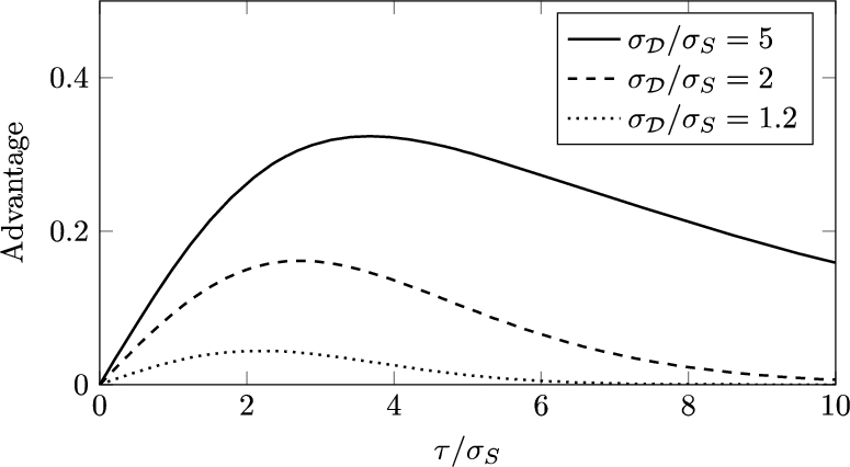
Figure 1 shows the effect of changing τ as the ratio
Fig. 1.
The advantage of Adversary 4 as a function of t’s influence τ. Here t is a uniformly distributed binary variable.
General case. Sometimes the uniform prior for t may not be realistic. For example, t may represent whether a patient has a rare disease. In this case, we weight the values of
Clearly
In general, the advantage can be computed using Equation (5). We first figure out when the adversary outputs
5.Connection between membership and attribute inference
In this section, we examine the underlying connections between membership and attribute inference attacks. Our approach is based on reduction adversaries that have oracle access to one type of attack and attempt to perform the other type of attack. We characterize the advantage of each reduction adversary in terms of the advantage of its oracle. In Section 7.3, we implement the most sophisticated of the reduction adversaries described here and show that on real data it performs remarkably well, often outperforming Attribute Adversary 4 by large margins. We note that these reductions are specific to our choice of attribute advantage given in Definition 5. Analyzing the connections between membership and attribute inference using the alternative Definition 6 is an interesting direction for future work.
5.1.From membership to attribute
We start with an adversary
Adversary 5
Adversary 5(Membership → attribute).
The reduction adversary
(1) Query the oracle to get
(2) Output 0 if
Theorem 6 shows that the membership advantage of this reduction exactly corresponds to the attribute advantage of its oracle. In other words, the ability to effectively infer attributes of individuals in the training set implies the ability to infer membership in the training set as well. This suggests that attribute inference is at least as difficult as than membership inference.
Theorem 6.
Let
Proof.
The proof follows directly from the definitions of membership and attribute advantages.
5.2.From attribute to membership
We now consider reductions in the other direction, wherein the adversary is given
Adversary 6
Adversary 6(Uniform attribute → membership).
Suppose that
(1) Choose
(2) Let
(3) Query
(4) If
The uniform choice of
In the computation of the advantage, we only consider the case where
Theorem 7 shows that the attribute advantage of
Theorem 7.
Let
Proof.
We first give an informal argument. In order for
Now we give the formal proof. Let
Adversary 6 has the obvious weakness that it can only return correct answers when it guesses the value of t correctly. Adversary 7 attempts to improve on this by making multiple queries to
Adversary 7
Adversary 7(Multi-query attribute → membership).
Suppose that
(1) Let
(2) For all
(3) Query
(4) Output
We evaluate this adversary experimentally in Section 7.3.
6.Membership inference on robust models
Beyond privacy, another well-studied type of attack on machine learning models targets the integrity of their predictions. In this context, an integrity attack seeks to induce errant predictions from the model by changing the model’s inputs in ways that are visually imperceptible, in the case of image models, or otherwise difficult for humans to detect [26,47]. Formally, given a point x and a desired prediction
In response to these findings, researchers have proposed robust learning algorithms that are resistant to these attacks. While the literature on robust statistics and learning predates interest in the attacks described above, the most recent work in this area [13,40,65] seeks methods that produce deep neural networks whose predictions remain consistent in quantifiable bounded regions around training and test points. In this section, we present membership adversaries that leverage this property to infer membership in the training set. In Section 7.5, we experimentally evaluate these attacks on models trained with a robust objective, and find that it is often possible to infer membership with significantly greater advantage than on models trained using conventional, non-robust methods. This suggests a potential tension between the integrity of models’ predictions and the confidentiality of their training data when certain robust learning methods are used.
Because most prior work in robust machine learning only consider the classification setting, we also limit ourselves to classification. In this setting, a natural loss function is the 0–1 loss, and Theorem 2 shows that our bounded-loss adversary (Adversary 1) achieves a membership advantage equal to the generalization error. However, for robust models the robustness is another source of membership information, and we show here how membership adversaries can use this information. In Section 7.5, we empirically verify that these adversaries can in some cases attain a higher membership advantage than the generalization error.
We first introduce a formal definition of robustness.
Definition 7
Definition 7(Robust loss).
Let d be a distance metric, ρ be a robustness parameter, and
We then define the robust generalization error, which is simply the generalization error (Definition 3) with the loss ℓ replaced by the robust loss
Definition 8
Definition 8(Robust generalization error).
The robust generalization error of a machine learning algorithm A on
Suppose ℓ is the 0–1 loss, as is often the case in classification models. Then, we say that a model is robust at the point
Adversary 8
Adversary 8(Robust classification).
Suppose
(1) Find a perturbed input
(2) Query the model to get
(3) Output
Ideally, we want the adversary to output the value of the robust loss
Theorem 8.
If the attack used by Adversary 8 always returns an
Proof.
The proof is as follows:
We now present a second membership adversary that leverages robustness. This adversary is a modification of the threshold adversary (Adversary 2). The threshold adversary is defined for the regression setting and bases its decisions on how far the prediction of the model is from the true value. By contrast, Adversary 9 is defined for the classification setting and bases its decisions on how far the decision boundary is from the given point.
Adversary 9
Adversary 9(Robust threshold).
For model
(1) Query the model, possibly multiple times, to find the value of
(2) Output
Although there is no general efficient method for determining the exact value of
To characterize the advantage of Adversary 9, we must make assumptions about the conditional distributions of
Instead, in this work we empirically evaluate this adversary by using an existing integrity attack to approximate
7.Evaluation
In this section, we evaluate the performance of the adversaries discussed in Sections 3, 4, 5, and 6. We compare the performance of these adversaries on real datasets with the analysis from previous sections and show that overfitting predicts privacy risk in practice as our analysis suggests. Our experiments use linear regression, tree, and deep convolutional neural network (CNN) models.
7.1.Methodology
7.1.1.Linear and tree models
We used the Python scikit-learn [48] library to calculate the empirical error
Eyedata. | This is gene expression data from rat eye tissues [51], as presented in the “flare” package of the R programming language. The inputs and the outputs are respectively stored in R as a |
IWPC. | This is data collected by the International Warfarin Pharmacogenetics Consortium [30] about patients who were prescribed warfarin. After we removed rows with missing values, 4819 patients remained in the dataset. The inputs to the model are demographic (age, height, weight, race), medical (use of amiodarone, use of enzyme inducer), and genetic (VKORC1, CYP2C9) attributes. Age, height, and weight are real-valued and were scaled to zero mean and unit variance. The medical attributes take binary values, and the remaining attributes were one-hot encoded. The output is the weekly dose of warfarin in milligrams. However, because the distribution of warfarin dose is skewed, IWPC concludes in [30] that solving for the square root of the dose results in a more predictive linear model. We followed this recommendation and scaled the square root of the dose to zero mean and unit variance. |
Netflix. | We use the dataset from the Netflix Prize contest [42]. This is a sparse dataset that indicates when and how a user rated a movie. For the output attribute, we used the rating of Dragon Ball Z: Trunks Saga, which had one of the most polarized rating distributions. There are 2416 users who rated this, and the ratings were scaled to zero mean and unit variance. The input attributes are binary variables indicating whether or not a user rated each of the other 17,769 movies in the dataset. |
7.1.2.Deep convolutional neural networks
We evaluated the membership inference attack on deep CNNs. In addition, we implemented the colluding training algorithm (Algorithm 1) to verify its performance in practice. The CNNs were trained in Python using the Keras deep-learning library [12] and a standard stochastic gradient descent algorithm [25]. We used three datasets that are standard benchmarks in the deep learning literature and were evaluated in prior work on inference attacks [54]; they are described in more detail below. For all datasets, pixel values were normalized to the range
The architecture we use is based on the VGG network [56], which is commonly used in computer vision applications. We control for generalization error by varying a size parameter s that defines the number of units at each layer of the network. The architecture consists of two
MNIST. | MNIST [37] consists of 70,000 images of handwritten digits formatted as grayscale |
CIFAR-10, CIFAR-100. | The CIFAR datasets [36] consist of 60,000 |
7.1.3.Robust models
We ran membership inference attacks against robust models, which were trained to be robust to a projected gradient descent attack named MadryEtAl [40] in the Cleverhans [45] library. The models were trained with the Keras deep-learning library [12] using a TensorFlow [1] backend, and we evaluated the attack on four different datasets: MNIST [37], CIFAR-10 [36], CIFAR-100 [36], and the Labeled Faces in the Wild (LFW) dataset [29].
The setup for MNIST, CIFAR-10, and CIFAR-100 is described in Section 7.1.2, and we do not repeat it here. The only differences are that we used
To evaluate the robust threshold adversary (Adversary 9), we split the data into four subsets of equal size: the target training set, target test set, shadow training set, and shadow test set. The adversary was given access to a robust target model, which was trained with the target training set, and the goal of the adversary was to determine whether a given point is from the target training set or the target test set. To perform this membership inference attack, the adversary used the shadow training set to train a shadow model with the same architecture as the target model. Then, for each point in the shadow training set or the shadow test set, it ran projected gradient descent on the shadow model to get an approximate measurement of the
LFW. | The Labeled Faces in the Wild dataset, as provided in the scikit-learn [48] library, consists of 13,233 color images of people, and each image is labeled with the identity of the person in the image. We took the middle |
7.2.Membership inference
Fig. 2.
Empirical membership advantage of the threshold adversary (Adversary 2) given as a function of generalization ratio for regression, tree, and CNN models.
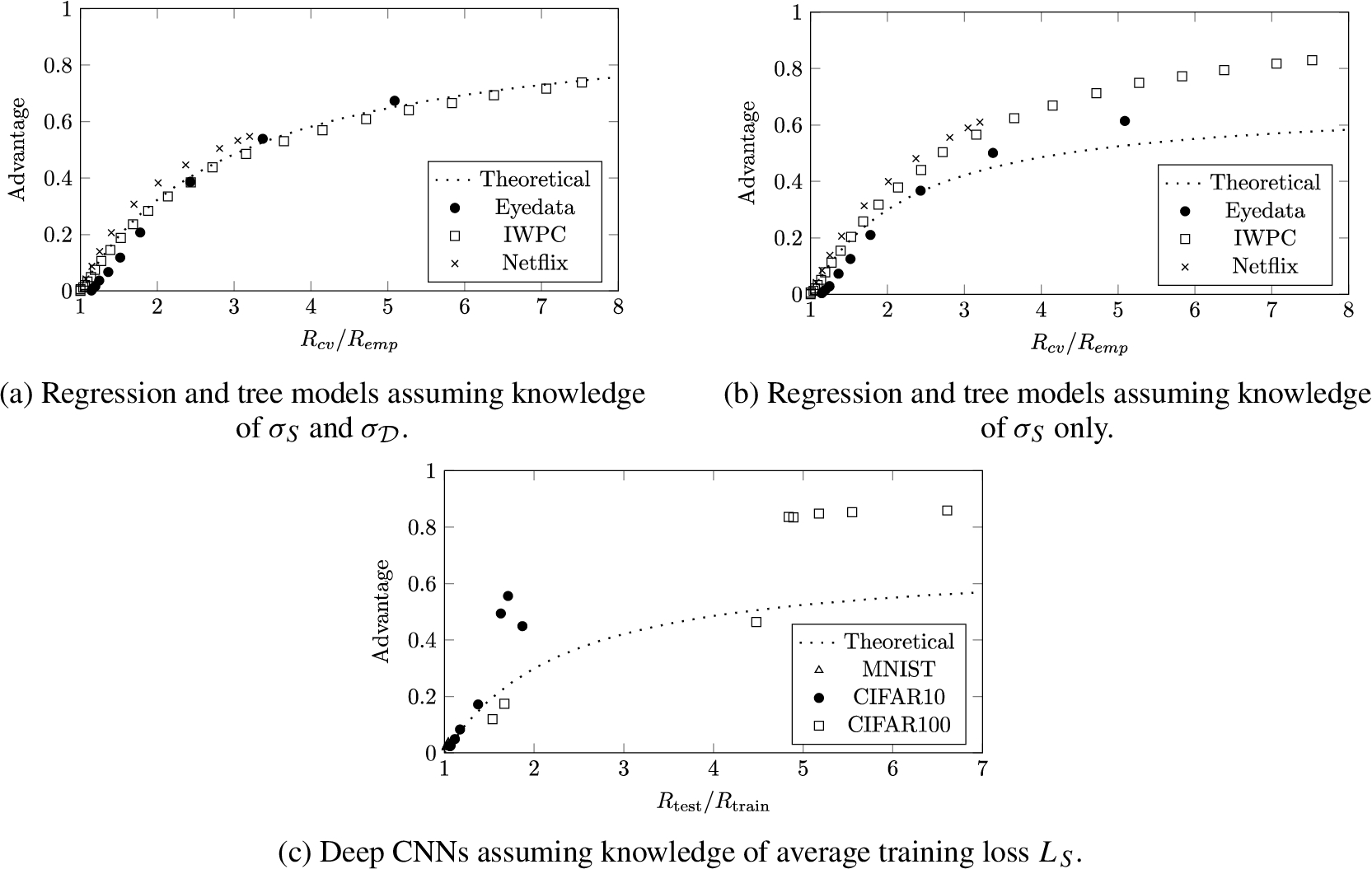
Fig. 3.
The training and test error distributions for an overfitted decision tree. The histograms are juxtaposed with what we would expect if the errors were normally distributed with standard deviation
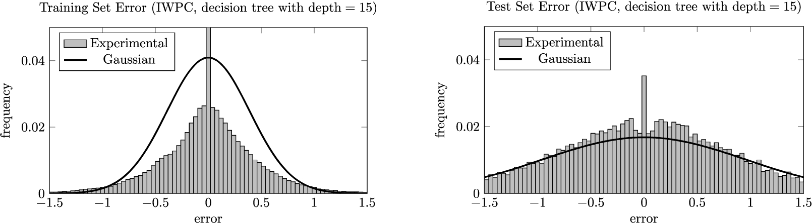
Fig. 4.
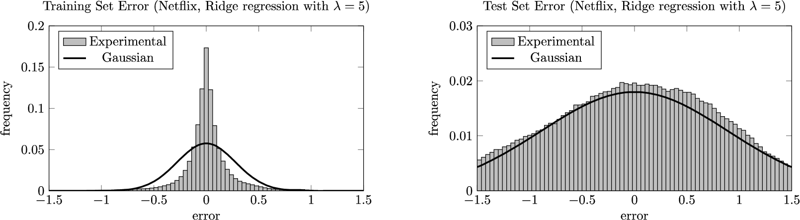
The training and test error distributions for an overfitted Ridge regression model. The histograms are juxtaposed with what we would expect if the errors were normally distributed with standard deviation
The results of the membership inference attacks on linear and tree models are plotted in Figs 2(a) and 2(b). The theoretical and experimental results appear to agree when the adversary knows both
The results of the threshold adversary on CNNs are given in Fig. 2(c). Although these models perform classification, the loss function used for training is categorical cross-entropy, which is non-negative, continuous, and unbounded. This suggests that the threshold adversary could potentially work in this setting as well. Specifically, the predictions made by these models can be compared against
Table 1
Comparison of our membership inference attack with that presented by Shokri et al. While our attack has slightly lower precision, it requires far less computational resources and background knowledge
| Our work | Shokri et al. [54] | |
| Attack complexity | Makes only one query to the model | Must train dozens of shadow models |
| Required knowledge | Average training loss | Ability to train shadow models, e.g., input distribution and type of model |
| Precision | 0.505 (MNIST) 0.694 (CIFAR-10) 0.874 (CIFAR-100) | 0.517 (MNIST) 0.72–0.74 (CIFAR-10) |
| Recall |
Now we compare our attack with that by Shokri et al. [54], which generates “shadow models” that are intended to mimic the behavior of
7.3.Attribute inference and reduction
Fig. 5.
Experimentally determined advantage for various membership and attribute adversaries.
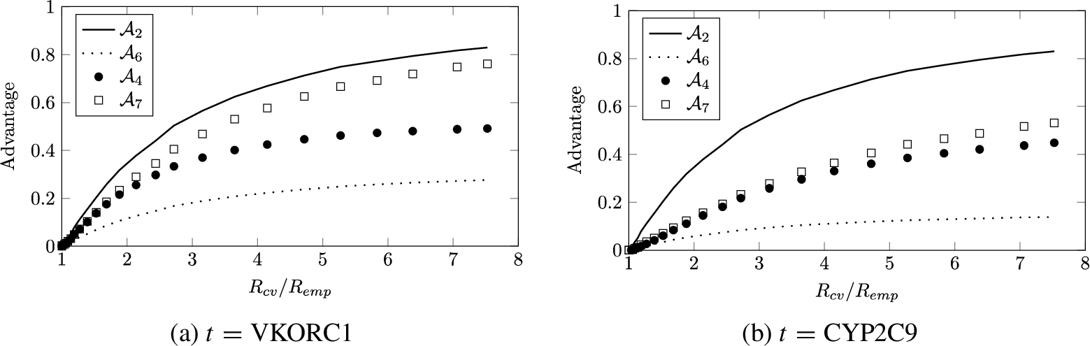
We now present the empirical attribute advantage of the general adversary (Adversary 4). Because this adversary uses the model inversion assumptions described at the beginning of Section 4.1, our evaluation is also in the setting of model inversion. For these experiments we used the IWPC and Netflix datasets described in Section 7.1. For
The circles in Fig. 5 show the result of inverting the VKORC1 and CYP2C9 attributes in the IWPC dataset. Although the attribute advantage is not as high as the membership advantage (solid line), the attribute adversary exhibits a sizable advantage that increases as the model overfits more and more. On the other hand, none of the attacks could effectively infer whether a user watched a certain movie in the Netflix dataset. In addition, we were unable to simultaneously control for both
Finally, we evaluate the performance of the multi-query reduction adversary (Adversary 7). As the squares in Fig. 5 show, with the IWPC data, making multiple queries to the membership oracle significantly increased the success rate compared to what we would expect from the naive uniform reduction adversary (Adversary 6, dotted line). Surprisingly, the reduction is also more effective than running the attribute inference attack directly. By contrast, with the Netflix data, the multi-query reduction adversary was often slightly worse than the naive uniform adversary although it still outperformed direct attribute inference.
7.4.Collusion in membership inference
We evaluate
Fig. 6.
Results of the colluding training algorithm (Algorithm 1) and the colluding membership adversary (Adversary 3) on CNNs trained on MNIST, CIFAR-10, and CIFAR-100. The size parameter was configured to take values
![Results of the colluding training algorithm (Algorithm 1) and the colluding membership adversary (Adversary 3) on CNNs trained on MNIST, CIFAR-10, and CIFAR-100. The size parameter was configured to take values s=2i for i∈[0,7]. Regardless of the models’ generalization performance, when the network is sufficiently large, the attack achieves high advantage (⩾0.98) without affecting predictive accuracy.](https://content.iospress.com:443/media/jcs/2020/28-1/jcs-28-1-jcs191362/jcs-28-jcs191362-g006.jpg)
The results of our experiment are shown in Figs 6(a) and 6(b). The data shows that on all three instances, the colluding parties achieve a high membership advantage without significantly affecting model performance. The accuracy of the subverted model was only 0.014 (MNIST), 0.047 (CIFAR-10), and 0.031 (CIFAR-100) less than that of the unsubverted model. The advantage rapidly increases with the model size around
Importantly, the results demonstrate that specific information about nearly all of the training data can be intentionally leaked through the behavior of a model that appears to generalize very well. In fact, looking at Fig. 6(b) shows that in these instances, there is no discernible relationship between generalization error and membership advantage. The three datasets exhibit vastly different generalization behavior, with the MNIST models achieving almost no generalization error (
7.5.Robustness
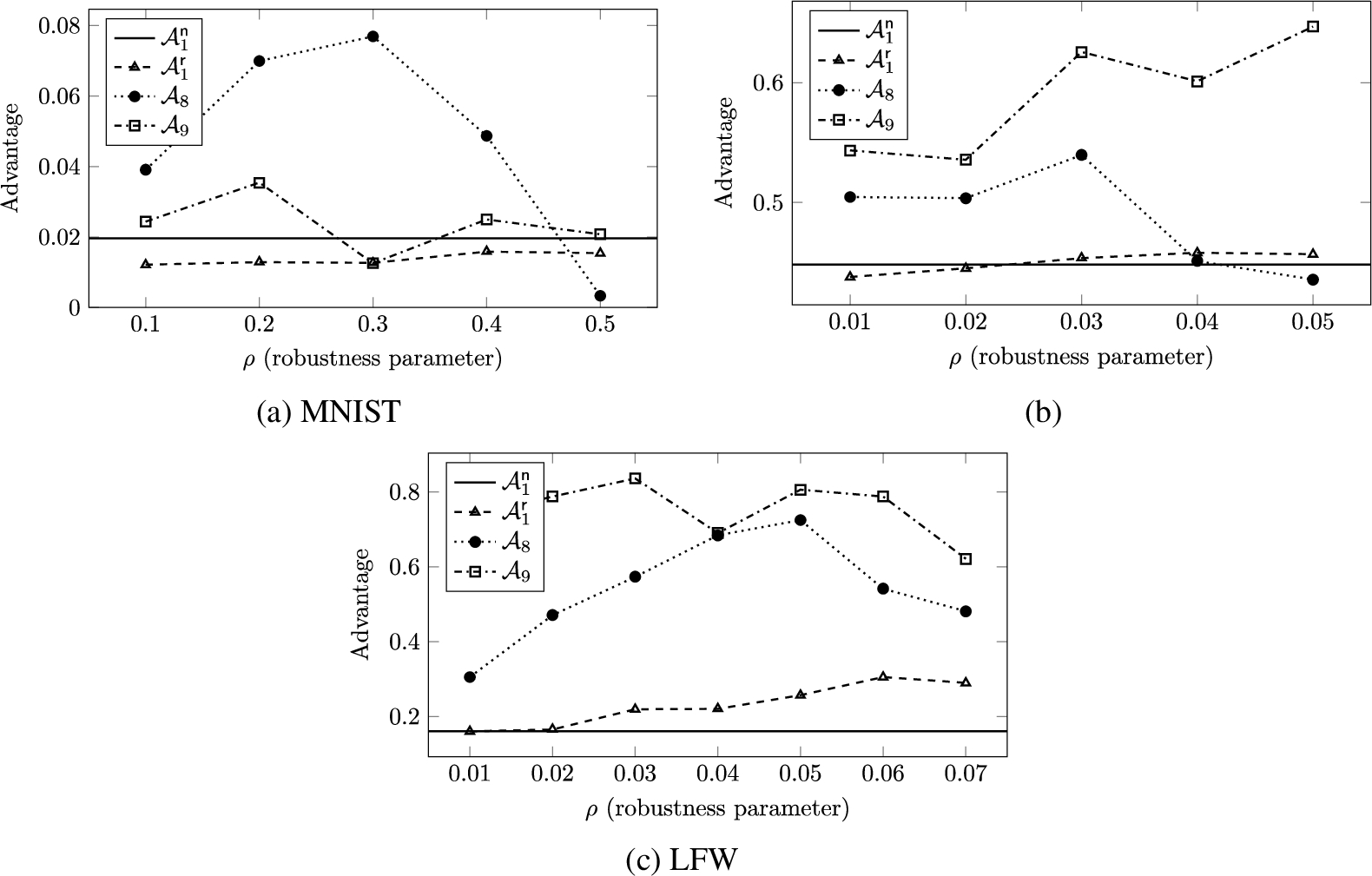
Fig. 7.
Experimentally determined membership advantage for various adversaries on robust classification models.
In this section, we evaluate the attacks against robust models. These attacks (Adversaries 8 and 9) use projected gradient descent to gain information about the robustness of a classifier around a given point, which is then used to infer whether the point is in the training set. Thus, these attacks differ from the other attacks presented in this article in that they are not fully black-box attacks. We compare the results to those of the simple bounded-loss membership adversary (Adversary 1), showing that in many cases robustness can leak membership information beyond that leaked by overfitting.
In Fig. 7, we plot the membership advantage on robust models with different values of the robustness parameter ρ. The inputs to these models, which are all images, had their pixel values scaled to be between 0 and 1, and the
However, under many other settings, the robust classification adversary outperformed the bounded-loss adversary on both non-robust (solid line) and robust (triangles) models. Recall from Theorem 2 that the bounded-loss adversary achieves an advantage equal to the generalization error for classification tasks where the 0–1 loss is used. When the robust model was able to classify the training points robustly with near-perfect accuracy, the robust loss on the test set was often greater than the standard loss on the test set. Thus, by leveraging the difference in the robust loss between the training and test sets, the robust classification adversary was able to achieve a larger advantage than the bounded-loss adversary, which uses the difference in the standard loss.
On the other hand, on the CIFAR-100 dataset the robust classification adversary was not significantly better, and was in some cases worse. This is because the model was unable to learn a robust decision boundary, meaning that the robust loss on the training set was greater than the standard loss on the training set. This difference offset the improvement over the bounded-loss adversary that was gained through the aforementioned difference between the robust and standard losses on the test set.
Finally, the results of the robust threshold adversary (Adversary 9) are plotted as squares in Fig. 7, showing that the adversary performed even better than the robust classification adversary on the CIFAR-10 and LFW datasets. Notably, in many LFW settings the advantage was around 0.8, which corresponds to correctly guessing membership in the training set 90% of the time. In addition, although the performance on CIFAR-10 is not as good as that of the shadow model attack by Shokri et al. [54], it is remarkable for two reasons: First, we only trained one shadow model per attack, whereas Shokri et al. evaluated their attacks with 10–100 shadow models. Second, unlike their attack model, which is a neural network that uses the full prediction vector output by the softmax layer, ours is a logistic regression model that takes in only three inputs (
8.Related work
This article is an extension of a prior conference publication [68], which identifies overfitting and malicious training algorithms as sources of privacy risk. In the current version, we additionally formalize and evaluate attacks against robust models, identifying robustness as another source of privacy risk. Other closely related prior work falls roughly into two categories: privacy in summary statistics, and privacy in machine learning applications. Throughout the article we discussed other, more distantly related work on machine learning, differential privacy, robustness, and other topics when it was contextually relevant.
8.1.Privacy and statistical summaries
There is extensive prior literature on privacy attacks on statistical summaries outside the context of machine learning. We refer the reader to a survey by De Capitani di Vimercati et al. [15] for a summary of the various definitions of privacy and the data protection techniques. Komarova et al. [34] looked into partial disclosure scenarios, where an adversary is given fixed statistical estimates from combined public and private sources and attempts to infer the sensitive feature of an individual referenced in those sources. A number of previous studies [21,27,28,50,55,62] have looked into membership attacks from statistics commonly published in genome-wide association studies (GWAS). Calandrino et al. [10] showed that temporal changes in recommendations given by collaborative filtering methods can reveal the inputs that caused those changes. Linear reconstruction attacks [16,20,32] attempt to infer partial inputs to linear statistics and were later extended to non-linear statistics [31]. While the goal of these attacks has commonalities with both membership inference and attribute inference, our results apply specifically to machine learning settings where generalization error and influence make our results relevant.
8.2.Privacy and machine learning
More recently, others have begun examining these attacks in the context of machine learning. Ateniese et al. [3] showed that the knowledge of the internal structure of Support Vector Machines and Hidden Markov Models leaks certain types of information about their training data, such as the language used in a speech dataset.
Dwork et al. [19] showed that a differentially private algorithm with a suitably chosen parameter generalizes well with high probability. Subsequent work showed that similar results are true under related notions of privacy. In particular, Bassily et al. [4] studied a notion of privacy called total variation stability and proved good generalization with respect to a bounded number of adaptively chosen low-sensitivity queries. Moreover, for data drawn from Gibbs distributions, Wang et al. [64] showed that on-average KL privacy is equivalent to generalization error as defined in this article. While these results give evidence for the relationship between privacy and overfitting, we construct an attacker that directly leverages overfitting to gain advantage commensurate with the extent of the overfitting.
8.2.1.Membership inference
Shokri et al. [54] developed a membership inference attack and applied it to popular machine-learning-as-a-service APIs. Their attacks are based on “shadow models” that approximate the behavior of the model under attack. The shadow models are used to build another machine learning model called the “attack model”, which is trained to distinguish points in the training data from other points based on the output they induce on the original model under attack. As we discussed in Section 7.2, our simple threshold adversary comes surprisingly close to the accuracy of their attack, especially given the differences in complexity and requisite adversarial assumptions between the attacks.
Because the attack proposed by Shokri et al. itself relies on machine learning to find a function that separates training and non-training points, it is not immediately clear why the attack works, but the authors hypothesize that it is related to overfitting and the “diversity” of the training data. They graph the generalization error against the precision of their attack and find some evidence of a relationship, but they also find that the relationship is not perfect and conclude that model structure must also be relevant. The results presented in this article make the connection to overfitting precise in many settings, and the colluding training algorithm we give in Section 7.4 demonstrates exactly how model structure can be exploited to create a membership inference vulnerability.
Li et al. [39] explored membership inference, distinguishing between “positive” and “negative” membership privacy. They show how this framework defines a family of related privacy definitions that are parametrized on distributions of the adversary’s prior knowledge, and they find that a number of previous definitions can be instantiated in this way.
8.2.2.Attribute inference
Practical model inversion attacks have been studied in the context of linear regression [23,67], decision trees [22], and neural networks [22]. Our results apply to these attacks when they are applied to data that matches the distributional assumptions made in our analysis. An important distinction between the way inversion attacks were considered in prior work and how we treat them here is the notion of advantage. Prior work on these attacks defined advantage as the difference between the attacker’s predictive accuracy given the model and the best accuracy that could be achieved without the model. Although some prior work [22,23] empirically measured this advantage on both training and test datasets, this definition does not allow a formal characterization of how exposed the training data specifically is to privacy risk. In Section 4, we define attribute advantage precisely to capture the risk to the training data by measuring the difference in the attacker’s accuracy on training and test data: the advantage is zero when the attack is as powerful on the general population as on the training data and is maximized when the attack works only on the training data.
Wu et al. [66] formalized model inversion for a simplified class of models that consist of Boolean functions and explored the initial connections between influence and advantage. However, as in other prior work on model inversion, the type of advantage that they consider says nothing about what the model specifically leaks about its training data. Drawing on their observation that influence is relevant to privacy risk in general, we illustrate its effect on the notion of advantage defined in this article and show how it interacts with generalization error.
8.2.3.Robustness
Many researchers [49,61,70] recently noted that robustness tends to lower the standard (non-robust) accuracy of the robust model. This tends to increase the standard generalization error, and as we prove that generalization error necessarily leads to privacy risk in many settings, these results support the notion that robustness is at odds with privacy. However, our result goes further, showing a membership adversary can leverage the robust generalization error, which is often even larger than the standard generalization error. Schmidt et al. [52] argued that robust learning has a higher sample complexity than standard learning. Thus, a larger training set may be a possible defense to membership inference attacks based on the robust generalization error.
In a concurrent work, Song et al. [58] evaluate several different attacks that seek to extract membership information from robust models, showing that robustness can make a model more vulnerable to membership inference. Although the attacks that we present within our formal framework are similar to theirs, our experimental setup has a few major differences. First, their simple attack uses the confidence of the robust model’s prediction, whereas our simple attack only considers its correctness. Second, their shadow model attack uses several perturbations of the given point, each generated with a different target class, whereas our shadow model attack only considers the distances to the nearest decision boundary. Despite these differences, our results agree in substance with those of Song et al., providing additional evidence that robustness can lead to increased privacy risk.
9.Conclusion and future directions
We introduced new formal definitions of advantage for membership and attribute inference attacks. Using these definitions, we analyzed attacks under various assumptions on learning algorithms and model properties, and we showed that these two attacks are closely related through reductions in both directions. Both theoretical and experimental results confirm that models become more vulnerable to both types of attacks as they overfit more. Interestingly, our analysis also shows that overfitting is not the only factor that can lead to privacy risk: The results in Section 4.1 demonstrate that the influence of the target attribute on a model’s output plays a key role in attribute inference, and Theorem 4 in Section 3.4 shows that even stable learning algorithms, which provably do not overfit, can leak precise membership information. In addition, our experiments in Section 7.5 point to robustness as another source of membership advantage, suggesting that it may be difficult to defend against both privacy and integrity attacks simultaneously. We thus identify as future work the training of robust models without leaking membership information.
Our formalization and analysis also open other interesting directions for future work. The membership attack in Theorem 4 is based on a colluding pair of adversary and learning algorithm,
Our results in Section 3.1 give bounds on membership advantage when certain conditions are met. These bounds apply to adversaries who may target specific individuals, bringing arbitrary background knowledge of their targets to help determine their membership status. Some types of realistic adversaries may be motivated by concerns that incentivize learning a limited set of facts about as many individuals in the training data as possible rather than obtaining unique background knowledge about specific individuals. Characterizing these “stable adversaries” is an interesting direction that may lead to tighter bounds on advantage or relaxed conditions on the learning algorithm.
Acknowledgments
The authors would like to thank the anonymous reviewers at the IEEE Computer Security Foundations Symposium (CSF) and the Journal of Computer Security for their thoughtful feedback. This material is based upon work supported by the National Science Foundation (NSF) under Grant No. CNS-1704845. Somesh Jha was partially supported by NSF Grants CCF-1836978, CNS-1804648, and CCF-1652140; Air Force Grant FA9550-18-1-0166; and Army Research Office Grant W911NF-17-1-0405.
References
[1] | M. Abadi, A. Agarwal, P. Barham, E. Brevdo, Z. Chen, C. Citro, G.S. Corrado, A. Davis, J. Dean, M. Devin, S. Ghemawat, I. Goodfellow, A. Harp, G. Irving, M. Isard, Y. Jia, R. Jozefowicz, L. Kaiser, M. Kudlur, J. Levenberg, D. Mané, R. Monga, S. Moore, D. Murray, C. Olah, M. Schuster, J. Shlens, B. Steiner, I. Sutskever, K. Talwar, P. Tucker, V. Vanhoucke, V. Vasudevan, F. Viégas, O. Vinyals, P. Warden, M. Wattenberg, M. Wicke, Y. Yu and X. Zheng, TensorFlow: Large-scale machine learning on heterogeneous systems, 2015. |
[2] | G. Ateniese, B. Magri and D. Venturi, Subversion-resilient signature schemes, in: ACM Conference on Computer and Communications Security, (2015) , pp. 364–375. |
[3] | G. Ateniese, L.V. Mancini, A. Spognardi, A. Villani, D. Vitali and G. Felici, Hacking smart machines with smarter ones: How to extract meaningful data from machine learning classifiers, International Journal of Security and Networks 10: (3) ((2015) ), 137–150. doi:10.1504/IJSN.2015.071829. |
[4] | R. Bassily, K. Nissim, A. Smith, T. Steinke, U. Stemmer and J. Ullman, Algorithmic stability for adaptive data analysis, in: ACM Symposium on Theory of Computing, (2016) , pp. 1046–1059. |
[5] | R. Bassily, A. Smith and A. Thakurta, Private empirical risk minimization: Efficient algorithms and tight error bounds, in: IEEE Symposium on Foundations of Computer Science, (2014) . |
[6] | M. Bellare, J. Jaeger and D. Kane, Mass-surveillance without the state: Strongly undetectable algorithm-substitution attacks, in: ACM Conference on Computer and Communications Security, (2015) , pp. 1431–1440. |
[7] | M. Bellare, K.G. Paterson and P. Rogaway, Security of symmetric encryption against mass surveillance, in: Advances in Cryptology – CRYPTO, (2014) , pp. 1–19. |
[8] | O. Bousquet and A. Elisseeff, Stability and generalization, Journal of Machine Learning Research 2: ((2002) ), 499–526. |
[9] | J. Brickell and V. Shmatikov, The cost of privacy: Destruction of data-mining utility in anonymized data publishing, in: ACM SIGKDD Conference on Knowledge Discovery and Data Mining, (2008) , pp. 70–78. |
[10] | J.A. Calandrino, A. Kilzer, A. Narayanan, E.W. Felten and V. Shmatikov, “you might also like:” privacy risks of collaborative filtering, in: IEEE Symposium on Security and Privacy (Oakland), (2011) . |
[11] | K. Chaudhuri, C. Monteleoni and A.D. Sarwate, Differentially private empirical risk minimization, Journal of Machine Learning Research (2011). |
[12] | F. Chollet et al., Keras, 2015. |
[13] | J. Cohen, E. Rosenfeld and Z. Kolter, Certified adversarial robustness via randomized smoothing, in: Proceedings of the 36th International Conference on Machine Learning, K. Chaudhuri and R. Salakhutdinov, eds, Proceedings of Machine Learning Research, Vol. 97: , (2019) , pp. 1310–1320. |
[14] | G. Cormode, Personal privacy vs population privacy: Learning to attack anonymization, in: ACM SIGKDD Conference on Knowledge Discovery and Data Mining, (2011) , pp. 1253–1261. |
[15] | S. De Capitani di Vimercati, S. Foresti, G. Livraga and P. Samarati, Data privacy: Definitions and techniques, International Journal of Uncertainty, Fuzziness and Knowledge-Based Systems 20: (6) ((2012) ), 793–817. doi:10.1142/S0218488512400247. |
[16] | I. Dinur and K. Nissim, Revealing information while preserving privacy, in: ACM SIGMOD-SIGACT-SIGART Symposium on Principles of Database Systems, (2003) , pp. 202–210. |
[17] | C. Dwork, Differential privacy, in: International Colloquium on Automata, Languages and Programming, (2006) , pp. 1–12. |
[18] | C. Dwork, V. Feldman, M. Hardt, T. Pitassi, O. Reingold and A. Roth, Generalization in adaptive data analysis and holdout reuse, in: Neural Information Processing Systems, (2015) , pp. 2350–2358. |
[19] | C. Dwork, V. Feldman, M. Hardt, T. Pitassi, O. Reingold and A.L. Roth, Preserving statistical validity in adaptive data analysis, in: ACM Symposium on Theory of Computing, (2015) , pp. 117–126. |
[20] | C. Dwork, F. McSherry and K. Talwar, The price of privacy and the limits of LP decoding, in: ACM Symposium on Theory of Computing, (2007) , pp. 85–94. |
[21] | K. El Emam, E. Jonker, L. Arbuckle and B. Malin, A systematic review of re-identification attacks on health data, PLOS ONE 6: (12) ((2011) ), 1–12. |
[22] | M. Fredrikson, S. Jha and T. Ristenpart, Model inversion attacks that exploit confidence information and basic countermeasures, in: ACM Conference on Computer and Communications Security (CCS), (2015) . |
[23] | M. Fredrikson, E. Lantz, S. Jha, S. Lin, D. Page and T. Ristenpart, Privacy in pharmacogenetics: An end-to-end case study of personalized warfarin dosing, in: USENIX Security Symposium, (2014) , pp. 17–32. |
[24] | I. Giacomelli, R.F. Olimid and S. Ranellucci, Security of linear secret-sharing schemes against mass surveillance, in: Cryptology and Network Security – CANS, (2015) , pp. 43–58. doi:10.1007/978-3-319-26823-1_4. |
[25] | I. Goodfellow, Y. Bengio and A. Courville, Deep Learning, MIT Press, (2016) , http://www.deeplearningbook.org. |
[26] | I.J. Goodfellow, J. Shlens and C. Szegedy, Explaining and harnessing adversarial examples, in: International Conference on Learning Representations, (2015) . |
[27] | M. Gymrek, A.L. McGuire, D. Golan, E. Halperin and Y. Erlich, Identifying personal genomes by surname inference, Science 339: (6117) ((2013) ), 321–324. doi:10.1126/science.1229566. |
[28] | N. Homer, S. Szelinger, M. Redman, D. Duggan, W. Tembe, J. Muehling, J.V. Pearson, D.A. Stephan, S.F. Nelson and D.W. Craig, Resolving individuals contributing trace amounts of DNA to highly complex mixtures using high-density SNP genotyping microarrays, PLoS Genetics 4: (8) ((2008) ), e1000167. doi:10.1371/journal.pgen.1000167. |
[29] | G.B. Huang, M. Ramesh, T. Berg and E. Learned-Miller, Labeled faces in the wild: A database for studying face recognition in unconstrained environments, Technical Report, 07-49, University of Massachusetts, Amherst, 2007. |
[30] | International Warfarin Pharmacogenetics Consortium, Estimation of the warfarin dose with clinical and pharmacogenetic data, New England Journal of Medicine 360: (8) ((2009) ), 753–764. doi:10.1056/NEJMoa0809329. |
[31] | S.P. Kasiviswanathan, M. Rudelson and A. Smith, The power of linear reconstruction attacks, in: ACM-SIAM Symposium on Discrete Algorithms, (2013) , pp. 1415–1433. doi:10.1137/1.9781611973105.102. |
[32] | S.P. Kasiviswanathan, M. Rudelson, A. Smith and J. Ullman, The price of privately releasing contingency tables and the spectra of random matrices with correlated rows, in: ACM Symposium on Theory of Computing, (2010) , pp. 775–784. |
[33] | D.P. Kingma and J. Ba, Adam: A method for stochastic optimization, in: International Conference for Learning Representations (ICLR), (2015) . |
[34] | T. Komarova, D. Nekipelov and E. Yakovlev, Estimation of treatment effects from combined data: Identification versus data security, in: Economic Analysis of the Digital Economy, (2015) , pp. 279–308. doi:10.7208/chicago/9780226206981.003.0010. |
[35] | P. Krähenbühl, C. Doersch, J. Donahue and T. Darrell, Data-dependent initializations of convolutional neural networks, arXiv preprint arXiv:1511.06856 (2015). |
[36] | A. Krizhevsky and G. Hinton, Learning multiple layers of features from tiny images (2009). |
[37] | Y. LeCun, C. Cortes and C. Burges, The MNIST database of handwritten digits, 1998. |
[38] | J. Lei, Differentially private m-estimators, in: Neural Information Processing Systems, (2011) , pp. 361–369. |
[39] | N. Li, W. Qardaji, D. Su, Y. Wu and W. Yang, Membership privacy: A unifying framework for privacy definitions, in: ACM SIGSAC Conference on Computer and Communications Security, (2013) , pp. 889–900. |
[40] | A. Mądry, A. Makelov, L. Schmidt, D. Tsipras and A. Vladu, Towards deep learning models resistant to adversarial attacks, in: International Conference on Learning Representations, (2018) . |
[41] | K.P. Murphy, Machine Learning: A Probabilistic Perspective, The MIT Press, (2012) . |
[42] | Netflix, Netflix Prize, 2006. |
[43] | B. Neuberg, Personal Photos Model, GitHub, 2017. |
[44] | R. O’Donnell, Analysis of Boolean Functions, Cambridge University Press, (2014) . doi:10.1017/CBO9781139814782. |
[45] | N. Papernot, F. Faghri, N. Carlini, I. Goodfellow, R. Feinman, A. Kurakin, C. Xie, Y. Sharma, T. Brown, A. Roy, A. Matyasko, V. Behzadan, K. Hambardzumyan, Z. Zhang, Y.-L. Juang, Z. Li, R. Sheatsley, A. Garg, J. Uesato, W. Gierke, Y. Dong, D. Berthelot, P. Hendricks, J. Rauber and R. Long, Technical report on the CleverHans v2.1.0 adversarial examples library, arXiv preprint arXiv:1610.00768 (2018). |
[46] | N. Papernot, P. McDaniel, I. Goodfellow, S. Jha, Z.B. Celik and A. Swami, Practical black-box attacks against machine learning, in: Proceedings of the 2017 ACM on Asia Conference on Computer and Communications Security, (2017) . |
[47] | N. Papernot, P. McDaniel, S. Jha, M. Fredrikson, Z.B. Celik and A. Swami, The limitations of deep learning in adversarial settings, in: IEEE European Symposium on Security and Privacy, (2016) , pp. 372–387. |
[48] | F. Pedregosa, G. Varoquaux, A. Gramfort, V. Michel, B. Thirion, O. Grisel, M. Blondel, P. Prettenhofer, R. Weiss, V. Dubourg, J. Vanderplas, A. Passos, D. Cournapeau, M. Brucher, M. Perrot and E. Duchesnay, Scikit-learn: Machine learning in python, Journal of Machine Learning Research 12: ((2011) ), 2825–2830. |
[49] | A. Raghunathan, S.M. Xie, F. Yang, J.C. Duchi and P. Liang, Adversarial training can hurt generalization, arXiv preprint arXiv:1906.06032 (2019). |
[50] | S. Sankararaman, G. Obozinski, M.I. Jordan and E. Halperin, Genomic privacy and limits of individual detection in a pool, Nature Genetics 41: (9) ((2009) ), 965–967. doi:10.1038/ng.436. |
[51] | T.E. Scheetz, K.-Y.A. Kim, R.E. Swiderski, A.R. Philp, T.A. Braun, K.L. Knudtson, A.M. Dorrance, G.F. DiBona, J. Huang, T.L. Casavant, V.C. Sheffield and E.M. Stone, Regulation of gene expression in the mammalian eye and its relevance to eye disease, Proceedings of the National Academy of Sciences 103: (39) ((2006) ), 14429–14434. doi:10.1073/pnas.0602562103. |
[52] | L. Schmidt, S. Santurkar, D. Tsipras, K. Talwar and A. Madry, Adversarially robust generalization requires more data, in: Advances in Neural Information Processing Systems, (2018) , pp. 5014–5026. |
[53] | S. Shalev-Shwartz, O. Shamir, N. Srebro and K. Sridharan, Learnability, stability and uniform convergence, Journal of Machine Learning Research 11: ((2010) ). |
[54] | R. Shokri, M. Stronati, C. Song and V. Shmatikov, Membership inference attacks against machine learning models, in: IEEE Symposium on Security and Privacy (Oakland), (2017) , pp. 3–18. |
[55] | S.S. Shringarpure and C.D. Bustamante, Privacy risks from genomic data-sharing beacons, The American Journal of Human Genetics 97: (5) ((2015) ), 631–646. doi:10.1016/j.ajhg.2015.09.010. |
[56] | K. Simonyan and A. Zisserman, Very deep convolutional networks for large-scale image recognition, arXiv preprint arXiv:1409.1556 (2014). |
[57] | C. Song, T. Ristenpart and V. Shmatikov, Machine learning models that remember too much, in: ACM Conference on Computer and Communications Security, (2017) , pp. 587–601. |
[58] | L. Song, R. Shokri and P. Mittal, Privacy risks of securing machine learning models against adversarial examples, arXiv preprint arXiv:1905.10291 (2019). |
[59] | C. Szegedy, W. Zaremba, I. Sutskever, J. Bruna, D. Erhan, I. Goodfellow and R. Fergus, Intriguing properties of neural networks, in: International Conference on Learning Representations, (2014) . http://arxiv.org/abs/1312.6199. |
[60] | A.G. Thakurta and A. Smith, Differentially private feature selection via stability arguments, and the robustness of the lasso, in: Conference on Learning Theory, Vol. 30: , (2013) , pp. 819–850. |
[61] | D. Tsipras, S. Santurkar, L. Engstrom, A. Turner and A. Madry, Robustness may be at odds with accuracy, in: International Conference on Learning Representations, (2019) . |
[62] | R. Wang, Y.F. Li, X. Wang, H. Tang and X. Zhou, Learning your identity and disease from research papers: Information leaks in genome wide association studies, in: ACM Conference on Computer and Communications Security, (2009) , pp. 534–544. |
[63] | Y.-X. Wang, J. Lei and S.E. Fienberg, Learning with differential privacy: Stability, learnability and the sufficiency and necessity of ERM principle, Journal of Machine Learning Research 17: (183) ((2016) ), 1–40. |
[64] | Y.-X. Wang, J. Lei and S.E. Fienberg, On-average KL-privacy and its equivalence to generalization for max-entropy mechanisms, in: Privacy in Statistical Databases, (2016) , pp. 121–134. doi:10.1007/978-3-319-45381-1_10. |
[65] | E. Wong and Z. Kolter, Provable defenses against adversarial examples via the convex outer adversarial polytope, in: International Conference on Machine Learning, (2018) , pp. 5283–5292. |
[66] | X. Wu, M. Fredrikson, S. Jha and J.F. Naughton, A methodology for formalizing model-inversion attacks, in: IEEE Computer Security Foundations Symposium (CSF), (2016) . |
[67] | X. Wu, M. Fredrikson, W. Wu, S. Jha and J.F. Naughton, Revisiting Differentially private regression: Lessons from learning theory and their consequences, arXiv preprint arXiv:1512.06388 (2015). |
[68] | S. Yeom, I. Giacomelli, M. Fredrikson and S. Jha, Privacy risk in machine learning: Analyzing the connection to overfitting, in: IEEE Computer Security Foundations Symposium (CSF), (2018) , pp. 268–282. |
[69] | C. Zhang, S. Bengio, M. Hardt, B. Recht and O. Vinyals, Understanding deep learning requires rethinking generalization, arXiv preprint arXiv:1611.03530 (2016). |
[70] | H. Zhang, Y. Yu, J. Jiao, E. Xing, L. El Ghaoui and M. Jordan, Theoretically principled trade-off between robustness and accuracy, in: International Conference on Machine Learning, (2019) , pp. 7472–7482. |
[71] | J. Zhang, Z. Zhang, X. Xiao, Y. Yang and M. Winslett, Functional mechanism: Regression analysis under differential privacy, Proceedings of the VLDB Endowment 5: (11) ((2012) ), 1364–1375. doi:10.14778/2350229.2350253. |


